Aug 3, 2005 - Scheffé). He also constructed conservative GCIs for all pairwise ..... Lehmann-Scheffé theorem: Suppose t is a complete and sufficient vector for.
DISSERTATION
APPLICATIONS OF GENERALIZED INFERENCE
Submitted by Amany Hassan Abdel-Karim Department of Statistics
In partial fulfillment of the requirements For the Degree of Doctor of Philosophy Colorado State University Fort Collins, Colorado Fall 2005
COLORADO STATE UNIVERSITY
August 3, 2005 WE HEREBY RECOMMEND THAT THE DISSERTATION PREPARED UNDER OUR SUPERVISION BY AMANY HASSAN ABDEL-KARIM ENTITLED APPLICATIONS OF GENERALIZED INFERENCE BE ACCEPTED AS FULFILLING IN PART REQUIREMENTS FOR THE DEGREE OF DOCTOR OF PHILOSOPHY.
Committee on Graduate Work
Committee Member Committee Member Committee Member Hariharan Iyer (Adviser) Jan Hannig (Co-Adviser) F. Jay Breidt (Department Head)
ii
ABSTRACT OF DISSERTATION APPLICATIONS OF GENERALIZED INFERENCE There are many statistical inference problems in mixed linear models for which exact solutions are not available. In these cases, standard statistical software packages such as SAS and S-PLUS either use asymptotic procedures or methods based on the Satterthwaite-type approximations. In this dissertation, it is shown that generalized inference (generalized pivotal quantity, generalized confidence interval, generalized test variable and generalized P -value) may be used as an alternative to asymptotic approximations or other small sample approximations. After presenting the definitions pertaining to generalized inference, we show how to extend the concept of generalized confidence intervals to generalized simultaneous confidence intervals. We also show how to extend generalized tests of hypotheses to multiparameter problems. Specifically, the following problems were addressed. 1. All pairwise comparisons of cell means in unbalanced heterogeneous one-way ANOVA (Extended Tukey) 2. Pairwise comparisons of treatment means to a control mean in unbalanced heterogeneous one-way ANOVA (Extended Dunnett) 3. All cell means in balanced two-factor crossed mixed linear model. 4. All pairwise comparisons of cell means in balanced three-factor nested factorial mixed linear model. Other applications considered in this dissertation include the use of generalized confidence intervals to choose between two non-nested linear models when the response and the predictors have jointly a multivariate normal distribution. Generalized tests were developed for the following problems. iii
1. Testing the equality of the cell means in unbalanced heterogeneous one-way ANOVA 2. Testing the equality of the cell means in balanced three-factor crossed mixed linear model with interactions. Simulation studies were used to estimate the error rates for each problem considered. Comparisons to other existing procedures were carried out when appropriate.
iv
ACKNOWLEDGEMENTS
My sincerest thanks to my supervisor, Dr. Hariharan Iyer for his continuous support and encouragement throughout the completion of my program. His help exceeded my expectation and conversations with him were always able to turn moments of desperation into moments of inspiration with new insights and goals to pursue. His valuable advice enormously helped me to finalize this dissertation. I am also grateful to my co-supervisor, Dr. Jan Hannig for his help and support. I am very grateful to Dr. David Bowden, Dr. Phillip Chapman and Dr. Eugene Allgower for agreeing to serve in my committee. Their constructive criticism and valuable advice added great values to this work. I am indebted the Egyptian Government and University of Tanta for providing me the scholarship for studying abroad. This gave me the chance to learn a lot not only in Statistics, but also in all aspects of life. I am so grateful to all members of the Department of Statistics, Colorado State University for providing me the opportunity and facilities throughout the work on my program. Their help has been essential to me and their co-operation is highly appreciated. I would like to thank my husband, Hatem, and sons, Ayman and Akram for their patience and sacrifices to get my degree completed. My greatest gratitude to my parents for their support by being good parents to me throughout my life.
v
CONTENTS
1 Introduction
1
2 Generalized Inference Definitions and Notations 6 2.1 Basic Definitions . . . . . . . . . . . . . . . . . . . . . . . . . . . . . 6 2.2 Generalized Inference . . . . . . . . . . . . . . . . . . . . . . . . . . . 7 2.3 Iyer and Patterson Recipe (2002) . . . . . . . . . . . . . . . . . . . . 10 3 Key Results from Linear Models and Mathematical Statistics 3.1 Matrix Results . . . . . . . . . . . . . . . . . . . . . . . . . . . . . . 3.1.1 Kronecker Products of Matrices . . . . . . . . . . . . . . . . . 3.1.2 Some Matrix Identities . . . . . . . . . . . . . . . . . . . . . . 3.2 Basic Results about Sufficiency, Completeness and Uniformly Minimum Variance Unbiased Estimators . . . . . . . . . . . . . . . . . . . 3.2.1 Complete and Sufficient Statistics in the Exponential Family . 3.2.2 Uniformly Minimum Variance Unbiased Estimator (UMVUE) 3.3 Results about Linear and Quadratic Forms . . . . . . . . . . . . . . . 3.4 A Summary of Tukey and Dunnett Procedures . . . . . . . . . . . . . 3.4.1 Tukey’s Simultaneous CIs . . . . . . . . . . . . . . . . . . . . 3.4.2 Dunnett’s CIs for Comparing all Means to a Control . . . . . 3.5 Balanced Mixed Linear Models . . . . . . . . . . . . . . . . . . . . . 3.6 Results about the Multivariate Normal Distribution . . . . . . . . . .
12 12 12 13
4 Simultaneous GCIs in One-way Classification Model 4.1 A Review for Multiple Comparisons of the Means in One-way Classification Model . . . . . . . . . . . . . . . . . . . . . . . . . . . . . 4.2 Extension of the Tukey Method for Heterogeneous, Unbalanced OneWay ANOVA Using GCIs . . . . . . . . . . . . . . . . . . . . . . . 4.3 Simulation Study . . . . . . . . . . . . . . . . . . . . . . . . . . . . 4.3.1 Simulation Details . . . . . . . . . . . . . . . . . . . . . . . 4.3.2 Discussion of Simulation Results . . . . . . . . . . . . . . . . 4.3.3 Comparison of Simultaneous GCIs with Dunnett (1980) Simultaneous CIs . . . . . . . . . . . . . . . . . . . . . . . . . 4.4 Example . . . . . . . . . . . . . . . . . . . . . . . . . . . . . . . . . 4.5 Extended Dunnett Method for Heterogeneous Unbalanced One-Way ANOVA . . . . . . . . . . . . . . . . . . . . . . . . . . . . . . . . .
24
vi
14 14 15 16 17 18 18 19 22
. 24 . . . .
28 30 31 32
. 34 . 34 . 35
4.6 Simulation Study . . . . . . . . . . . . . 4.6.1 Simulation Details . . . . . . . . 4.6.2 Discussion of Simulation Results . 4.7 Example . . . . . . . . . . . . . . . . . .
. . . .
. . . .
. . . .
. . . .
. . . .
. . . .
. . . .
. . . .
. . . .
. . . .
. . . .
. . . .
. . . .
. . . .
. . . .
. . . .
5 Applications of Generalized Inference in Balanced Mixed Linear Models 5.1 Review of Literature . . . . . . . . . . . . . . . . . . . . . . . . . . . 5.2 Simultaneous GCIs for all Means in Balanced Two-factor Crossed Mixed Linear Model with Interaction . . . . . . . . . . . . . . . . . . 5.3 Simulation Study . . . . . . . . . . . . . . . . . . . . . . . . . . . . . 5.3.1 Simulation Details . . . . . . . . . . . . . . . . . . . . . . . . 5.3.2 Discussion of Simulation Results . . . . . . . . . . . . . . . . . 5.4 Example . . . . . . . . . . . . . . . . . . . . . . . . . . . . . . . . . . 5.5 Simultaneous GCIs for all Pairwise Differences in Three-factor Nested-factorial Model . . . . . . . . . . . . . . . . . . . . . . . . . . 5.6 Simulation Study . . . . . . . . . . . . . . . . . . . . . . . . . . . . . 5.6.1 Simulation Details . . . . . . . . . . . . . . . . . . . . . . . . 5.6.2 Discussion of Simulation Results . . . . . . . . . . . . . . . . . 5.6.3 Comparison of GCIs with Intervals Obtained from SAS for all Pairwise Differences μij − μrs . . . . . . . . . . . . . . . . . . 5.7 Example . . . . . . . . . . . . . . . . . . . . . . . . . . . . . . . . . . 5.8 Appendix . . . . . . . . . . . . . . . . . . . . . . . . . . . . . . . . . 6 Using GCIs to Compare Non-nested Linear Models 6.1 Review of Literature . . . . . . . . . . . . . . . . . . . . . . . . . . 6.2 GCIs Method to Compare Non-Nested Subsets of Predictors . . . . 6.3 Simulation Study . . . . . . . . . . . . . . . . . . . . . . . . . . . . 6.3.1 Simulation Details . . . . . . . . . . . . . . . . . . . . . . . 6.3.2 Discussion of Simulation Results . . . . . . . . . . . . . . . . 6.3.3 Comparison of Results of GCIs with Ahlbrandt (1988) . . . 6.4 Example . . . . . . . . . . . . . . . . . . . . . . . . . . . . . . . . . 6.5 A Small Simulation Study to Assess the Performance of GCIs When the Number of Predictors is Large . . . . . . . . . . . . . . . . . . . 6.6 Appendix . . . . . . . . . . . . . . . . . . . . . . . . . . . . . . . . 7 Generalized Test Variables and Generalized Hypotheses Tests 7.1 Review of Literature . . . . . . . . . . . . . . . . . . . . . . . . . . 7.2 A General Approach for Constructing Generalized Tests . . . . . . 7.2.1 Testing Equality of Cell-Means in Unbalanced Heterogeneous One-Way ANOVA . . . . . . . . . . . . . . . . . . . . . . . 7.3 Simulation Study . . . . . . . . . . . . . . . . . . . . . . . . . . . . 7.3.1 Simulation Details . . . . . . . . . . . . . . . . . . . . . . . 7.3.2 Discussion of the Simulation Results . . . . . . . . . . . . . vii
. . . . . . .
37 37 38 40 41 41 43 47 48 50 50 62 66 67 69 69 75 83 86 86 92 94 94 96 97 97
. 98 . 100 101 . 101 . 104 . . . .
105 108 108 110
7.4 Example . . . . . . . . . . . . . . . . . . . . . . . . . . . . . . . . . 7.5 Test of Equality of Cell-Means in the Balanced Three-factor Crossed Mixed Linear Model with Interactions . . . . . . . . . . . . . . . . . 7.6 Simulation Study . . . . . . . . . . . . . . . . . . . . . . . . . . . . 7.6.1 Simulation Details . . . . . . . . . . . . . . . . . . . . . . . 7.6.2 Discussion of the Simulation Results . . . . . . . . . . . . . 7.6.3 Comparison of the Simulation Results for Testing μ1 = · · · = μa Using Satterthwaite’s Approximation Procedure and the GPV Procedure . . . . . . . . . . . . . . . . . . . . . . . . . 7.7 Example . . . . . . . . . . . . . . . . . . . . . . . . . . . . . . . . . 8 Summary Bibliography
. 110 . . . .
112 116 116 119
. 132 . 132
134 . . . . . . . . . . . . . . . . . . . . . . . . . . . . . . . . . . 137
viii
Chapter 1
INTRODUCTION
Statistical inference plays a key role in many practical applications involving decision making in the presence of partial or uncertain information. Point estimation, confidence intervals, and hypotheses testing, are the three main modes of statistical inference. Exact confidence intervals and tests can be constructed if there exist appropriate pivotal quantities for parameters of interest. If appropriate pivotal quantities do not exist, approximate methods are used to construct confidence intervals and hypotheses tests. Generalized likelihood ratio tests are a class of tests that can be developed in very general situations. Except in simple situations, they are not exact tests but are usually asymptotically efficient. The distribution of the generalized likihood ratio statistic is typically intractable, and hence asymptotic arguments are used to provide a justification for their use in large samples. In the context of mixed linear models, Satterthwaite (1941, 1946) introduced approximate methods that can be used for testing and constructing confidence intervals when the variance of the parameter estimate can be expressed as a linear combination of expected mean squares. However, Satterthwaite’s method is not satisfactory if the coefficients of the linear combination of expected mean squares are not all of the same sign. Several studies have been conducted to address such situations but still many practitioners are using Satterthwaite and other unsatisfactory approximate methods because there are no standard software packages that can be used in other procedures.
2 In 1989, Tsui and Weerahandi introduced the concept of a generalized test variable (GTV) and generalized P -value (GPV) for testing one-sided hypotheses. They applied these concepts to compare means of two exponential distributions and to test the mean of the truncated exponential distribution. Weerahandi (1993) extended the idea of GPV and introduced the concepts of generalized pivotal quantity (GPQ) and generalized confidence interval (GCI). He used the GCI to construct confidence intervals for the variance of random effect in a random effect model. Since then several studies have been conducted to solve various problems using generalized inference. In 1994, Zhou and Mathew used the concept of GPV for testing hypotheses in balanced and unbalanced cases (unequal cell frequencies) to test the significance of variance component in mixed linear model and to compare the random effects variance components in two independent mixed linear models. In 2000, Chang and Huang used the concepts of GCIs for largest mean, largest quantile, and largest signal-to-noise ratio when there are at least two normal populations. Chiang (2001) introduced the method of surrogate variables which is a systematic approach for constructing confidence intervals for functions of variance components in balanced mixed effects linear models. The intervals are exactly the same as generalized confidence intervals. In 2002, Iyer and Patterson introduced a simple, but general, recipe for constructing GPQs which can be used to obtain GCI, GTV and GPV of a single unknown parameter for large class of practical problems. They applied the recipe to many problems and demonstrated that all previously published GCIs could be obtained using their recipe. Witkovsk´y (2002) extended the concepts of GCI and GPV to construct approximate simultaneous confidence intervals and to test simultaneously all contrasts of means, in a one-way classification model (generalized Scheff´e). He also constructed conservative GCIs for all pairwise mean differences simultaneously and tested all pairwise comparisons of means based on GPV.
3 In 2003, Krishnamoorthy and Mathew used the ideas of GPV and GCI to construct exact confidence intervals and tests for a single lognormal mean of small and large samples. They also constructed intervals and tests for the ratio (or the difference) of two lognormal means. In 2004, they developed one-sided tolerance limits in balanced and unbalanced one-way random models, for observable random variable X, X ∼ N(μ, στ2 + σe2 ) and unobservable random effect μ + τ , τ ∼ N(0, στ2 ). In 2004, Gamage et al. used the concept of GPV to test the equality of mean vectors for two multivariate normal populations with unequal covariance matrices. Lee and Lin (2004) constructed GCI and GPV for the ratio of means of two normal populations. Hannig et al. (2004) extended the recipe of Iyer and Patterson (2002) and provided a general construction procedure for a special class of Generalized Pivotal Quantities which they called Fiducial Generalized Pivotal Quantities (FGPQ). They further established a connection between GCIs and Fisher’s fiducial inference. In addition they proved a theorem which establishes the asymptotic exactness of GCIs under fairly general conditions. Most of the previous works dealt with applying the concepts of generalized inference to solve problems concerned one parameter. This dissertation is aimed at developing a systematic way for constructing simultaneous GCIs based on FGPQs for more than one parameter and apply it to unbalanced heterogeneous one-way ANOVA and balanced mixed linear models. The GCI was also used to compare two non-nested linear models. The GTV was constructed to test more than one parameter simultaneously in unbalanced heterogeneous one-way ANOVA and balanced mixed linear models. The dissertation is organized as follows. Basic definitions of mathematical statistics and terminology involving generalized inference are given in Chapter 2. Chapter 3 contains basic statistical results that are used throughout the dissertation.
4 Chapter 4 concerns one-way ANOVA. Simultaneous generalized confidence intervals were developed for all pairwise mean differences (extension of Tukey’s method). The performance of the suggested method was assessed by computer simulation and the results were compared with Dunnett’s (1980) results using other methods rather GCIs. Simultaneous confidence intervals for comparing all treatment means with a single control (extension of Dunnett’s procedure) were also introduced. The performance of the suggested method was tested by computer simulation. Data examples were used for each problem to illustrate the computations. In Chapter 5, GCIs in balanced mixed linear models are introduced. We dealt with two problems. The first problem is construction of simultaneous GCIs for all means in two-factor crossed balanced mixed linear model. Computer simulation was performed to assess the performance of the suggested method. Second problem is constructing simultaneous GCIs for all pairwise mean differences in three-factor nested factorial balanced mixed linear model. Computer simulation was performed to assess the performance of the suggested method and to compare the results with SAS. Data example was used for each problem to illustrate the procedures. Chapter 6 deals with using GCIs to compare two non-nested linear models by developing a GCI for the ratio of residual variances of the two models. Computer simulation was conducted to assess the performance of the suggested method and to compare the results with Ahlbrandt (1988) using other methods rather GCIs. A data example was used to show how the procedure works in applications. In Chapter 7 we consider development of a GTV for testing vector of parameters and applied it to two problems. The first problem was testing the equality of all means in an unbalanced heterogeneous one-way ANOVA. Computer simulation was carried out to assess the performance of the suggested method. A data example was used to show how the procedure works and to compare the result with Weerahandi’s (1995) result for the same data example. The second problem was testing the
5 equality of all means in three-factor crossed balanced mixed linear model. Computer simulation was carried out to assess the performance of the suggested method and to compare the results with Satterthwaite’s method for solving this problem using SAS. A data example was used to show how the procedure works. Finally, Chapter 8 provides some concluding remarks.
Chapter 2
GENERALIZED INFERENCE DEFINITIONS AND NOTATIONS
In this chapter we provide the basic definitions related to generalized pivotal quantity (GPQ), generalized confidence interval (GCI), generalized test variable (GTV) and generalized P value (GPV). These concepts are generalizations of the established concepts such as pivotal quantity, confidence interval, test statistics and P value. Section 1 and Section 2 of this chapter present the basic definitions. Section 3 outlines a recipe for a systematic way to construct generalized inference for one parameter as presented by Iyer and Patterson (2002). 2.1
Basic Definitions Basic definitions related to statistical inference are presented according to
Lehmann (1986) and Casella and Berger (2002) as the sources. Let X be a vector of observable data with realizations x where the distribution of X depends on vector of unknown parameters ξ. Suppose ξ = (θ, η) where θ is a scalar parameter of interest and η is a nuisance parameter (possibly vector). Pivotal Quantity Suppose Q(X; θ) has a distribution that does not depend on the unknown parameters. Then Q(X; θ) is said to be a pivotal quantity for θ.
7 Confidence Interval Suppose L(X) and U(X) are functions of X such that Pθ [L(X) ≤ θ ≤ U(X)] = 1 − α. The random interval [L (X), U(X))] is called an interval estimator for θ where 1 − α is the confidence coefficient. Test Statistic Suppose H0 is a null hypothesis. A test statistic for testing H0 is a statistic used to define the rejection region associated with the test. P -value The P-value associated with a hypothesis test is the smallest significance level at which the hypothesis would be rejected with probability 1 for given observations. 2.2
Generalized Inference Statistical inference based on generalized pivotal quantity, generalized confi-
dence interval, generalized test variable, or generalized P value is called generalized inference. Define ξ = (θ, η) where θ is a scalar parameter of interest and η is the nuisance parameter (possibly a vector). Let X to be the vector of observable data with observed values x. The following definitions are obtained from Weerahandi (1989, 1991, 1993, 1995), Chang and Huang (2000), Iyer and Patterson (2002) and Hannig et.al. (2004).
Generalized Pivotal Quantity (GPQ) Consider R = r(X; x, ξ) be a function of (X; x, ξ). Then R is said to be a generalized pivotal quantity for θ if it satisfies the following two properties: Property A: The probability distribution of R is free of unknown parameters. Property B: The observed value of the generalized pivotal quantity, defined as robs = r(x; x, ξ), does not depend on the nuisance parameters η.
8 Fiducial Generalized Pivotal Quantity (FGPQ) In property B above, suppose r(x; x, ξ) = θ. Then r(X; x, ξ) is called a Fiducial generalized pivotal quantity. Generalized Confidence Interval Suppose R(X; x, ξ) is a FGPQ for θ. An equal-tailed two sided GCI for θ is given by R α2 ≤ θ ≤ R1− α2 where Rγ is the 100γ% of the distribution of R. Remark: A generalized confidence interval is an interval obtained using a generalized pivotal quantity, so it is not necessarily an exact confidence interval, i.e., the confidence coefficient is not necessarily 1 − α. Generalized Confidence Region (GCR) Let Θ be the parameter space of θ. Define C1−α to be the region satisfying P r[R ∈ C1−α ] = 1 − α. Then the 100(1 − α)% generalized confidence region for θ is the subset of the parameter space given by {θ ∈ Θ|robs ∈ C1−α }. Generalized Test Variable (GTV). Weerahandi (1989, 1993) considered the problem of testing one sided null hypotheses of the form H0 : θ ≤ θ0 against Ha : θ > θ0 . Let X be a random quantity having a density function fX (x; ξ). A generalized test variable is defined to be a function of the form T (X; x, ξ) satisfying the following three requirements: • tobs = T (x; x, ξ) is free of η. • For fixed x and ξ0 = (θ0 , η), the distribution of T (X; x, ξ 0 ) is free of the nuisance parameters η. • For fixed x and η, P r[T (X; x, ξ) ≥ t|θ] is nondecreasing function of θ that is T (X; x, ξ) said to be stochastically increasing in θ. Weerahandi (1995) considered the problem of testing two sided null hypotheses. Let X be a random vector having a density function fX (x, ξ). A generalized test variable is a function of the form T (X; x, ξ) that satisfies the following requirements:
9 • For fixed x and ξ 0 = (θ0 , η), the distribution of T (X; x, ξ 0 ) does not depend on the nuisance parameters η. • tobs = T (x; x, ξ) does not depend on nuisance parameters η. • P r [T (X; x, ξ) ≥ t] ≥ P r [T (X; x, ξ 0 ) ≥ t] for all values of θ and given any fixed t,x, and η. Generalized P -value (GPV) Suppose T (X; x, ξ) is a generalized test variable for testing the null hypothesis H0 : θ ≤ θ0 against Ha : θ > θ0 . The generalized P −value can be calculated as follows. • If
T (X; x, ξ)
is
stochastically
increasing
in
θ,
then
GP V
=
decreasing
in
θ,
then
GP V
=
P r [T (X; x, ξ) ≥ tobs |θ = θ0 ]. • if
T (X; x, ξ)
is
stochastically
P r [T (X; x, ξ) ≤ tobs |θ = θ0 ]. Suppose T (X; x, ξ) is a generalized test variable for testing the null hypothesis H0 : θ ≥ θ0 against Ha : θ < θ0 . The generalized P −value can be calculated as follows. • If
T (X; x, ξ)
is
stochastically
increasing
in
θ,
then
GP V
=
decreasing
in
θ,
then
GP V
=
hypotheses,
then
GP V
=
P r [T (X; x, ξ) ≤ tobs |θ = θ0 ]. • If
T (X; x, ξ)
is
stochastically
P r [T (X; x, ξ) ≥ tobs |θ = θ0 ]. Remark If
the
problem
of
testing
two-sided
null
P r [T ≥ tobs |θ = θ0 ] as long as the GTV tends to take large values when H0 is not true.
10 2.3
Iyer and Patterson Recipe (2002) Iyer and Patterson (2002) introduced a simple recipe for calculating generalized
pivotal quantity, generalized confidence intervals, generalized test and generalized P -value. This recipe can be used to solve many problems. The recipe says: Define D to be the observable data vector with observed values d, ξ = (ξ1 , · · · , ξk ) ∈ Ω ⊆ Rk , and ϑ = h(ξ1 , · · · , ξk ) be a scalar function of ξ for which a confidence interval is required. Suppose that the conditions (a) and (b) given below hold: (a) There exist functions f1 , · · · , fk , with fj : Rk × Rk → R; such that, if you define U1 , · · · , Uk by Ui = fi (D; ξ), i = 1, · · · , k. Then U = (U1 , · · · , Uk )� has a joint distribution that is free of ξ. (b) such
For
each
that:
D,
there
g(D; f (D, ξ))
exists
a
=
mapping ξ
where
g(D, .) f
=
:
→
Rk
(f1 , · · · , fk )
i.e.,
Rk
(g1 (D; f (D; ξ)), · · · , gk (D; f (D; ξ))) = ξ. Define: R = R(D; d, ξ) = h(g1 (d; f (D, ξ)), · · · , gk (d; f (D, ξ))) = h(g1 (d; U ), · · · , gk (d; U ))
(2.1)
then; the following statements are true: (1) R is a generalized pivotal quantity for ϑ = h(ξ). (2) Rα/2 ≤ ϑ ≤ R1−α/2 is an equal tailed two sided generalized confidence interval for ϑ (one sided generalized confidence bounds are obtained in an obvious manner). (3) The generalized test variable for testing H0 : ϑ ≤ ϑ0 against Ha : ϑ > ϑ0 , and the generalized p-value are as follows. T = T (D; d, ξ) = h(ξ) − R
11
GP V
= ϑ−R
(2.2)
= pr {T (D; d, ξ) ≥ 0|ϑ = ϑ0 } (t = 0)
(2.3)
Remark (1) The required percentiles of R can be estimated using Monte-Carlo methods or analytical approximations. Remark (2) The previous procedure for obtaining generalized confidence intervals or tests is valid when (U1 , · · · , Uk ) are mutually independent or if they are not independent.
Chapter 3
KEY RESULTS FROM LINEAR MODELS AND MATHEMATICAL STATISTICS
This chapter contains a collection of basic key results that are used in this dissertation. The first section states some important matrix results. The second section outlines some basic results on sufficiency, completeness and uniformly minimum variance unbiased estimator (UMVUE). A summary of important results concerning linear and quadratic forms in normal random variables is given in Section 3. Section 4 gives an overview of the Tukey and Dunnett simultaneous confidence interval procedures for the balanced one-way classification model. Section 5 outlines the notation and some main results about balanced mixed linear models. Section 6 deals with some basic results for multivariate normal distribution. 3.1
Matrix Results
3.1.1
Kronecker Products of Matrices
The discussion of balanced linear models are facilitated by using Kronecker products of matrices. The following definition and properties are according to Hocking (1996). The Kronecker (direct) product of the p × q matrix A and m × n matrix B is the matrix of size pm × qn denoted by A ⊗ B and defined by A ⊗ B = (aij B).
(3.1)
Thus A ⊗ B is obtained by replacing each element of the matrix A by the matrix B multiplied by that element. The essential properties of Kronecker products are given below.
13 • (A ⊗ B)� = A� ⊗ B � . • (A ⊗ B)−1 = A−1 ⊗ B −1 . • A ⊗ (B ⊗ C) = (A ⊗ B) ⊗ C. • (A ⊗ B)(C ⊗ D) = AC ⊗ BD. • (A + B) ⊗ (C + D) = A ⊗ C + A ⊗ D + B ⊗ C + B ⊗ D. 3.1.2
Some Matrix Identities
1. Let U n = J n J �n denote a matrix of ones of size n × n, J n is a column vector Un of n ones and S n = I n − . Then n U nS n = 0 S nJ n = 0 (Cholesky decomposition) Assume that A is a n×n symmetric and positive definite matrix. Then A = S � S where S is an upper triangular matrix. S can be defined as S11 =
√
a11
a1j , j = 2, · · · , n S11 � � i−1 � � � 2 = a11 − Ski , i>1
S1j = Sii
�
1 aij − Ski Skj Sii k=1 = 0, i > j.
Sij = Sij In particular, |A| =
k=1 i−1 �
�n i=1
Sii2 (Hocking, 1996).
� , j>i (3.2)
14 3.2
Basic Results about Sufficiency, Completeness and Uniformly Minimum Variance Unbiased Estimators
3.2.1
Complete and Sufficient Statistics in the Exponential Family
The following results about sufficient and complete statistics were obtained from Lehmann and Casella (1998). Exponential Family: A family Pθ of distributions is said to form an s-dimensional exponential family if the distributions Pθ have densities of the form � s � � ηi (θ)Ti (x) − β(θ) h(x) Pθ (x) = exp
(3.3)
i=1
with respect to some common measure μ. Here, ηi and β are real-valued functions of the parameters and Ti is real-valued statistic, and x is a point in the sample space χ, the support of the density. Use ηi as the parameter, the density can be expressed in the canonical form as follows. � p(x|η) = exp
s �
� ηi Ti (x) − A(η) h(x)
(3.4)
i=1
where η1 , · · · , ηs are s η T (x) e i=1 i i h(x)dμ(x).
called
the
natural
parameters
and
eA(η)
=
Full rank exponential family: If the exponential family has the form of Equation (3.4) is minimal in the sense that neither T ’s nor the η’s satisfy a linear constraint and the parameter space contains an s-dimensional rectangle, then the exponential family is said to be a full rank. Sufficient statistics and the Factorization Theorem: A necessary and sufficient condition for a statistic T to be sufficient for a family P = {Pθ , θ ∈ Ω} of x dominated by a σ-finite measure μ is that there exist non-negative functions gθ and h such that the densities pθ of Pθ satisfy, pθ (x) = gθ [T (x)] h(x) (a.e.μ)
15 Definition of complete statistic: Let f (t|θ) be a family of pdfs for a statistic T (X). The family of probability distributions is called complete if Eθ g(T ) = 0 for all θ implies pθ (g (T ) = 0) = 1 for all θ. Which equivalent to T (X) is called a complete statistic. Theorem on Complete statistics: If X is distributed with density in Equation (3.4), and the family is full rank, then T = (T1 , · · · , Ts ) is complete. Proposition on Minimal sufficient statistics: If X is distributed with density Equation (3.4), then T = (T1 , · · · , Ts ) is minimal sufficient provided that the family satisfies one of the following conditions: (a) It is of full rank. (b) The parameter space contains s + 1 points η j (j = 0, · · · , s). Which span Es in the sense that they do not belong to a proper affine subspace of Es where Es is s-dimensional Euclidean space. Procedure for calculating minimal sufficient statistics: Let P be a finite family with densities pi , i = 0, 1, 2, · · · , k, all having the same support. Then, the statistic � T (X) =
pk (X) p1 (X) p2 (X) , ,··· , p0 (X) p0 (X) p0 (X)
is minimal sufficient. 3.2.2
Uniformly Minimum Variance Unbiased Estimator (UMVUE)
The following result about UMVUE is obtained from Hocking (1996). Lehmann-Scheff´ e theorem: Suppose t is a complete and sufficient vector for the vector of unknown parameters θ. Assume that there exists p(t) such that E[p(t)] = θ. Then p(t) is UMVUE for θ.
16 3.3
Results about Linear and Quadratic Forms Hocking (1996) was used as the reference for the results in this section.
Let Y be an N-vector of random variables such that Y ∼ N(μ, V ). Let A (symmetric) and B be matrices of known constants having dimension N × N and t × N, respectively. Then the following results are hold. 1. Let L = BY be a linear form in Y . Then L has a normal distribution with E(L) = Bμ V ar(L) = BV B � In the case where B does not have full row rank, V ar(L) is a positive semidefinite matrix whose rank is the rank of B. Further, if L1 = B 1 Y and L2 = B 2 Y are two linear forms, the matrix of covariances of elements of L1 and L2 is given by Cov(L1 , L2 ) = B 1 V B �2 2. Let Q1 = Y � A1 Y and Q2 = Y � A2 Y be quadratic forms with matrices A1 and A2 , then Cov(Q1 , Q2 ) = 2tr(A1 V A2 V ) + 4μ� A1 V A2 μ If L = BY is a linear form and Q = Y � AY is a quadratic form, then Cov(L, Q) = 2BV Aμ 3. If Y ∼ N(μ, V ) and Q = Y � AY , then Q ∼ χ2r,λ with r = r(A) and λ = μ� Aμ if and only if AV is idempotent. 2 4. If Y ∼ N(μ, V ), Q1 = Y � A1 Y , and Q2 = Y � A2 Y , then Q1 and Q2 are independent if and only if A1 V A2 = 0.
17 5. If Y ∼ N(μ, V ), Q = Y � AY and L = BY , then Q and L are independent if and only if BV A = 0. The following result follows from the general results above. 6. Let Yi, i = 1, 2, · · · , N be a random sample from a normal distribution with mean μ and variance σ 2 . The sample mean and the sample variance are given by Y¯ =
N 1 � Yi N i=1
1 � = (Yi − Y¯ )2 . N − 1 i=1 N
S
2
where E(Y¯ ) = μ and V ar(Y¯ ) =
σ2 . N
(3.5)
The statistics Y¯ and S 2 are independently
2 distributed as Y¯ ∼ N(μ, σN ) and S 2 ∼
σ2 χ2 . N −1 N −1
7. Joint independence of linear and quadratic forms: Assume the vector of observations Y ∼ N(μ, V ). Consider the linear forms W j = C j Y , j = 1, 2, · · · , l and quadratic forms Qi = Y � Ai Y i = 1, 2, · · · , k. Suppose the quadratic forms are pairwise independent, the linear forms are pairwise independent, and the linear forms and quadratic forms are pairwise independent. Then Q1 , Q2 , · · · , Qk , W 1 , W 2 , · · · , W l are jointly independent. 3.4
A Summary of Tukey and Dunnett Procedures The following is a summary of Tukey and Dunnett procedures for pairwise com-
parisons of means in the balanced one-way ANOVA. These procedures were originally developed for balanced, homoscedastic one-way classification models. We will extend these procedures in Chapter 4 to unbalanced and heteroscedastic situations.
18 3.4.1
Tukey’s Simultaneous CIs
Consider an experiment with data Yij satisfying one-way, fixed effects analysis of variance model Yij = μi + eij ,
i = 1, · · · , a, j = 1, · · · , n
(3.6)
where eij ∼ N(0, σ 2 ) and μi and σ 2 are unknown parameters. Dunnett (1980) mentioned that Tukey’s multiple range test (1953) provides Tukey’s simultaneous confidence intervals for
a(a−1) 2
pairwise differences μi − μj which have the form
yi. − y¯j. ) (¯ yi. − y¯j. ) ± c SE(¯ where
�
2s2 SE(¯ yi. − y¯j. ) = v� , ar(¯ yi. − y¯j. ) = n
where y¯i is the observed value of ith sample mean, Y¯i, s2i is the observed value of ith sample variance Si2 , and c =
√1 q(α, a, (N 2
− a)), and q(α, a, (N − a)) denotes the
critical value from the studentized range table of a normal populations. In 1956, Kramer extended Tukey’s multiple range test to the case of unequal sample sizes. which provided the simultaneous confidence intervals for all pairwise comparisons of a population means. s (y¯i. − y¯j. ) ± q(α; a, d) √ 2
�
1 1 + ni nj
12 (3.7)
where q(α; a, d) is the upper 100(1 − α) percentile point of the distribution of the studentized range of a normal populations, d is the degrees of freedom and ni and nj are the sample sizes associated with groups i and j respectively. 3.4.2
Dunnett’s CIs for Comparing all Means to a Control
Dunnett (1955) derived a method for constructing simultaneous confidence intervals for comparing the means of a set of treatments with the mean of a
19 control treatment. Consider the observations Xij , i = 0, · · · , p; j = 1, · · · , Ni are independent and normally distributed with mean μi and common variance
Ni Xij ¯ i. = σ 2 . The sample mean and sample variance are respectively X j=1 Ni and 2
p Ni (Xij −X¯i. ) with observed values x¯i. and s2 respectively where S2 = j=1 i=0 n
¯ 0 is the sample mean for the control treatment. n = ( pi=0 Ni ) − (p + 1) and X Define � Zi = Define Ti =
Zi , S
� ¯ i. − X ¯ 0 − (μi − μ0 ) X
1 + N10 Ni
(3.8)
i = 1, · · · , p. The simultaneous confidence intervals for comparing
all the means to a control with joint confidence coefficient 1 − α are. � 1 1 �� + , i = 1, · · · , p x¯i. − x¯0 ± di s Ni N0 where d��i can be calculated by � � pr |T1 | < d��1 , · · · , |Tp | < d��p = 1 − α
(3.9)
Dunnett designed the tabulated values based on equal sample sizes for all the treatments including the control one. The tables can be found in his paper for 1−α = 95% and p ≤ 9. 3.5
Balanced Mixed Linear Models The following is a summary of definitions and important results about balanced
mixed linear models from Satterthwaite (1941, 1946) and Hocking (1996). The balanced mixed linear models contain fixed and random factors with same number of replications to each factor combination. These models used to construct exact confidence intervals and exact tests for the fixed effects, variance components and functions of variance components. If there are no exact confidence intervals nor tests, suggested procedure as Satterthwaite approximate method can be used. The following is a summary of concepts
20 and theorems of balanced mixed linear models which will be used in chapters 5 and 7. Define T to be the set contains all subsets of the factors in the model such that T = {TF , TR } with elements t = t2 (t1 ) where TF contains the subsets of fixed factors and TR contains the subsets of random factors. Consider the mixed linear model has the form, Y
= Xα + Zβ + e
(3.10)
where: Y is an observable random vector, X is a non-random design matrix; � � X = X 0 | · · · |X t | · · · where X 0 = 1j and each matrix X t is of size N by at , � at = i∈t ai such that X t = C 1 ⊗ · · · C k+1 where C r = I ar if r ∈ t and C r = J ar if r∈ / t. The vector α is an unobservable parameters and it consists of all fixed effects αt . The vector Z is a non random-design matrix, β is an unobservable random � � vector of parameters; Z = · · · | · · · |Z t | · · · | · · · where each matrix Z t is of size N by at such that Z t = C 1 ⊗ · · · C k+1 where C r = I ar if r ∈ t, C r = J ar if r∈ / t and e is an unobservable random vector with independent random variables which have normal distributions with zero means and a common variance φe . It is assumed that β t ∼ N (0, φt I) where φt is the variance component for factor t . All the random variables are assumed to be mutually independent. The expectation and the variance of Y have the following forms: E(Y ) = Xα � φ t Vt V = t∈TR
V t = L1 ⊗ · · · ⊗ Lk+1 Lr = I ar = U ar where Lk+1 = U n .
if r ∈ t if r ∈ /t
21 Fundamental Results ANOVA table is used to test fixed effects and variance components. Assume Y ∼ N(Xα, V ), define the sum square of factor t to have the form. SS(t) = Y t At Y where At = G1 ⊗ · · · Gk+1; Gr = S ar if r ∈ t2 , Gr = I ar if r ∈ t1 , and Gr = � �� � �� if r ∈ / t. The rank of At is rt = r(At ) = a (a − 1) . Then, i j i∈t1 j∈t2 SS(t) ∼ χ2(rt ,0) t ∈ TR λt SS(t) t = t2 (t1 ) ∈ TF , ∼ χ2 1 � � t ∈ TF (rt , 2λ ,αt X t X t αt ) λt t
(3.11) 1 ¯ U ar ar
t = t2 (t1 ) ∈ TR ,
(3.12)
where �
λt = m∈TR
with
N am
=
� r ∈m /
and
m⊇t
N φm am
(3.13)
ˆ t , t ∈ TF and SSm, m ∈ ar , N = a1 · · · ak n. The statistics (α
TR ) are complete and sufficient statistics and also are mutually independent. The ˆ and φˆ of α and φ respectively are minimum variance and unbiased estimates α, estimates. The expectations of mean square errors for fixed and random effects have the forms: EMS(t) = λt + EMS(m) = λm
1 � � α X X t αt t ∈ TF rt t t m ∈ TR
(3.14)
A solution to the normal equations (X � V −1 X)α = X � V −1 Y is obtained by ˆ t = H t Y¯ ∼ N(αt , λt (X �t X t )−1 ), t ∈ TF , Y¯ is the vector of the calculating α sample means and H t = B 1 ⊗ · · · ⊗ B f , f is the number of fixed effects, B r = S ar if r ∈ t2 , B r = I ar if r ∈ t1 , and B r =
1 J� ar ar
if r ∈ / t.
22 Exact F -tests and approximate F -tests Suppose we need to test that the fixed effect αt is zero. Assume the expected mean square for αt has the form λt +Q(t) where Q(t) =
1 � α X �t X t αt . rt t
Assume there exists
a random effect αm such that EMS(αm ) = λm . Thus, under the null hypothesis, F =
MS(t) ∼ Frt ,rm MS(m)
(3.15)
Assume that such an m does not exist, then suppose that there is a linear combi
nation of variance components which has the form λt = m∈TR gm λm .
Let MS ∗ = m∈TR gm MSm . Under the null hypothesis, the Satterthwaite approximation method is as follows: F = where ν ∗ =
( m∈T gm M Sm )2 R 2 M S2
gm m
for MS ∗ .
m∈TR
MS(t) ∼ Frt ,ν ∗ MS ∗
(3.16)
is the Satterthwaite’s approximate degrees of freedom
νm
Approximate confidence intervals for fixed effects: Let θ be a function of fixed 2 ˆ =
effects and let θˆ be the estimate of θ. Assume V ar(θ) m∈TR gm EMSm = η and ˆ = ηˆ2 . Then the approximate (1 − α) confidence interval the estimate of it is V� ar(θ) for θ has the form θˆ ∓ t1−α/2:ν ∗ ηˆ
(3.17)
where ν ∗ is the Satterthwaite’s degrees of freedom. It is well known that the approximation does not always work well if η 2 is a linear combination of EMS with both positive and negative coefficients. Otherwise, the approximation works well. 3.6
Results about the Multivariate Normal Distribution The results of this section were taken from Anderson (1984) and Casella and
Berger (2002). The vector X of size p has a multivariate normal distribution iff X = μ + AZ
(3.18)
23 where μ = E(X) Σ = V ar(X) = AA� where Σ is a positive definite matrix, A is a lower triangular matrix and Z is a vector of independent standard normal random variables. The density of X has the form
�
1
1 fX (x) = − (x − μ)� Σ−1 (x − μ) p p exp 2 (2π) 2 [det(Σ)] 2
� (3.19)
Notice that Z can be expressed as Z = A−1 (X − μ). Theorem: Consider Z 1 , · · · , Z N −1 (N > p) to be independent such that Z i ∼ N(0, Σ) where Σ = AA� and A is a lower triangular matrix. Define M to be the sample covariance matrix and has the form �� � 1 �� ¯ Xi − X ¯ � M = Xi − X N − 1 i=1 1 S = N −1 N −1 1 � = Z i Z �i N − 1 i=1 N
where X i ∼ N(μ, Σ). The density of S has the form � � 1 |S| 2 ((N −1)−p−1) exp − 12 trΣ−1 S 1 � p(1−p) 1 2 2 (N −1)p π 4 |Σ| 2 (N −1) pi=1 Γ 12 [(N − 1) + 1 − i]
(3.20)
The distribution associated with the density in Equation (3.20) is called Wp (Σ, N − 1). The matrix S can be expressed as S = BB � where bij = 0, i < j. The � � distribution of M = N 1−1 S is Wp N 1−1 Σ, N − 1 . Bartlett Decomposition: Let Z 1 , · · · , Z N −1 be independent random variables
−1 � � such that Z i ∼ N(0, I). Then S = N i=1 Z i Z i may be written as U U where u11 , u21 , · · · , upp are independent such that uij = 0, i < j; uij ∼ N(0, 1), i > j and u2ii ∼ χ2(N −1)−i+1 degrees of freedom. Note that B = AU .
Chapter 4
SIMULTANEOUS GCIS IN ONE-WAY CLASSIFICATION MODEL
In this chapter we constructed simultaneous CIs for all pairwise mean differences and comparing all treatment means to a control in unbalanced one-way ANOVA with unequal variances. Section 1 is a review of previous work concerned the simultaneous CIs for all pairwise mean differences or multiple pairwise comparisons with a control in One-way classification model. Section 2 discusses an extension of Tukey’s simultaneous confidence intervals for all pairwise differences of treatment means using generalized inference. Section 3 concerns a simulation study. Section 4 presents an example. Section 5 discusses an extension, using generalized inference, of the Dunnett simultaneous intervals for comparing treatment means to a control. Section 6 deals with a simulation study. Section 7 presents an example. 4.1
A Review for Multiple Comparisons of the Means in One-way Classification Model Several studies have concerned the construction of simultaneous CIs for pairwise
differences of means in the one-way ANOVA model under homogeneous variances. In 1980, Dunnett constructed conservative simultaneous CIs for all pairwise mean differences using Tukey-Kramer method in unbalanced homogeneous one-way ANOVA model. Dunnett (1980) introduced simultaneous CIs for all pairwise mean differences in unbalanced heterogeneous one-way ANOVA model. The confidence intervals’ estimates have the form � (y¯i − y¯j ) ± Aij,α,k
s2j s2i + ni nj
12 (4.1)
25 where y¯i and s2i are the observed values of ith sample mean, Y¯i and ith sample variance, Si2 respectively, and Aij,α,k was chosen to achieve, if possible, the desired joint confidence coefficient to be 1 − α. The methods considered for choosing Aij,α,k were GH (Games and Howell, 1976), C(Cochran, 1964) , T2 (Tamhane, 1977, 1979) and T3 (Sid´ak, 1967). Dunnett (1980) carried out a simulation study to compare the error rates resulted from applying the four procedures for different sample sizes and variances. The number of simulation was 10,000. Dunnet found that the performance of the TK procedure is not acceptable for unequal variance situations. The GH intervals are always shorter than the C intervals and the T2 intervals are always longer than T3 intervals. The procedures T2 and T3 are both conservative and they become identical in the known variance case (degrees of freedom −→ ∞), whereas for finite degrees of freedom the T3 procedure is less conservative than T2 procedure. The estimated error rates for each of the four procedures are shown in Table 4.1.1. Stoline (1981) concerned homogeneous unbalanced one-way classification model. He compared different procedures used to solve the problem of constructing simultaneous CIs for all pairwise mean differences for k populations with same variance and different sample sizes and means. These procedures were Tukey (T, 1953), Scheff´ e (S, 1953), Tukey-Kramer (TK, 1956), Benferroni (B, 1966), Dunn (D, 1974), Spjφtvoll-Stoline (T � , 1973), Hochberg (GT 2, 1974), Hunter’s (H, 1976), Gabriel’s (G, 1978) and Genizi- Hochberg(GH, 1978). It was concluded that B, H, GH, D, T � and GT 2 are conservative. The T K simultaneous intervals are narrower than T � , GT 2 and B methods. The TK procedure is superior to the GH method when there are two distinct sample sizes and also generally preferred to the H method except for some imbalanced cases. Richmond (1982) considered multiple mean comparisons in unbalanced homogeneous one-way classification model where the observable data has Nn (μ, σ 2 Ω)
0.5 1.0 2.0 4.0 10.0 0.5 1.0 2.0 4.0 10.0 0.5 1.0 2.0 4.0 10.0 0.5 1.0 2.0 4.0 10.0 0.5 1.0 2.0 4.0 10.0
GH
Tk
T3
T2
C
C
M x1 0.0531 0.0503 0.0506 0.0519 0.0493 0.0277 0.0246 0.0281 0.0339 0.0380 0.0376 0.0366 0.0367 0.0372 0.0353 0.0434 0.0392 0.0403 0.0421 0.0400 0.0662 0.0453 0.0713 0.0944 0.1046
Simulation (1) ni = (7,7,7,7) x2 x8 x∞ x1 0.0473 0.0466 0.0453 0.0534 0.0504 0.0495 0.0493 0.0527 0.0472 0.0456 0.0453 0.0488 0.0440 0.0402 0.0406 0.0475 0.0418 0.0356 0.0363 0.0422 0.0354 0.0430 0.0453 0.0349 0.0322 0.0442 0.0493 0.0306 0.0348 0.0425 0.0453 0.0293 0.0366 0.0387 0.0406 0.0328 0.0369 0.0349 0.0363 0.0353 0.0381 0.0383 0.0378 0.0402 0.0387 0.0405 0.0417 0.0407 0.0377 0.0383 0.0379 0.0364 0.0352 0.0328 0.0350 0.0354 0.0320 0.0296 0.0308 0.0317 0.0392 0.0387 0.0378 0.0434 0.0397 0.0409 0.0417 0.0438 0.0395 0.0383 0.0379 0.0393 0.0365 0.0333 0.0350 0.0373 0.0343 0.0298 0.0308 0.0344 0.0662 0.0648 0.0646 0.1163 0.0455 0.0466 0.0493 0.0492 0.0708 0.0654 0.0638 0.0369 0.0851 0.0789 0.0762 0.0412 0.0907 0.0815 0.0780 0.0411 M is the method used.
Simulation (2) ni = (7,9,11,13) x2 x8 0.0482 0.0458 0.0526 0.0507 0.0474 0.0479 0.0467 0.0430 0.0411 0.0396 0.0404 0.0435 0.0377 0.0469 0.0374 0.0447 0.0383 0.0415 0.0373 0.0384 0.0384 0.0369 0.0419 0.0421 0.0389 0.0397 0.0364 0.0354 0.0315 0.0322 0.0398 0.0374 0.0436 0.0423 0.0397 0.0401 0.0373 0.0358 0.0332 0.0324 0.1140 0.1109 0.0488 0.0493 0.0375 0.0376 0.0395 0.0393 0.0380 0.0365 C is the variance ni x∞ x1 0.0441 0.0622 0.0503 0.0593 0.0485 0.0603 0.0419 0.0570 0.0395 0.0521 0.0441 0.0260 0.0503 0.0225 0.0485 0.0258 0.0419 0.0298 0.0395 0.0319 0.0384 0.0328 0.0425 0.0323 0.0404 0.0325 0.0354 0.0310 0.0328 0.0267 0.0384 0.0433 0.0425 0.0424 0.0404 0.0436 0.0354 0.0419 0.0328 0.0367 0.1121 0.0937 0.0503 0.0485 0.0385 0.0949 0.0392 0.1402 0.0374 0.1645 multiplier.
Simulation (3) = (7,7,7,7,7,7,7,7) x2 x8 x∞ 0.0512 0.0457 0.0443 0.0528 0.0495 0.0491 0.0499 0.0440 0.0430 0.0444 0.0374 0.0355 0.0391 0.0310 0.0286 0.0311 0.0400 0.0443 0.0296 0.0424 0.0491 0.0302 0.0380 0.0430 0.0306 0.0340 0.0355 0.0292 0.0290 0.0286 0.0333 0.0333 0.0346 0.0345 0.0375 0.0383 0.0322 0.0319 0.0330 0.0277 0.0271 0.0261 0.0230 0.0221 0.0223 0.0372 0.0340 0.0346 0.0381 0.0378 0.0383 0.0351 0.0325 0.0330 0.0322 0.0275 0.0261 0.0273 0.0225 0.0223 0.0928 0.0898 0.0905 0.0494 0.0497 0.0491 0.0954 0.0941 0.0940 0.1360 0.1340 0.1341 0.1566 0.1522 0.1509
Table 4.1.1: Estimated Error Rates for all Pairwise Comparisons (Nominal Value is α = 0.05) (Dunnett, 1980)
26
27 distribution where μ and σ 2 are unknown parameters and Ω is known positive definite matrix . He constructed conservative simultaneous CIs among treatment means to a control in unbalanced case. The simultaneous CIs became exact when sample sizes are equal. He also constructed simultaneous CIs for all mean pairwise comparisons in balanced case. These simultaneous CIs are conservative or exact depending on the critical value used. Uusipaikka (1985) constructed exact simultaneous CIs for multiple comparisons among three and four mean values when the estimated p mean values distributed as normalp {θ, σ 2 V } where θ and σ 2 are unknown parameters and � � 1 1 V = diag n1 · · · , np . He mentioned that, Tukey-Kramer is practically as good as the exact intervals unless the imbalance is extreme of the design. Spurrier and Isham (1985) developed exact simultaneous CIs for pairwise comparisons of three normal means assuming that there are k independent normal populations with means μi , sample sizes ni and common unknown variance σ 2 . This procedure produced simultaneous CIs for the pairwise differences of three normal means which are uniformly shorter than the Tukey-Kramer intervals for unequal sample sizes. Both methods are equivalent for equal sample sizes case. If there are four populations, then computations become intractable. Hayter (1989) provided simultaneous CIs for pairwise comparisons assuming the cell means have Np (μ, σ 2 V ) distribution where μ and σ 2 are unknown parameters and V is known positive-definite and symmetric matrix. The simultaneous CIs are conservative when the studentized range distribution used for calculating the critical value. The simultaneous CIs are exact using the critical value he derived. Witkovsk´ y (2002) constructed simultaneous GCIs for all pairwise mean differences in unbalanced heterogeneous one-way ANOVA assuming k random samples from normal populations with mean μi , sample size ni and variance σi2 for
28 i = 1, · · · , k. The following are 100(1 − α)% simultaneous CIs (generalized Scheff´ e) � s2j s2i κ + i = 1, · · · , k, j = i + 1, · · · , k (¯ yi − y¯j ) ± γij,1− α 2 ni nj � κ = γij,1−α
where
κ Fij F[κ,f i ,fj ,ϕij ]
(F κ ) ij
F−1 [κ,fi ,fj ,ϕij ] (1 − α) �
is the cdf of the random variable
Fijκ
∼
χ2κ
fi s2ϕij χ2f
κ = k − 1, s2ϕij = sin2 (ϕij ) =
s2 s2 i + j ni nj
, c2ϕij = cos2 (ϕij ) =
s2 j nj
χ2f
,
j � � s2i � , ϕij = arctan � ns2i , s2 i
s2 i ni
+
fj c2ϕij
s2 i + j ni nj
j nj
α is the chosen nominal significance level, fi = ni − 1 and fj = nj − 1. He develκ oped simulation runs to construct tables of the critical values γij,1−α for α = 0.05,
κ = 1, · · · , 5, fi = 1, · · · , 10, fj = fi , · · · , 10 and ϕij = [0o : 10o : 90o ]. From the simulation runs, he concluded that the simultaneous GCIs are quite conservative. For the unbalanced one-way classification model with unequal variances, none of the previous authors appear to have developed simultaneous generalized confidence intervals for pairwise differences among means that extend the traditional Tukey or Dunnett intervals which are exact simultaneous interval procedures in balanced, homoscedastic cases. This is the topic for the rest of this chapter. 4.2
Extension of the Tukey Method for Heterogeneous, Unbalanced One-Way ANOVA Using GCIs Consider a independent normal populations such that the ith population has
sample size ni , mean μi and variance σi2 , i = 1, 2, · · · , a where μi and σi2 are unknown parameters. The model has the form Yij = μi + �ij ,
i = 1, · · · , a, j = 1, · · · , ni
(4.2)
where Yij denotes the j th response in the ith population, μi is the expected response corresponding the ith population and �ij ∼ N(0, σi2 ) are independent, let Y be the vector of responses arranged in lexicographic order. Thus Y ∼ MV N(μ, Σ∗ ) where
29 Σ∗ is a diagonal matrix with σi2 on diagonal. Define Y¯i to be the sample mean and Si2 to be the sample variance with observed values y¯i and s2i respectively. Thus Y¯ ∼ MV N(μ, Σ) where Σ is a diagonal matrix with
σi2 ni
on diagonal. The aim
was to construct simultaneous GCIs for all pairwise mean differences μi − μj , i = j. Let Ui =
SSi (ni − 1)Si2 = , σi2 σi2
Vi =
Y¯i − μi √σi ni
.
(4.3)
We note that Ui ∼ χ2ni −1 , Vi ∼ N(0, 1) and Ui and Vi are mutually independent random variables. Thus σi2 =
(ni − 1)Si2 , Ui
σi μi = Y¯i − Vi √ . ni
The FGPQs for σi and μi , respectively, are as follows. � � (ni − 1)s2i (ni − 1)s2i Rσi = , Rμi = y¯i − Vi Ui ni Ui
(4.4)
Proposition 4.2.1 Consider the one-way layout with unequal sample sizes and heterogeneous variances as described in Equation (4.2). Define Y¯i , Si2 , to be the sample mean and the sample variance, respectively, for group i, with observed values x¯i and s2i . Then Y¯ ∼ MV N(μ, Σ) where Σ is a diagonal matrix with
σi2 ni
on diagonal. Let Rσi and
Rμi be the FGPQs for σi and μi , respectively, as defined in Equation (4.3). Then the two-sided simultaneous GCIs for all pairwise mean differences μi − μj , i = j are (μˆi − μˆj ) ± d1−α
v� ar(μˆi − μˆj ), i = j
where d1−α is the 1 − α percentile point of the distribution of � � si � √ Tni −1 − √sj Tnj −1 � nj � � ni D = max � � � all i�=j � v� ar(μˆi − μˆj ) � �
with V� ar(μˆi − μˆj ) =
Si2 Sj2 + ni nj
(4.5)
(4.6)
(4.7)
30 and its realized value given by � v� ar(μˆi − μˆj ) =
s2j s2i + , ni nj
(4.8)
where Tni −1 and Tnj −1 are independent t random variables with degrees of freedom ni − 1 and nj − 1 respectively. Proof: Using the FGPQs for μi and μj , we get the following FGPQs for μi − μj , i = j. ⎞ ⎛ � � 2 2 (nj − 1)sj (ni − 1)si ⎠ yi − y¯j ) − ⎝Vi − Vj Rμi −μj = (¯ ni Ui nj Uj ⎞ ⎛ Y¯j −μj � � Y¯i −μi σ σ √nj √i ⎟ ⎜ s2i s2j ni j ⎟ ⎜
� − = (¯ yi − y¯j ) − ⎝ ni (ni −1)Si2 nj (nj −1)Sj2 ⎠ ⎛� = (¯ yi − y¯j ) − ⎝
(ni −1)σi2
s2i Tn −1 − ni i
�
⎞
(nj −1)σj2
s2j Tn −1 ⎠ nj j
(4.9)
The FGPQ for μi − μj is a linear combination of independent t distributions. So the distribution of Rμi −μj is free of all parameters. The observed value rμi −μj of Rμi −μj is rμi −μj = (¯ yi − y¯j ) − ((¯ yi − μi ) − (¯ yj − μj )) = μi − μj which does not depend on the nuisance parameters. So Rμi −μj is a generalized pivotal quantity for μi − μj . Notice that
� � si � √ Tni −1 − √sj Tnj −1 � nj � � ni D = max � � � all i�=j � v� ar(μˆi − μˆj ) �
The distribution of D is free of unknown parameters. The 1 − α percentile d1−α of the random variable D may be obtained by computer simulation. 4.3
Simulation Study A simulation study was conducted to assess the performance of the simultaneous
GCIs for all pairwise comparisons of the cell means μi − μj , i = j and to compare the results with those obtained using the methods discussed in Dunnett (1980).
31 Without loss of generality, it was assumed that μ = 0. The simulation settings were chosen to exactly match those used by Dunnett (1980). The simulations were used to estimate the coverage error rates. The sample sizes, variance multipliers and multiplication factors used in the simulations are summarized in Table 4.3.1. Table: 4.3.1: Parameters and Sample Sizes for the Simulation Study Sample size (7,7,7,7), (7,9,11,13), (7,7,7,7,7,7,7,7) Variance Multiplier 0.5, 1, 2, 4, 10 Multiplication factor 1, 2, 8, ∞ All combinations of Sample sizes, Variance Multipliers and Multiplication factors were used in the simulation study. 4.3.1
Simulation Details The simulation was carried out using the following steps.
Step 1. Set μi = 0, i = 1, · · · , a. Select one of the settings for sample size, variance multiplier and multiplication factor. Step 2. Generate Y¯i independent of Si2 as follows � σi2 ¯ Y i = μ i + Vi , i = 1, · · · , a ni σi2 Ui , i = 1, · · · , a Si2 = ni − 1 where Vi are independent N(0, 1) distributions and Ui are independent χ2ni −1 distributions and all variables are jointly independent. The value σi2 is the desired value for the variance of the ith group. The observed values of Y¯i and Si2 are y¯i and s2i respectively. Step 3. For q = 1, . . . , Q, generate independent random vectors � � (q) (q) U1 , . . . , Ua(q) , V1 , . . . , Va(q) , (q)
where Ui
(q)
∼ χ2ni −1 and Vi
∼ N(0, 1), for i = 1, . . . , a and all random variables
are jointly independent. We used Q = 10000. Define � (ni − 1)s2i (q) . Rμ(q)i = y¯i − Vi (q) ni Ui
32 Thus
⎛� yi − y¯j ) − ⎝ Rμi −μj = (¯ (q)
(q)
s2i ni
� (q)
Tni −1 −
s2j nj
⎞ Tnj −1 ⎠ (q)
(q)
where Tni −1 and Tnj −1 are independent t distributions with degrees of freedom ni −1 and nj − 1 respectively. There are
a(a−1) 2
(q)
of Rμi −μj of μi − μj .
Step 4. For q = 1, · · · , Q, calculate Dq
where v� ar(μˆi − μˆj ) =
s2i ni
+
� � (q) � � (¯ − y ¯ ) − R y i j μi −μj � � = max � � � all i�=j � v� ar(μˆi − μˆj ) � � � � √si T (q) − √sj T (q) � � ni ni −1 nj nj −1 � � = max �� � all i�=j � v� ar(μˆi − μˆj ) �� s2j . nj
(4.10)
Order Dq such that D1 < · · · < DQ . For α = 0.05,
the required percentile d0.95 of the distribution of D is estimated by D9500 in (4.10). If the true μi − μj , i = j are all covered simultaneously by the respective GCIs, then record this case as a success. Step 5. Repeat steps 1 − 4 for M times. We used M equal to 10000. Let p be the proportion of successes out of the M trials. Then 1 − p is the estimated familywise coverage error rate. The estimated familywise error rates for all the combinations in table 4.3.1 are shown in Table 4.3.2. 4.3.2
Discussion of Simulation Results
The results in Table 4.3.2 show that, the simultaneous GCIs are conservative when sample sizes are small. when the sample sizes ni increase, the estimated familywise coverage error rates approach the nominal error rate. When variances are known, the estimated familywise cover error rates are very close to the nominal error rate.
0.5 1.0 2.0 4.0 10.0
Variance multiplier x1 0.0339 0.028 0.0343 0.0404 0.0468
Simulation (1) ni = (7,7,7,7) x2 x8 0.0445 0.0502 0.0407 0.0508 0.0416 0.0508 0.0474 0.0524 0.0491 0.0516 x∞ 0.0507 0.0498 0.0495 0.05 0.0512
x1 0.0406 0.0345 0.0341 0.0397 0.0436
Simulation (2) ni = (7,9,11,13) x2 x8 0.0428 0.0485 0.0419 0.0473 0.0446 0.0480 0.0463 0.0475 0.0478 0.0503 x∞ 0.0498 0.051 0.0492 0.0492 0.0512
Simulation (3) ni = (7,7,7,7,7,7,7,7) x1 x2 x8 x∞ 0.0323 0.0425 0.0496 0.0522 0.028 0.0407 0.0502 0.0512 0.035 0.0421 0.0525 0.0495 0.0403 0.0438 0.0541 0.0497 0.0444 0.047 0.0537 0.0494
Table 4.3.2: Estimated Familywise Coverage Error Rates for the Differences μi − μj where i = = j = 1, · · · , a Using Simultaneous GCIs (nominal α = 0.05)
33
34 4.3.3
Comparison of Simultaneous GCIs with Dunnett (1980) Simultaneous CIs
When sample sizes are small, the estimated familywise error rates using GH procedure is closer to 0.05 than using simultaneous GCIs. When sample sizes are moderate and variances are very divergent, the estimated familywise error rates using simultaneous GCIs are closer to 0.05 compared to procedures mentioned by Dunnett (1980). 4.4
Example An example is presented to illustrate the computations of simultaneous GCIs
for all pairwise mean differences in one-way ANOVA model. The data were taken from Ott (1993). Consider data collected to compare the means of three different population groups (treatments). These data are shown in Table 4.4.1. Table: 4.4.1: Data from Ott (1993) for Three Different Treatment Groups Trt 1
35.8 29.8 38.9 33.3 28.1 38.4 25.8 28.2 28.2 22.7 Trt 2 24.8 20.1 19.5 19.2 23.2 25.5 25.6 17.9 19.3 16.6 23.3 19.2 22.1 21.1 Trt 3 19.7 17.4 18.4 18.8 17.0 (Control) 21.9 16.6 19.5 19.5 21.2 23.1 19.5 11.7 22.1 21.9 20.4 The following summary statistics were computed. x¯1 = 30.213,
x¯2 = 20.545,
var1 = 34.57,
var2 = 8.24,
std1 = 5.88,
std2 = 2.87,
27.1 36.0 17.8 18.6
27.1 27.9 25.9 14.9 17.4 20.1 24.7
22.3 20.7 22.0 16.6 22.3 15.3 17.6 19.8 16.0
x¯3 = 19.252 var3 = 10.37 std3 = 3.22
The simultaneous GCIs for all pairwise mean differences were constructed for the three groups. The simultaneous GCIs are 5.9 ≤ μ1 − μ2 ≤ 13.5
35 7.6 ≤ μ1 − μ3 ≤ 14.4 −1 ≤ μ2 − μ3 ≤ 3.6
(4.11)
The difference of the variances of populations 1 and 3 is larger than the difference of the variances of populations 2 and 3, this should lead to a CI for μ2 − μ3 that is narrower than for μ1 −μ3 . This was found when using simultaneous GCIs procedure. Using SAS (Tukey option), the simultaneous CIs are 6.7 ≤ μ1 − μ2 ≤ 12.6 8.2 ≤ μ1 − μ3 ≤ 13.7 −1.3 ≤ μ2 − μ3 ≤ 3.8. 4.5
(4.12)
Extended Dunnett Method for Heterogeneous Unbalanced OneWay ANOVA Consider the one-way model described in Equation (4.2) with a independent
normal populations such that the ith group has sample size ni , mean μi and variance σi2 , i = 1, 2, · · · , a. Yij denotes the j th response in the ith group, Let Y be the vector of responses arranged in lexicographic order. Thus Y ∼ MV N(μ, Σ∗ ) where Σ∗ is a diagonal matrix with σi2 on diagonal. Define Y¯i to be the sample mean for the ith group and Si2 to be the sample variance, with observed values y¯i and s2i respectively. Let Y¯ denote the vector of sample means. Then Y¯ ∼ MV N(μ, Σ) where Σ is a diagonal matrix with
σi2 ni
on diagonal. The aim is to construct simultaneous GCIs
for all differences μi − μa , i = 1, · · · , a − 1. In the following proposition, we will use the FGPQs for μi and σi given in Equation (4.4). We will also use the notation already established in this chapter. Proposition 4.5.1 Consider the one-way layout model given in Equation (4.2). The two sided simultaneous GCIs for all mean differences μi − μa , i = 1, · · · , a − 1 are given by (μˆi − μˆa ) ± d1−α
�
v� ar(μˆi − μˆa ), i = 1, · · · , a − 1
(4.13)
36 where d1−α is 1 − α percentile point of the distribution of � s � � √ i Tni −1 − √sa Tna −1 � na � ni � D = max � � � all i�=j � v� ar(μˆi − μˆa ) � � V� ar(μˆi − μˆa ) = � v� ar(μˆi − μˆa ) =
(4.14)
Si2 Sa2 + ni na
(4.15)
s2i s2 + a ni na
(4.16)
ar(μˆi − μˆa ), Tni −1 and Tna −1 are indewhere v� ar(μˆi − μˆa ) is the observed value of V� pendent t random variables with degrees of freedom ni − 1 and na − 1, respectively. Proof Using the FGPQs for μi and μa , thus the FGPQs for μi − μa i = 1, · · · , a − 1 are
⎛ � Rμi −μa = (¯ yi − y¯a ) − ⎝Vi ⎛� = (¯ yi − y¯a ) − ⎝ ⎛� = (¯ yi − y¯a ) − ⎝
s2i ni s2i ni
1)s2i
(ni − ni Ui
� − Va �
Y¯i −μi
σ √i ni
(ni −1)Si2 (ni −1)σi2
�
Tni −1 −
− s2a na
⎞ (na − na Ua
s2a na
1)s2a ⎠
Y¯a −μa
⎞
√σa na
(na −1)Sa2 (na −1)σa2
Tna −1 ⎠
⎞ ⎠
(4.17)
The FGPQ for μi − μa is a linear combination of independent t distributions. So the distribution of Rμi −μa is free of all parameters. The observed value rμi −μa of Rμi −μa is rμi −μa = (¯ yi − y¯a ) − ((¯ yi − μi ) − (¯ ya − μa )) = μi − μa which does not depend on the nuisance parameters. So Rμi −μa is a generalized pivotal quantity for μi − μa . Notice that
� s � � √ i Tni −1 − √sa Tna −1 � na � ni � D = max � � � i=1,··· ,a−1 � v� ar(μˆi − μˆa ) �
(4.18)
The distribution of D is free of unknown parameters. The 1 − α percentile d1−α of the random variable D may be obtained by computer simulation.
37 4.6
Simulation Study A simulation study was conducted to assess the performance of the simultaneous
GCIs for all pairwise comparisons of cell-means of the form μi − μa , i = 1, · · · , a − 1. It was assumed without loss of generality that μ = 0. The number of samples used were a = 4 and a = 8. The sample sizes are 7, 7, 7, 7 and 7, 9, 11, 13 for a = 4 and 7, 7, 7, 7, 7, 7, 7, 7 for a = 8. The variances are (1, c, c2 , c3 ) for a = 4 and (1, 1, c, c, c2, c2 , c3 , c3 ) for a = 8 where c = {.5, 1, 4, 10}. Different sample sizes and variances were used to investigate the effects of these changes on the familywise coverage error rates. Both sample sizes and variances were also multiplied by 2, 8, ∞ such that the degrees of freedom associated with the sample variance cover a wide range. The simulation settings match exactly those used by Dunnett (1980). Table 4.3.1 gives the parameters and their values used in the simulation study. 4.6.1
Simulation Details
The simulation was carried out using the following steps. Step 1. Set μi = 0, i = 1, · · · , a. Select one of the settings for sample size, variance multiplier and multiplication factor. Step 2. Generate Y¯i independent of Si2 as follows � σi2 Y¯i = μi + Vi , i = 1, · · · , a ni σi2 Ui , i = 1, · · · , a Si2 = ni − 1 where Vi are independent N(0, 1) distributions and Ui are independent χ2ni −1 distributions and all variables are jointly independent. The value σi2 is the desired value for the variance of the ith group. The observed values of Y¯i and Si2 are y¯i and s2i respectively. Step 3. For q = 1, . . . , Q, generate independent random vectors � � (q) (q) U1 , . . . , Ua(q) , V1 , . . . , Va(q) ,
38 (q)
where the component random variables are jointly independent, Ui (q)
Vi
∼ χ2ni −1 , and
∼ N(0, 1), for i = 1, . . . , a. We used Q = 10000. Define � (ni − 1)s2i (q) . Rμ(q)i = y¯i − Vi (q) ni Ui
Thus
⎛� yi − y¯a ) − ⎝ Rμi −μa = (¯ (q)
(q)
s2i ni
� (q)
Tni −1 −
⎞ s2a na
Tna −1 ⎠ (q)
(q)
where Tni −1 and Tna −1 are independent t distributions with degrees of freedom ni −1 and na − 1 respectively. Step 4. For q = 1, · · · , Q, calculate Dq where v� ar(μˆi − μˆa ) =
s2i ni
� � si � √ Tni −1 − √sa Tna −1 � na � � n = max � i� � all i�=a � v� ar(μˆi − μˆa ) �
(4.19)
2
+ nsaa . Order Dq such that D1 < · · · < D10000 . If α = 0.05 is
used, then d0.95 is estimated by D9500 and is used to construct simultaneous GCIs for all pairwise differences μi −μa , i = 1, · · · , a−1. If the true μi −μa , i = 1, · · · , a−1 are covered simultaneously by the GCIs, then is recorded as a success. Step 5. Repeat the steps 1 − 4 M times. We used M equal to 1000. Let p be the proportion of successes in the M trials. Then 1 − p is the estimated familywise coverage error rate. The estimated familywise error rates for all the parameter combinations considered are shown in Table 4.6.1. 4.6.2
Discussion of Simulation Results
The simulation results in Table 4.6.1 show that when the sample sizes ni increase, the estimated familywise coverage error rates are close to the nominal error rate of 0.05 except for a = 4 (unequal sample sizes) and a = 8 when the variances are moderate or very divergent. In all cases, the performance of the simultaneous GCIs appears to be acceptable.
0.5 1.0 2.0 4.0 10.0
Variance multiplier x1 0.03 0.031 0.037 0.042 0.048
Simulation (1) ni = (7,7,7,7) x2 x8 0.051 0.055 0.042 0.049 0.042 0.054 0.049 0.059 0.052 0.060 x∞ 0.049 0.051 0.048 0.041 0.043
x1 0.037 0.034 0.034 0.042 0.047
Simulation (2) ni = (7,9,11,13) x2 x8 0.055 0.050 0.053 0.053 0.064 0.046 0.078 0.039 0.080 0.042 x∞ 0.031 0.030 0.035 0.046 0.042
ni x1 0.026 0.018 0.024 0.029 0.034
Simulation (3) = (7,7,7,7,7,7,7,7) x2 x8 x∞ 0.024 0.054 0.063 0.026 0.049 0.060 0.031 0.043 0.049 0.035 0.042 0.045 0.038 0.042 0.045
Table 4.6.1 Estimated Familywise Coverage Error Rates for the Differences μi − μa where i = 1, · · · , a − 1 Using Simultaneous GCIs (nominal α = 0.05)
39
40 4.7
Example Using the same data example as in Section 4.4, simultaneous generalized con-
fidence intervals for μi − μa , i = 1, · · · , a − 1 are 7.7 ≤ μ1 − μ3 ≤ 14.3 −.9 ≤ μ2 − μ3 ≤ 3.5
(4.20)
The difference of the variances of populations 1 and 3 is larger than the difference of the variances of populations 2 and 3, this should lead to a CI for μ2 − μ3 that is narrower than for μ1 − μ3 and this what we found using simultaneous GCIs procedure. SAS was used to calculate simultaneous 95% confidence limits (Dunnett option), we obtained the following results 8.3 ≤ μ1 − μ3 ≤ 13.6 −1.1 ≤ μ2 − μ3 ≤ 3.7.
(4.21)
Chapter 5
APPLICATIONS OF GENERALIZED INFERENCE IN BALANCED MIXED LINEAR MODELS
In this chapter we developed simultaneous generalized confidence intervals for all cell-means in balanced two-factor crossed mixed linear model with interaction. We also developed simultaneous generalized confidence intervals for all pairwise differences among cell-means in balanced three-factor nested factorial mixed linear model. To our knowledge, there are no exact simultaneous confidence intervals in these cases. The methods we propose can be generalized to other simultaneous confidence interval problems in balanced mixed models in a straightforward manner. Section 1 contains a review of literature related to simultaneous intervals in mixed linear models. Section 2 discusses construction of simultaneous generalized confidence intervals for all cell-means in balanced two-factor crossed mixed linear model with interaction. Section 3 concerns a simulation study. Section 4 presents an example. Section 5 deals with simultaneous generalized confidence intervals for all pairwise differences of cell-means for balanced three-factor nested factorial mixed linear model. Section 6 contains a simulation study. Section 7 presents an example. Section 8 contains an appendix. 5.1
Review of Literature The following is a brief review of some previous works on the topic of simul-
taneous inference in mixed models. In 1987, Edwards and Berry considered the problem of constructing simultaneous confidence intervals for p linear combinations
42 of the fixed effects parameters β in mixed linear models. The method is based on ˆ ∼ Nk (β, σ 2 V ) where V is a known symmetric, positivethe assumption that β definite matrix and σ 2 is unknown parameter. Simultaneous confidence intervals were developed for p specified linear combinations of β, denoted by θj = c�j β where c�j = (cj1 , · · · , cjk ), j = 1, . . . , p. Exact simultaneous confidence intervals for θ1 , · · · , θp have the form 1
ˆ ± wα σ c�j β ˆ (c�j V cj ) 2 , j = 1, · · · , p where wα is the upper-α percentile point of the distribution of W = � � ˆ |c�j (β −β )| max1≤j≤p . The critical value wα may be estimated using Monte Carlo 1 σ ˆ (c�j V cj ) 2 methods. Cheung and Chan (1996) considered the problem of constructing simultaneous pairwise CIs in unbalanced two-way fixed effects model, the model has the form Yijk = μij + �ijk
i = 1, · · · , r, j = 1, · · · , c, k = 1, · · · , nij
(5.1)
where μij are the means of the j th level of factor B at the ith level of factor A and �ijk are independent N(0, σ 2 ) random variables. Cheung and Chan (1996) constructed exact and approximate simultaneous pairwise CIs for all mean differences. The exact 100(1 − α)% level simultaneous pairwise CIs for μiu − μiv are given by �� �� � � 1 1 1 1 + + y¯iu − y¯iv − dα S , y¯iu − y¯iv + dα S niu niv niu niv
(5.2)
where y¯iu and y¯iv , i = 1, · · · , r, 1 ≤ u = v ≤ c are the observed values of iuth and iv th sample means, S 2 is minimum variance unbiased estimator of σ 2 and dα is the critical value. The approximate simultaneous pairwise CIs were used when the sample sizes are not extremely divergent. The only difference between exact and approximate simultaneous pairwise CIs is the critical value. A copy of the
43 FORTRAN program for computing the critical values is available from STATLIB at http:\\www.statlib.cmu. Cheung (1998) extended the work of Cheung and Chan (1996) by developing simultaneous one-sided intervals for all pairwise differences of the cell-means in the two factor model of Equation (5.1). Cheung et al. (2003) constructed exact 100(1−α)% level simultaneous pairwise CIs for μiu − μiv for the model (5.1) where �ijk are independent N(0, σi2 ). The simultaneous pairwise CIs have same construction as in Equation (5.2) but with different critical values and σˆi instead of S. Using Tukey-Kramer critical values leads to conservative intervals. 5.2
Simultaneous GCIs for all Means in Balanced Two-factor Crossed Mixed Linear Model with Interaction This section deals with constructing simultaneous generalized confidence inter-
vals for all means in balanced two-factor crossed mixed linear model with factor A being fixed and factor B being random. Specifically, let Yijk = μ + αi + βj + γij + eijk , i = 1, · · · , a, j = 1, · · · , b, k = 1, · · · , n(5.3) where Yijk denotes the k th response for the ith level of A and the j th level of B, αi is effect of ith level of main fixed effect of factor A, βj ∼ N(0, σβ2 ) is effect of j th level of random main effect of factor B, γij ∼ N(0, σγ2 ) is effect of ij th level of the random interaction effect, and eijk ∼ N(0, σe2 ) are the random effect associated with replicates. All random variables are mutually independent. Thus Y ∼ MV N(μ, Σ∗ ) where Σ∗ = σβ2 V 2 + σγ2 V 12 + σe2 I abn , V 2 = U a ⊗ I b ⊗ U n , V 12 = I a ⊗ I b ⊗ U n , I a is the a × a identity matrix and U a is the matrix of size a × a with all elements equal to one . Define the vector Y¯ by Y¯ = (Y¯1.. , . . . , Y¯a.. )� . Then Y¯ has the distribution Y¯ ∼ N(μ, Σ)
44 where σβ2 nσγ2 + σe2 Σ= I a + U a. bn b The ANOVA table for this model is as follows. Table 5.2.1: ANOVA Table for Balanced Two-factor Crossed Mixed Linear Model with Interaction Source A B AB Residual
df
SS � Ub Un � ⊗ a−1 Y Sa ⊗ Y b n � Ua Un ⊗ Sb ⊗ Y b−1 Y� n �a Un Y (a − 1)(b − 1) Y � S a ⊗ S b ⊗ n ab(n − 1)
EMS nσγ2 + σe2 + nbQ(μi ) nσγ2 + σe2 + naσβ2
Y � (I a ⊗ I b ⊗ S n )Y
nσγ2 + σe2 σe2
The term Q(μi ) in the ANOVA table is a function of the expected responses μi = μ + αi corresponding to level i of factor A. We observe that V ar(Y¯i.. ) =
n(σβ2 + σγ2 ) + σe2 1 = [EMS(β) + (a − 1)EMS(γ)] bn abn
where EMS represents expected mean square. Thus EMS(β) represents the expected mean square corresponding to β, etc. An estimator of this variance is given by 1 V� ar(Y¯i..) = [MS(β) + (a − 1)MS(γ)] abn where MS stands for the mean square statistic for the effect under consideration. This variance estimator does not have a scaled chi-square distribution and exact simultaneous confidence intervals for the collection of μi, i = 1, . . . , a are not available. In this situation, simultaneous generalized confidence intervals can be constructed. Let μ = (μ1 , . . . , μa )� be the vector of expected responses corresponding to levels of factor A. Generalized pivotal quantities for the parameters σβ2 , σγ2 , σe2 and μ
45 are needed to construct the simultaneous generalized confidence intervals for the collection of μi , i = 1, . . . , a. To this end, we define the following quantities. SS(β) ∼ χ2b−1 , ψβ SS(γ) = ∼ χ2(a−1)(b−1) , ψγ SS(e) = ∼ χ2ab(n−1) , ψe
U1 =
ψβ = anσβ2 + nσγ2 + σe2
U2
ψγ = nσγ2 + σe2
U3
ψe = σe2
(5.4)
We also observed that SS(β) SS(γ) − anU1 anU2 SS(γ) SS(e) = − nU2 nU3 SS(e) = U3
σβ2 = σγ2 σe2
Hence we obtained the following generalized pivotal quantities Rσβ2 , Rσγ2 , and Rσe2 for σβ2 , σγ2 , and σe2 , respectively. ss(β) ss(γ) − anU1 anU2 � � � � ss(β) ss(γ) 2 2 2 2 2 = anσβ + nσγ + σe − (nσγ + σe ) anSS(β) anSS(γ) ss(γ) ss(e) = − nU2 nU3 � ss(γ) ss(e) 2 2 2 − (σe ) = (nσγ + σe ) nSS(γ) nSS(e) ss(e) = U3 ss(e) = σe2 SS(e)
Rσβ2 =
Rσγ2
Rσe2
Let 1 RΣ = bn
�
ss(γ) U2
1 Ia + abn
�
ss(β) ss(γ) − U1 U2
(5.5)
(5.6)
(5.7)
U a.
It can be easily verified that RΣ is a FGPQ for the variance matrix Σ of Y¯ . The observed sums of squares for γ, β,and e are ss(γ), ss(β), ss(e) respectively.
46 Proposition 5.2.1 Consider a balanced two-factor crossed mixed linear model with fixed factor A and random factor B defined in Equation (5.3). Define A to be the lower-triangular cholesky factor of Σ so that Σ = AA� Let 1 RΣ = bn
�
� 1 ss(γ) ss(β) ss(γ) − Ia + Ua U2 abn U1 U2
(5.8)
(5.9)
where U1 ∼ χ2b−1 is independent of U2 ∼ χ2(a−1)(b−1) and Z is a vector of independent N(0, 1) distributions. Let RA be the lower-triangular cholesky factor of RΣ so that � RΣ = RA RA .
(5.10)
Then Rμ , FGPQ for μ, defined by ¯ − RA Z Rμ = y
(5.11)
The two-sided simultaneous generalized confidence intervals for the collection of μi , i = 1, . . . , a, are given by μ ˆi ± d1−α
�
v� ar(ˆ μi )
where d1−α is the lower 1 − α percentile point of the distribution of $ # |¯ yi − Rμi | , D = max � 1≤i≤a v� ar(ˆ μi ) 1 V� ar(ˆ μi ) = (MS(β) + (a − 1)MS(γ)), abn 1 (ms(β) + (a − 1)ms(γ)) v� ar(ˆ μi ) = abn
(5.12)
(5.13)
(5.14) (5.15)
is the observed value of V� ar(ˆ μi ), MS(β) = SS(β)/(b − 1), MS(γ) = SS(γ)/(a − 1)(b − 1), ms(β) = ss(β)/(b − 1), ms(γ) = ss(γ)/(a − 1)(b − 1) and Rμi is the ith component of Rμ .
47 Proof: The elements of the matrix RΣ are functions of independent χ2 random variables U1 and U2 . Thus Rμ is a function of independent N(0, 1) and χ2 random variables. So the distribution of Rμ is free of all parameters. The observed value ¯ − A A−1 (¯ y − μ) = μ which does not depend on rμ of Rμ is given by rμ = y nuisance parameters. Thus Rμ is a generalized pivotal quantity for μ. Notice also that # D = max
1≤i≤a
|¯ y − Rμi | �i v� ar(ˆ μi )
$
#� # � � $ �$ �y �R Z � ¯ − Rμ � A = max � = max � v� ar(ˆ μi ) v� ar(ˆ μi )
and hence the distribution of D does not depend on unknown parameters. Here, given a vector y = (y1 , . . . , yn )� , we use the notation max{|y|} to mean max1≤i≤n {|yi|}. The 1−α percentile d1−α of the random variable D may be obtained by computer simulation. 5.3
Simulation Study A simulation study was conducted to assess the performance of the simultaneous
GCIs for the collection {μi , i = 1, . . . , a}. Without loss of generality we can assume that μ = 0 and σe2 = 1. A proof of this fact is given in the Appendix to this chapter. Several different combinations of sample sizes and values of σβ2 and σγ2 were considered. The familywise coverage error rates were estimated via simulation. The parameter and sample size settings that were used in the simulation study are summarized in Table 5.3.1.
48 Table 5.3.1: Parameter and Sample Size Settings for the Simulation Study Quantity Values (a, b, n) (3, 5, 5), (3, 5, 10), (3, 10, 5), (3, 10, 10) (5, 5, 5), (5, 5, 10), (5, 10, 5), (5, 10, 10) (10, 10, 10), (10, 100, 10) σ2β 0.25, 0.50, 1.00, 4.00, 16.00 σγ2 0.25, 0.50, 1.00, 4.00, 16.00 All combinations of values of (a, b, n), σβ2 , and σγ2 were considered in the simulation study
5.3.1
Simulation Details
The simulation study is conducted using the following steps. Step 1. Set μi = 0, i = 1, . . . , a and σe2 = 1. Select one of the settings for sample sizes and variance parameters from Table 5.3.1. Calculate Σ, the variance matrix for the vector of factor A marginal sample means. Calculate A as in Equation (5.8). � � Step 2. Generate the object Y¯ , SS(β), SS(γ), SS(e) with independent components as follows. Y¯
= μ + A Z,
SS(β) = (anσβ2 + nσγ2 + σe2 )U1 , SS(γ) = (nσγ2 + σe2 )U2 , SS(e) = σe2 U3 where Z is a a×1 vector of independent N(0, 1) random variables and U1 , U2 , U3 are independent χ2 random variables, independent of Z, and with degrees of freedom equal to b − 1, (a − 1)(b − 1), and ab(n − 1), respectively. Denote these realizations by (¯ y , ss(β), ss(γ), ss(e)). Step 3. Generate Q independent copies of 1 RΣ = bn
�
� ss(γ) ss(β) ss(γ) 1 − Ia + Ua U2 abn U1 U2
49 where U1 is a chi-squared random variable with (b − 1) degrees of freedom and U2 is a chi-squared random variable with (a − 1)(b − 1) degrees of freedom and U1 , U2 are independent. Correspondingly, calculate Q independent copies of RA using Equation (5.9). Denote these by RΣ,s and RA,s , respectively, for s = 1, . . . , Q. We used Q = 10000. Further calculate Q independent copies of the random vector Z whose components are independent N(0, 1) random variables. Denote these by Z s , s = 1, . . . , Q. Step 4. For s = 1, . . . , Q, calculate
� � � � �RA,s Z s � Ds = max � v� ar(ˆ μi )
where v� ar(ˆ μi ) =
1 (ms(β) + (a − 1)ms(γ)) abn
with ms(β) = ss(β)/(b − 1) and ms(γ) = ss(γ)/[(a − 1)(b − 1)]. Step 5.
Sort the values D1 , . . . , DQ to obtain the sample order statistics
D(1) , . . . , D(Q) . Set d1−α = D Q(1−α)� . When α = 0.05 and Q = 10000, we have d1−α = D9500 . Step 6. Construct the simultaneous confidence intervals as x¯i ± d1−α
� v� ar(ˆ μi )
and test if the true μi fall in the constructed confidence intervals simultaneously. If they do, then count this as a success. Otherwise, count it as a failure. Perform M independent repetitions of steps 1-6 above. We used M = 1000. Calculate the proportion of these M trials that result in a success, i.e., the proportion of times the GCIs simultaneously cover their respective parameters. Denote this proportion by p. This is the estimated familywise coverage rate. The corresponding familywise error rate is q = 1 − p.
50 The simulations were run for different number of replications, levels of fixed and random factors, and different combinations of σβ2 and σγ2 (σe2 = 1) and the familywise coverage error rates associated with 95% simultaneous GCIs were estimated. Table 5.3.2 summarizes the results of the simulation runs. 5.3.2
Discussion of Simulation Results
The number of replications n does not have a noticeable effect on the estimated coverage error rates. When the number of levels of both fixed factor and the random factor are small, the estimated coverage error rates are smaller than α = 0.05. But when the number of levels of the random factor B becomes larger, the estimated coverage error rates are closer to 0.05. The estimated coverage error rates are very close to the stated value of 0.05 when number of levels of the fixed and random factors are large and the number of levels of the random factor is larger than the number of levels of the fixed factor. 5.4
Example An example is discussed to illustrate the computation of simultaneous GCIs
for all cell-means in the model of Section 5.2. This example was obtained from Hocking (1996, Example 15.9) and detailed data were obtained from Milliken and Johnson (1984). A company is considering replacing the machines used to make a certain component in one of its factories. Three different brands of machines were available. Six employees were randomly selected to participate in the experiment. Each employee was asked to operate each machine three different times. The data are shown in table 5.4.1.
51 Table 5.3.2: Estimated Coverage Error Rates Associated with 95% Simultaneous GCIs for {μi , i = 1, . . . , a} for Different Combinations of a, b, n, σβ2 and σγ2 .
a 3 3 3 3 3 3 3 3 3 3 3 3 3 3 3 3 3 3 3 3 3 3 3 3 3
b n 5 5 5 5 5 5 5 5 5 5 5 5 5 5 5 5 5 5 5 5 5 5 5 5 5 5 5 5 5 5 5 5 5 5 5 5 5 5 5 5 5 5 5 5 5 5 5 5 5 5
σβ2 0.25 0.25 0.25 0.25 0.25 0.5 0.5 0.5 0.5 0.5 1 1 1 1 1 4 4 4 4 4 16 16 16 16 16
σγ2 σe2 0.25 1 0.5 1 1 1 4 1 16 1 0.25 1 0.5 1 1 1 4 1 16 1 0.25 1 0.5 1 1 1 4 1 16 1 0.25 1 0.5 1 1 1 4 1 16 1 0.25 1 0.5 1 1 1 4 1 16 1
Estimated Correlation coverage error rate 0.357 0.026 0.263 0.020 0.172 0.021 0.056 0.021 0.015 0.022 0.526 0.031 0.417 0.026 0.294 0.025 0.106 0.020 0.03 0.022 0.690 0.032 0.588 0.032 0.454 0.026 0.192 0.021 0.058 0.021 0.899 0.044 0.851 0.042 0.769 0.037 0.488 0.029 0.198 0.022 0.973 0.048 0.958 0.049 0.930 0.046 0.792 0.038 0.497 0.029
The column labeled ‘Correlation’ gives the correlation between any pair of marginal means of factor A.
52 Table 5.3.2:(continued) Estimated Coverage Error Rates Associated with 95% Simultaneous GCIs for {μi , i = 1, . . . , a} for Different Combinations of a, b, n, σβ2 and σγ2 .
a 3 3 3 3 3 3 3 3 3 3 3 3 3 3 3 3 3 3 3 3 3 3 3 3 3
b 5 5 5 5 5 5 5 5 5 5 5 5 5 5 5 5 5 5 5 5 5 5 5 5 5
n 10 10 10 10 10 10 10 10 10 10 10 10 10 10 10 10 10 10 10 10 10 10 10 10 10
σβ2 0.25 0.25 0.25 0.25 0.25 0.5 0.5 0.5 0.5 0.5 1 1 1 1 1 4 4 4 4 4 16 16 16 16 16
σγ2 σe2 0.25 1 0.5 1 1 1 4 1 16 1 0.25 1 0.5 1 1 1 4 1 16 1 0.25 1 0.5 1 1 1 4 1 16 1 0.25 1 0.5 1 1 1 4 1 16 1 0.25 1 0.5 1 1 1 4 1 16 1
Estimated Correlation coverage error rate 0.417 0.026 0.294 0.025 0.185 0.021 0.057 0.021 0.015 0.022 0.588 0.032 0.454 0.026 0.312 0.026 0.109 0.02 0.03 0.022 0.741 0.036 0.625 0.031 0.476 0.029 0.196 0.021 0.058 0.021 0.919 0.046 0.869 0.043 0.784 0.037 0.494 0.03 0.199 0.022 0.978 0.05 0.964 0.049 0.936 0.048 0.796 0.038 0.498 0.031
The column labeled ‘Correlation’ gives the correlation between any pair of marginal means of factor A.
53 Table 5.3.2.(continued) Estimated Coverage Error Rates Associated with 95% Simultaneous GCIs for {μi , i = 1, . . . , a} for Different Combinations of a, b, n, σβ2 and σγ2 .
a 3 3 3 3 3 3 3 3 3 3 3 3 3 3 3 3 3 3 3 3 3 3 3 3 3
b 10 10 10 10 10 10 10 10 10 10 10 10 10 10 10 10 10 10 10 10 10 10 10 10 10
n 5 5 5 5 5 5 5 5 5 5 5 5 5 5 5 5 5 5 5 5 5 5 5 5 5
σβ2 0.25 0.25 0.25 0.25 0.25 0.5 0.5 0.5 0.5 0.5 1 1 1 1 1 4 4 4 4 4 16 16 16 16 16
σγ2 σe2 0.25 1 0.5 1 1 1 4 1 16 1 0.25 1 0.5 1 1 1 4 1 16 1 0.25 1 0.5 1 1 1 4 1 16 1 0.25 1 0.5 1 1 1 4 1 16 1 0.25 1 0.5 1 1 1 4 1 16 1
Estimated Correlation coverage error rate 0.357 0.036 0.263 0.035 0.172 0.029 0.056 0.033 0.015 0.033 0.526 0.04 0.417 0.036 0.294 0.034 0.106 0.031 0.03 0.034 0.690 0.042 0.588 0.04 0.454 0.038 0.192 0.03 0.058 0.033 0.899 0.051 0.851 0.052 0.769 0.046 0.488 0.04 0.198 0.031 0.973 0.051 0.958 0.052 0.930 0.051 0.792 0.049 0.497 0.039
The column labeled ‘Correlation’ gives the correlation between any pair of marginal means of factor A.
54 Table 5.3.2.(continued) Estimated Coverage Error Rates Associated with 95% Simultaneous GCIs for {μi , i = 1, . . . , a} for Different Combinations of a, b, n, σβ2 and σγ2 .
a 3 3 3 3 3 3 3 3 3 3 3 3 3 3 3 3 3 3 3 3 3 3 3 3 3
b 10 10 10 10 10 10 10 10 10 10 10 10 10 10 10 10 10 10 10 10 10 10 10 10 10
n 10 10 10 10 10 10 10 10 10 10 10 10 10 10 10 10 10 10 10 10 10 10 10 10 10
σβ2 0.25 0.25 0.25 0.25 0.25 0.5 0.5 0.5 0.5 0.5 1 1 1 1 1 4 4 4 4 4 16 16 16 16 16
σγ2 σe2 0.25 1 0.5 1 1 1 4 1 16 1 0.25 1 0.5 1 1 1 4 1 16 1 0.25 1 0.5 1 1 1 4 1 16 1 0.25 1 0.5 1 1 1 4 1 16 1 0.25 1 0.5 1 1 1 4 1 16 1
Estimated Correlation coverage error rate 0.417 0.036 0.294 0.034 0.185 0.03 0.057 0.033 0.015 0.033 0.588 0.04 0.454 0.038 0.312 0.034 0.109 0.031 0.030 0.034 0.741 0.044 0.625 0.04 0.476 0.038 0.196 0.031 0.058 0.033 0.919 0.051 0.869 0.055 0.784 0.048 0.494 0.04 0.199 0.031 0.978 0.051 0.964 0.051 0.936 0.051 0.796 0.049 0.498 0.039
The column labeled ‘Correlation’ gives the correlation between any pair of marginal means of factor A.
55 Table 5.3.2.(continued) Estimated Coverage Error Rates Associated with 95% Simultaneous GCIs for {μi , i = 1, . . . , a} for Different Combinations of a, b, n, σβ2 and σγ2 .
a 5 5 5 5 5 5 5 5 5 5 5 5 5 5 5 5 5 5 5 5 5 5 5 5 5
b n 5 5 5 5 5 5 5 5 5 5 5 5 5 5 5 5 5 5 5 5 5 5 5 5 5 5 5 5 5 5 5 5 5 5 5 5 5 5 5 5 5 5 5 5 5 5 5 5 5 5
σβ2 0.25 0.25 0.25 0.25 0.25 0.5 0.5 0.5 0.5 0.5 1 1 1 1 1 4 4 4 4 4 16 16 16 16 16
σγ2 σe2 0.25 1 0.5 1 1 1 4 1 16 1 0.25 1 0.5 1 1 1 4 1 16 1 0.25 1 0.5 1 1 1 4 1 16 1 0.25 1 0.5 1 1 1 4 1 16 1 0.25 1 0.5 1 1 1 4 1 16 1
Estimated Correlation coverage error rate 0.357 0.03 0.263 0.031 0.172 0.033 0.056 0.036 0.015 0.037 0.526 0.031 0.417 0.029 0.294 0.031 0.106 0.033 0.030 0.036 0.690 0.04 0.588 0.029 0.454 0.029 0.192 0.033 0.058 0.036 0.899 0.044 0.851 0.042 0.769 0.041 0.488 0.031 0.198 0.034 0.973 0.043 0.958 0.044 0.930 0.042 0.972 0.042 0.497 0.031
The column labeled ‘Correlation’ gives the correlation between any pair of marginal means of factor A.
56 Table 5.3.2.(continued) Estimated Coverage Error Rates Associated with 95% Simultaneous GCIs for {μi , i = 1, . . . , a} for Different Combinations of a, b, n, σβ2 and σγ2 .
a 5 5 5 5 5 5 5 5 5 5 5 5 5 5 5 5 5 5 5 5 5 5 5 5 5
b 5 5 5 5 5 5 5 5 5 5 5 5 5 5 5 5 5 5 5 5 5 5 5 5 5
n 10 10 10 10 10 10 10 10 10 10 10 10 10 10 10 10 10 10 10 10 10 10 10 10 10
σβ2 0.25 0.25 0.25 0.25 0.25 0.5 0.5 0.5 0.5 0.5 1 1 1 1 1 4 4 4 4 4 16 16 16 16 16
σγ2 σe2 0.25 1 0.5 1 1 1 4 1 16 1 0.25 1 0.5 1 1 1 4 1 16 1 0.25 1 0.5 1 1 1 4 1 16 1 0.25 1 0.5 1 1 1 4 1 16 1 0.25 1 0.5 1 1 1 4 1 16 1
Estimated Correlation coverage error rate 0.417 0.029 0.294 0.031 0.185 0.032 0.057 0.036 0.015 0.037 0.588 0.029 0.454 0.029 0.312 0.031 0.109 0.033 0.03 0.036 0.741 0.041 0.625 0.034 0.476 0.029 0.196 0.035 0.058 0.036 0.919 0.041 0.869 0.043 0.784 0.042 0.494 0.031 0.199 0.034 0.978 0.043 0.964 0.044 0.936 0.042 0.796 0.042 0.498 0.031
The column labeled ‘Correlation’ gives the correlation between any pair of marginal means of factor A.
57 Table 5.3.2.(continued) Estimated Coverage Error Rates Associated with 95% Simultaneous GCIs for {μi , i = 1, . . . , a} for Different Combinations of a, b, n, σβ2 and σγ2 .
a 5 5 5 5 5 5 5 5 5 5 5 5 5 5 5 5 5 5 5 5 5 5 5 5 5
b 10 10 10 10 10 10 10 10 10 10 10 10 10 10 10 10 10 10 10 10 10 10 10 10 10
n 5 5 5 5 5 5 5 5 5 5 5 5 5 5 5 5 5 5 5 5 5 5 5 5 5
σβ2 0.25 0.25 0.25 0.25 0.25 0.5 0.5 0.5 0.5 0.5 1 1 1 1 1 4 4 4 4 4 16 16 16 16 16
σγ2 σe2 0.25 1 0.5 1 1 1 4 1 16 1 0.25 1 0.5 1 1 1 4 1 16 1 0.25 1 0.5 1 1 1 4 1 16 1 0.25 1 0.5 1 1 1 4 1 16 1 0.25 1 0.5 1 1 1 4 1 16 1
Estimated Correlation coverage error rate 0.357 0.047 0.263 0.05 0.172 0.047 0.056 0.053 0.015 0.059 0.526 0.047 0.417 0.045 0.294 0.049 0.106 0.048 0.030 0.057 0.690 0.046 0.588 0.048 0.454 0.047 0.192 0.046 0.058 0.052 0.899 0.051 0.851 0.049 0.769 0.046 0.488 0.048 0.198 0.047 0.973 0.054 0.958 0.053 0.930 0.053 0.792 0.046 0.497 0.048
The column labeled ‘Correlation’ gives the correlation between any pair of marginal means of factor A.
58 Table 5.3.2.(continued) Estimated Coverage Error Rates Associated with 95% Simultaneous GCIs for {μi , i = 1, . . . , a} for Different Combinations of a, b, n, σβ2 and σγ2 .
a 5 5 5 5 5 5 5 5 5 5 5 5 5 5 5 5 5 5 5 5 5 5 5 5 5
b 10 10 10 10 10 10 10 10 10 10 10 10 10 10 10 10 10 10 10 10 10 10 10 10 10
n 10 10 10 10 10 10 10 10 10 10 10 10 10 10 10 10 10 10 10 10 10 10 10 10 10
σβ2 0.25 0.25 0.25 0.25 0.25 0.5 0.5 0.5 0.5 0.5 1 1 1 1 1 4 4 4 4 4 16 16 16 16 16
σγ2 σe2 0.25 1 0.5 1 1 1 4 1 16 1 0.25 1 0.5 1 1 1 4 1 16 1 0.25 1 0.5 1 1 1 4 1 16 1 0.25 1 0.5 1 1 1 4 1 16 1 0.25 1 0.5 1 1 1 4 1 16 1
Estimated Correlation coverage error rate 0.417 0.045 0.294 0.049 0.185 0.047 0.057 0.052 0.015 0.059 0.588 0.048 0.454 0.047 0.312 0.048 0.109 0.048 0.030 0.057 0.741 0.046 0.625 0.049 0.476 0.048 0.196 0.047 0.058 0.052 0.919 0.053 0.869 0.048 0.784 0.046 0.494 0.048 0.199 0.047 0.978 0.055 0.964 0.055 0.936 0.053 0.796 0.046 0.498 0.048
The column labeled ‘Correlation’ gives the correlation between any pair of marginal means of factor A.
59 Table 5.3.2.(continued) Estimated Coverage Error Rates Associated with 95% Simultaneous GCIs for {μi , i = 1, . . . , a} for Different Combinations of a, b, n, σβ2 and σγ2 .
a 10 10 10 10 10 10 10 10 10 10 10 10 10 10 10 10 10 10 10 10 10 10 10 10 10
b 10 10 10 10 10 10 10 10 10 10 10 10 10 10 10 10 10 10 10 10 10 10 10 10 10
n 10 10 10 10 10 10 10 10 10 10 10 10 10 10 10 10 10 10 10 10 10 10 10 10 10
σβ2 0.25 0.25 0.25 0.25 0.25 0.5 0.5 0.5 0.5 0.5 1 1 1 1 1 4 4 4 4 4 16 16 16 16 16
σγ2 σe2 0.25 1 0.5 1 1 1 4 1 16 1 0.25 1 0.5 1 1 1 4 1 16 1 0.25 1 0.5 1 1 1 4 1 16 1 0.25 1 0.5 1 1 1 4 1 16 1 0.25 1 0.5 1 1 1 4 1 16 1
Estimated Correlation coverage error rate 0.417 0.037 0.294 0.036 0.185 0.039 0.057 0.044 0.015 0.041 0.588 0.039 0.454 0.037 0.312 0.038 0.109 0.04 0.030 0.042 0.741 0.045 0.625 0.039 0.476 0.036 0.196 0.038 0.058 0.044 0.919 0.048 0.869 0.049 0.784 0.046 0.494 0.036 0.199 0.037 0.978 0.051 0.964 0.05 0.936 0.048 0.796 0.046 0.498 0.036
The column labeled ‘Correlation’ gives the correlation between any pair of marginal means of factor A.
60 Table 5.3.2.(continued) Estimated Coverage Error Rates Associated with 95% Simultaneous GCIs for {μi , i = 1, . . . , a} for Different Combinations of a, b, n, σβ2 and σγ2 .
a 10 10 10 10 10 10 10 10 10 10 10 10 10 10 10 10 10 10 10 10 10 10 10 10 10
b 100 100 100 100 100 100 100 100 100 100 100 100 100 100 100 100 100 100 100 100 100 100 100 100 100
n 10 10 10 10 10 10 10 10 10 10 10 10 10 10 10 10 10 10 10 10 10 10 10 10 10
σβ2 0.25 0.25 0.25 0.25 0.25 0.5 0.5 0.5 0.5 0.5 1 1 1 1 1 4 4 4 4 4 16 16 16 16 16
σγ2 σe2 0.25 1 0.5 1 1 1 4 1 16 1 0.25 1 0.5 1 1 1 4 1 16 1 0.25 1 0.5 1 1 1 4 1 16 1 0.25 1 0.5 1 1 1 4 1 16 1 0.25 1 0.5 1 1 1 4 1 16 1
Estimated Correlation coverage error rate 0.417 0.055 0.294 0.052 0.185 0.045 0.057 0.048 0.015 0.052 0.588 0.061 0.454 0.054 0.312 0.050 0.109 0.045 0.030 0.049 0.741 0.060 0.625 0.061 0.476 0.053 0.196 0.046 0.058 0.048 0.919 0.062 0.869 0.062 0.784 0.058 0.494 0.051 0.199 0.046 0.978 0.062 0.964 0.065 0.936 0.065 0.796 0.058 0.498 0.051
The column labeled ‘Correlation’ gives the correlation between any pair of marginal means of factor A.
61 Table 5.4.1. Productivity Scores for Machine-Person Example Machine 1 1 1 1 1 1 2 2 2 2 2 2 3 3 3 3 3 3
Person 1 2 3 4 5 6 1 2 3 4 5 6 1 2 3 4 5 6
1 52.0 51.8 60.0 51.1 50.9 46.4 62.1 59.7 68.6 63.2 64.8 43.7 67.5 61.5 70.8 64.1 72.1 62.0
2 52.8 52.8 60.2 52.3 51.8 44.8 62.6 60.0 65.8 62.8 65.0 44.2 67.2 61.7 70.6 66.2 72.0 61.4
3 53.1 53.1 58.4 50.3 51.4 49.2 64.0 59.0 69.7 62.2 65.4 43.0 66.9 62.3 71.0 64.0 71.1 60.5
Here Machine is considered a fixed factor and Worker is a random factor. The linear model used to analyze the data is a balanced two-factor crossed mixed linear model given below. Yijk = μ + αi + βj + γij + eijk , i = 1, · · · , 3, j = 1, · · · , 6, k = 1, · · · , 3 where Yijk denotes the k th response for the ith machine and the j th worker, αi is the ith level of a fixed machine effect, βj ∼ N(0, σβ2 ) is the j th level of a random worker effect, γij ∼ N(0, σγ2 ) is the ij th level of the random interaction effect, eijk ∼ N(0, σe2 ) is the error term, and all random variables are mutually independent. The following summary statistics were computed. y.. ¯ 2 = 60.32, y.. ¯ 3 = 66.27, y¯1.. = 52.35, ss(α) = 1755.26, ss(β) = 1241.89, ss(γ) = 462.53. Generalized simultaneous confidence intervals were constructed for all three marginal means for machines. These are as follows. 45.00 ≤ μ1 ≤ 59.70,
52.97 ≤ μ2 ≤ 67.67,
58.92 ≤ μ3 ≤ 73.62
62 5.5
Simultaneous GCIs for all Pairwise Differences in Three-factor Nested-factorial Model This section concerns constructing simultaneous GCIs for all pairwise cell-mean
differences for three factor nested factorial model. The factors are denoted by A, B, and C where A and B are fixed factors and C is a random factor. Levels of factor C are nested within levels of factor A but crossed with those of B. The mixed linear model we considered has the following form. Yijkl = μ + αi + βj + (αβ)ij + γk(i) + (αβγ)jk(i) + eijkl , i = 1, · · · a, j = 1, · · · b, k = 1, · · · c, l = 1, · · · n.
(5.16)
Here Yijkl denotes the lth response corresponding to the ith level of A, j th level of B and k th level of C, αi is the effect of ith level of fixed main effect A, βj is the the effect of j th level of fixed main effect B, (αβ)ij is the effect of ij th level of the interaction � � 2 effects between factors A and B, γk(i) ∼ N 0, σC(A) is the effect of k(i)th level � � 2 of random main effect C (nested within A) , (αβγ)jk(i) ∼ N 0, σBC(A) denotes the effect of jk(i)th level of interaction effects between B and C (nested within A), eijkl ∼ N (0, σe2 ) are the error terms, and all random variables are mutually independent. Thus Y ∼ MV N(μ, Σ∗ ) where 2 2 Σ∗ = σC(A) V C(A) + σBC(A) V BC(A) + σe2 I abcn ,
V C(A) = I a ⊗ U b ⊗ I c ⊗ U n ,
(5.17)
and V BC(A) = I a ⊗ I b ⊗ I c ⊗ U n .
¯ denote the vector of marginal cell-means (arranged in lexicographic order) Let μ corresponding to the level combinations of factors A and B and let Y¯ denote the corresponding sample cell-means arranged in lexicographic order. We then have Y¯ ∼ N(μ, Σ) where Σ is a ab × ab matrix given by Σ=
1 Da×a ⊗ I b nc
(5.18)
63 2 2 and Da×a = (nσBC(A) + σe2 )I a + nσC(A) U a . The ANOVA table for the model of this
section is given in Table 5.5.1. Table 5.5.1. ANOVA Table for the Balanced Three-Factor Nested-Factorial Mixed Linear Model Source
df
A
a−1
SS � � Y � S a ⊗ Ub b ⊗ Uc c ⊗ Un n Y
EMS 2 nbσC(A) + 2 nσBC(A) + σe2 +
B
AB
C(A)
�
�
nbcQ1 (μ)
�
�
nacQ2 (μ)
�
�
ncQ12 (μ)
�
�
Y � Ua a ⊗ S b ⊗ Uc c ⊗ Un n Y
b−1 (a − 1)(b − 1) a(c − 1)
Y � S a ⊗ S b ⊗ Uc c ⊗ Un n Y Y � I a ⊗ Ub b ⊗ S c ⊗ Un n Y
2 nσBC(A) + σe2 +
2 nσBC(A) + σe2 +
2 nbσC(A) + 2 + σe2 nσBC(A)
BC(A)
a(b − 1)(c − 1)
Y � I a ⊗ S b ⊗ S c ⊗ Unn Y
2 nσBC(A) + σe2
Residual
abc(n − 1)
Y � (I a ⊗ I b ⊗ I c ⊗ S n )Y
σe2
The quantities Q1 (μ), Q2 (μ), and Q12 (μ) are functions of the fixed effect parameter μ. The following results are easily verified. V ar(Y¯ij.. − Y¯is.. ) = V ar(Y¯ij.. − Y¯rj..) = = V ar(Y¯ij.. − Y¯rs..) = =
� 2 2 � 2 nσBC(A) + σe2 = (EMS(BC(A)) , j = s nc nc � 2 � 2 2 nσC(A) + nσBC(A) + σe2 nc 2 (EMS(C(A) + (b − 1)EMS(BC(A))) , i = r, and, bcn � � 2 2 2 nσC(A) + nσBC(A) + σe2 cn 2 (EMS(C(A) + (b − 1)EMS(BC(A))) i = r, j = s. bcn
Minimum variance unbiased estimators of these variances are obtained by substituting mean squares in place of expected mean squares in the above expressions.
64 Note that V� ar(Y¯ij.. − Y¯rj..), i = r, and V� ar(Y¯ij.. − Y¯rs.. ), i = r, j = s, do not have scaled chi-square distributions. Thus there are no exact simultaneous CIs for collection of pairwise differences μij − μrs . So we considered construction of simultaneous generalized confidence intervals for these differences. 2 2 Generalized pivotal quantities for the parameters σC(A) , σBC(A) , σe2 and also for
the vector μ are needed to construct the simultaneous GCIs for all pairwise differences of cell-means corresponding to the fixed factors. First define the following quantities. U1 =
SS(C(A)) , ψC(A)
ψC(A)
U2 =
SS(BC(A)) , ψBC(A)
2 ψBC(A) = nσBC(A) + σe2
U3 =
SS(e) , ψe
ψe
2 2 = bnσC(A) + nσBC(A) + σe2
= σe2 .
Note that U1 , U2 , U3 are independent χ2 random variables with degrees of freedom equal to a(c − 1), a(b − 1)(c − 1), and abc(n − 1), respectively. 2 2 The FGPQs for σC(A) , σBC(A) , and σe2 are given below. For ease of notation, 2 2 they are denoted by σ˜C(A) ,σ ˜BC(A) , and σ˜e2 , respectively.
ψBC(A) ss(BC(A)) − , = n b SS(BC(A)) � � ψBC(A) ss(BC(A)) ψe ss(e) − , = n SS(BC(A)) nSS(e) �
2 σ ˜C(A) 2 σ ˜BC(A)
σ ˜e2 =
ψC(A) ss(C(A)) n b SS(C(A))
�
ψe ss(e) . SS(e)
As usual we use upper case notation for denoting observable random variables and lower case for the corresponding realized value. � � � � � 1 2 2 2 Since V ar Y¯ij.. = (nσC(A) + nσBC(A) + σe ) and Cov Y¯ij.., Y¯rs..) = nc � 2 � σC(A) , we can conclude that a FGPQ for (V ar(Y¯ij..)) is given by c
65 ss(C(A)) ss(BC(A)) + (b − 1) and a FGPQ for Cov(Y¯ij.., Y¯rs..)) is given by U1 U 2 � ss(C(A)) ss(BC(A)) 1 − the quantity . Then the following proposition. bcn U1 U2 Proposition 5.5.1 1 bcn
�
Consider the balanced three-factor nested factorial mixed linear model defined in Equation (5.16). Let Y be the vector of responses arranged in lexicographic order and Y¯ be the vector of marginal sample cell-means corresponding to level combinations of the fixed factors A and B. Thus Y ∼ MV N(μ, Σ∗ ) where Σ∗ is defined in Equation (5.17) and Y¯ ∼ N(μ, Σ) where Σ is defined in Equation (5.18). Then a generalized pivotal quantity for μ is given by ¯ − RA Z Rμ = y
(5.19)
¯ is the realized value of Y¯ . A FGPQ for Σ is given by where y RΣ = E ⊗ I b where E is the a × a matrix given by 1 E= bcn
%�
ss(C(A)) ss(BC(A)) − U1 U2
& Ua
1 + cn
%�
ss(BC(A)) U2
& Ia
U1 , U2 , Z are independent random variables with U1 ∼ χ2a(c−1) , U2 ∼ χ2a(b−1)(c−1) and Z a vector of length ab consisting of independent standard normal distribution. Let RA be a matrix such that � RΣ = RA RA
The two-sided simultaneous GCIs for all mean differences μij − μrs are given by (ˆ μij − μ ˆrs ) ± d1−α
v� ar(ˆ μij − μ ˆrs )
(5.20)
66 where d1−α is the lower 1 − α percentile point of the distribution of the random variable D defined as follows. D=
#� �$ �(¯ yrs..) − Rμij −μrs � yij.. − (¯ � . max v� ar(Y¯ij.. − Y¯rs.. ) 1 ≤ i, r ≤ a, 1 ≤ j, s ≤ b
Note that 2 ms(BC(A)) , j = s v� ar(Y¯ij.. − Y¯is..) = nc 2 (ms(C(A)) + (b − 1)ms(BC(A)) v� ar(Y¯ij.. − Y¯rj..) = , bcn 2 (ms(C(A)) + (b − 1)ms(BC(A)) v� ar(Y¯ij.. − Y¯rs..) = , bcn
i = r, and, i = r, j = s.
and ms represents the realized values for the various mean squares in the ANOVA table. Proof: The elements of matrix RΣ are functions of independent χ2 random variables. Thus the elements of Rμ are functions of independent N(0, 1) and χ2 random random variables. So the distribution of Rμ is free of all unknown parameters. The ¯ − A A−1 (¯ y − μ) = μ which does realized value of Rμ , denoted by rμ , is rμ = y not depend on nuisance parameters. Thus Rμ is a FGPQ for μ. Furthermore, the distribution of D is easily verified to be free of unknown parameters. The percentile d1−α of the distribution of D may be conveniently obtained by computer simulation. 5.6
Simulation Study A simulation study was conducted to assess the performance of the simultaneous
GCIs for the collection {μij − μrs, i, r = 1, . . . , a, j, s = 1, . . . , b}. Without loss of generality, we can assume that μ = 0 and σe2 = 1. See Proposition A2 in the Appendix to this chapter. Several different combinations of numbers of levels for 2 2 and σBC(A) were considered. The familywise coverage each factor and values of σC(A)
67 error rates were estimated via simulation. The parameter and sample size settings that were used in the simulation study are summarized in Table 5.6.1. Table 5.6.1. Parameter and Sample Size Settings for the Simulation Study Quantity (a, b, c) 2 σC(A) 2 σBC(A)
Values (3, 3, 2), (3, 3, 10), (4, 4, 2), (4, 4, 10) (5, 5, 2), (5, 5, 10) 0.25, 0.50, 1.00, 4.00, 16.00 0.25, 0.50, 1.00, 4.00, 16.00
2 All combinations of values of (a, b, c), σC(A) , and 2 σBC(A) were considered in the simulation study 2 = 0.5, 4 and with the exception that σC(A) 2 σBC(A) = 0.5, 4 were not considered for the combinations (a, b, c) = (5, 5, 2) and (a, b, c) = (5, 5, 10). The number of replications n was taken to be 1 in all cases.
5.6.1
Simulation Details
The simulation study was conducted using the following steps. Step 1. Set μij = 0 for all 1 ≤ i ≤ a, 1 ≤ j ≤ b and set σe2 = 1. Select one of the settings from Table 5.6.1 for the number of levels for the factors and variance parameters. Calculate Σ∗ , the variance matrix of the vector of the observations. Step 2. Generate the data vector Y from the appropriate multivariate normal distribution. Calculate SS(C(A)), SS(BC(A)). Here Y is the full data vector and SS(C(A)), SS(BC(A)) are ANOVA sums of squares corresponding to the effects C(A) and BC(A). The vector Y may be generated as Y = A∗ Z ∗ where Y , Z ∗ are vectors of length abcn and A∗ is a matrix such that A∗ A∗� = Σ∗ .
68 Using the raw data vector Y , the sample means Y¯ij.., the random effects sums of squares SS(C(A)) and SS(BC(A)), and the corresponding mean squares are calculated as follows: 1 �� Yijkl cn k=1 l=1 � � Ub Uc � ⊗ Ic − Y Ia ⊗ ⊗1 Y b c SSC(A) a(c − 1) � � � Ub Uc � ⊗ Ic − ⊗1 Y Y Ia ⊗ Ib − b c SSBC(A) . a(b − 1)(c − 1) c
Y¯ij.. = SSC(A) = MSC(A) = SSBC(A) = MSBC(A) =
n
(5.21)
(5.22)
(5.23)
Step 3. Generate Q independent copies of the random vector Z of length ab consisting of independent N(0, 1) components. Denote these by Z (1) , . . . , Z (Q) . Independently generate Q independent copies of U1 ∼ χ2a(c−1) and U2 ∼ χ2a(b−1)(c−1) where U1 is independent of U2 . Denote these by U1,q , U2,q , for q = 1, . . . , Q. Step 4. Generate Q independent copies of the random matrix RΣ , denoted by RΣ,q , q = 1, . . . , Q, using & &� %� %� � 1 ssq (C(A)) ssq (BC(A)) ss(BC(A))) 1 Ua + I a ⊗I b . RΣ,q = − bcn U1,q U2,q cn U2,q � = RΣ . Calculate RA,q such that RA,q RA ,q
Step 5. For q = 1, . . . , Q, calculate ¯ − RA Z. Rμ,q = y Step 6. For q = 1, . . . , Q, calculate Dq =
max 1 ≤ i, r ≤ a 1 ≤ j, s ≤ b i, j = r, s
⎧ � ⎫ ⎨ �l� R Z �� ⎬
ij,rs A ⎩ � ⎭ lij,rs Σˆ∗ lij,rs
69 where l� is a row vector which has a 1 in the position corresponding to μij , −1 in the position corresponding to μrs and zeros elsewhere. Thus l� μ = μij − μrs . The ar(Y¯ij.. − Y¯rs.. ). Note that quantity l�ij,rs Σˆ∗ lij,rs is equal to v� ⎧ � 2 � 2 2 ⎪ 2 ⎪ nˆ σ (ms(BC(A))) when i = r, j = s, and + σ ˆ = ⎪ BC(A) e ⎪ nc ⎨ nc v� ar(Y¯ij..−Y¯rs.. ) = � 2 � 2 2 2 2 ⎪ nˆ σ = + nˆ σ + σ ˆ (ms(C(A) + (b − 1)ms(BC(A))) ⎪ C(A) BC(A) e ⎪ nc bcn ⎪ ⎩ when i = r. In our study we used Q = 10000 and α = 0.05. So the value of d0.95 is estimated by D(9500) where D(1) , . . . , D(10000) are the realizations of D arranged in ascending order. Using this estimated value of d0.95 the full set of simultaneous GCIs are calculated for all pairwise differences μij −μrs . If the confidence intervals simultaneously cover their respective true values then a success is recorded. Otherwise a failure is recorded. The entire process is repeated M times where M is a large number. We used M = 1000 in our study. The proportion of successes p out of these M trials is computed. Then 1 − p is the estimated familywise coverage error rate. The simulations were run for all parameter settings. The estimated simultaneous coverage error rates are shown in Table 5.6.2. 5.6.2
Discussion of Simulation Results
When the number of levels of the random effect is small then the estimated coverage error is less than 0.05. When the number of levels of the random effect is large then the estimated coverage error is somewhat larger than 0.05. The estimated coverage error is close to 0.05 when both number of levels of fixed factors and random effects are large. 5.6.3
Comparison of GCIs with Intervals Obtained from SAS for all Pairwise Differences μij − μrs
Approximate simultaneous confidence intervals for all pairwise differences μij − μrs may also be obtained by using the statistical software package SAS.
70 Table 5.6.2. Estimated Coverage Error Rates Associated with Nominally 95% Simultaneous GCIs for all Pairwise Comparisons μij − μrs , i, r = 1, . . . , a, j, s = 1, . . . , b, for Different Combinations of a, b, c, 2 2 and σBC(A) . The Value of σe2 Was Taken to be 1 for Every Case. σC(A)
a b c 3 3 2 3 3 2 3 3 2 3 3 2 3 3 2 3 3 2 3 3 2 3 3 2 3 3 2 3 3 2 3 3 2 3 3 2 3 3 2 3 3 2 3 3 2 3 3 2 3 3 2 3 3 2 3 3 2 3 3 2 3 3 2 3 3 2 3 3 2 3 3 2 3 3 2 Average1
Estimated Coverage Standard Standard 2 2 σC(A) σBC(A) Error Rate Average1 deviation1 Average2 deviation2 .25 .25 0.032 10.082 2.801 11.243 2.828 .25 .5 0.032 11.019 3.059 12.120 3.024 .25 1 0.032 12.682 3.517 13.704 3.385 .25 4 0.032 19.924 5.524 20.811 5.059 .25 16 0.035 36.607 10.146 37.590 9.073 .5 .25 0.035 10.199 2.848 12.245 3.226 .5 .5 0.031 11.134 3.102 13.061 3.389 .5 1 0.031 12.795 3.558 14.551 3.703 .5 4 0.033 20.012 5.550 21.389 5.254 .5 16 0.033 36.666 10.164 37.922 9.179 1 .25 0.04 10.343 2.914 13.975 3.968 1 .5 0.036 11.287 3.171 14.712 4.085 1 1 0.036 12.957 3.626 16.071 4.323 1 4 0.032 20.165 5.602 22.486 5.656 1 16 0.032 36.766 10.195 38.562 9.391 4 .25 0.044 10.585 3.058 21.221 7.248 4 .5 0.042 11.570 3.331 21.769 7.273 4 1 0.041 13.306 3.809 22.802 7.335 4 4 0.04 20.685 5.828 27.951 7.937 4 16 0.031 37.268 10.361 42.145 10.689 16 .25 0.046 10.643 3.142 37.623 14.519 16 .5 0.048 11.663 3.436 38.006 14.499 16 1 0.046 13.465 3.953 38.728 14.476 16 4 0.044 21.170 6.116 42.442 14.495 16 16 0.038 38.266 10.803 53.561 15.523 and Standard deviation1 are, respectively, the average and the standard
deviation of lengths, over 1000 simulations, of a confidence interval for the differences μij − μrs with i = r, j = s. Average2 and Standard deviation2 are, respectively, the average and the standard deviation of lengths, over 1000 simulations, of a confidence interval for the differences μij − μrs with i = r.
71 Table 5.6.2 (continued). Estimated Coverage Error Rates Associated with Nominally 95% Simultaneous GCIs for all Pairwise Comparisons μij − μrs , i, r = 1, . . . , a, j, s = 1, . . . , b, for Different Combinations of 2 2 and σBC(A) . The Value of σe2 Was Taken to be 1 for Every a, b, c, σC(A)
Case.
a b c 3 3 10 3 3 10 3 3 10 3 3 10 3 3 10 3 3 10 3 3 10 3 3 10 3 3 10 3 3 10 3 3 10 3 3 10 3 3 10 3 3 10 3 3 10 3 3 10 3 3 10 3 3 10 3 3 10 3 3 10 3 3 10 3 3 10 3 3 10 3 3 10 3 3 10 Average1
Estimated Coverage Standard Standard 2 2 σC(A) σBC(A) Error Rate Average1 deviation1 Average2 deviation2 .25 .25 0.056 3.203 0.307 3.522 0.287 .25 .5 0.055 3.509 0.336 3.804 0.308 .25 1 0.057 4.051 0.387 4.313 0.346 .25 4 0.059 6.403 0.611 6.856 0.524 .25 16 0.060 11.804 1.125 11.934 0.945 .5 .25 0.054 3.200 0.307 3.800 0.323 .5 .5 0.058 3.507 0.337 4.064 0.341 .5 1 0.057 4.051 0.388 4.546 0.374 .5 4 0.057 6.405 0.612 6.743 0.539 .5 16 0.059 11.806 1.253 12.022 0.954 1 .25 0.054 3.191 0.309 4.291 0.394 1 .5 0.056 3.499 0.338 4.530 0.406 1 1 0.055 4.046 0.389 4.971 0.431 1 4 0.056 6.406 0.613 7.043 0.574 1 16 0.058 11.808 1.126 12.195 0.970 4 .25 0.054 3.133 0.306 6.414 0.709 4 .5 0.054 3.443 0.336 6.589 0.713 4 1 0.053 3.994 0.389 6.919 0.720 4 4 0.054 6.381 0.617 8.582 0.787 4 16 0.056 11.811 1.131 13.175 1.081 16 .25 0.056 3.061 0.297 11.326 1.416 16 .5 0.057 3.363 0.327 11.442 1.414 16 1 0.056 3.901 0.380 11.664 1.413 16 4 0.054 6.267 0.612 12.829 1.418 16 16 0.052 11.751 1.397 16.407 1.539 and Standard deviation1 are, respectively, the average and the standard
deviation of lengths, over 1000 simulations, of a confidence interval for the differences μij − μrs with i = r, j = s. Average2 and Standard deviation2 are, respectively, the average and the standard deviation of lengths, over 1000 simulations, of a confidence interval for the differences μij − μrs with i = r.
72 Table 5.6.2 (continued). Estimated Coverage Error Rates Associated with Nominally 95% Simultaneous GCIs for all Pairwise Comparisons μij − μrs , i, r = 1, . . . , a, j, s = 1, . . . , b, for Different Combinations of 2 2 and σBC(A) . The Value of σe2 Was Taken to be 1 for Every a, b, c, σC(A)
Case.
a b c 4 4 2 4 4 2 4 4 2 4 4 2 4 4 2 4 4 2 4 4 2 4 4 2 4 4 2 4 4 2 4 4 2 4 4 2 4 4 2 4 4 2 4 4 2 4 4 2 4 4 2 4 4 2 4 4 2 4 4 2 4 4 2 4 4 2 4 4 2 4 4 2 4 4 2 Average1
Estimated Coverage Standard Standard 2 2 σC(A) σBC(A) Error Rate Average1 deviation1 Average2 deviation2 .25 .25 0.022 9.869 1.883 10.940 2.065 .25 .5 0.022 10.783 2.058 11.785 2.193 .25 1 0.024 12.408 2.370 13.313 2.436 .25 4 0.026 19.473 3.726 20.169 3.582 .25 16 0.029 35.760 6.855 36.390 6.392 .5 .25 0.02 9.988 1.910 11.955 2.441 .5 .5 0.02 10.903 2.082 12.740 2.539 .5 1 0.021 12.526 2.390 14.173 2.731 .5 4 0.026 19.574 3.741 20.762 3.760 .5 16 0.028 35.824 6.862 36.727 6.480 1 .25 0.022 10.128 1.953 13.702 3.133 1 .5 0.021 11.055 2.127 14.408 3.191 1 1 0.02 12.691 2.432 15.713 3.318 1 4 0.022 19.739 3.765 21.881 4.130 1 16 0.025 35.941 6.874 37.386 6.662 4 .25 0.039 10.317 2.057 20.943 6.034 4 .5 0.038 11.289 2.239 21.473 6.031 4 1 0.036 13.003 2.560 22.471 6.040 4 4 0.022 20.257 2.906 27.404 6.267 4 16 0.022 36.484 6.962 41.036 7.860 16 .25 0.047 10.264 2.094 37.112 12.231 16 .5 0.045 11.262 2.296 37.504 12.213 16 1 0.046 13.033 2.647 38.236 12.181 16 4 0.039 20.633 4.114 41.886 12.068 16 16 0.022 37.467 7.243 52.566 12.378 and Standard deviation1 are, respectively, the average and the standard
deviation of lengths, over 1000 simulations, of a confidence interval for the differences μij − μrs with i = r, j = s. Average2 and Standard deviation2 are, respectively, the average and the standard deviation of lengths, over 1000 simulations, of a confidence interval for the differences μij − μrs with i = r.
73 Table 5.6.2 (continued). Estimated Coverage Error Rates Associated with Nominally 95% Simultaneous GCIs for all Pairwise Comparisons μij − μrs , i, r = 1, . . . , a, j, s = 1, . . . , b, for Different Combinations of 2 2 and σBC(A) . The Value of σe2 Was Taken to be 1 for Every a, b, c, σC(A)
Case.
a b c 4 4 10 4 4 10 4 4 10 4 4 10 4 4 10 4 4 10 4 4 10 4 4 10 4 4 10 4 4 10 4 4 10 4 4 10 4 4 10 4 4 10 4 4 10 4 4 10 4 4 10 4 4 10 4 4 10 4 4 10 4 4 10 4 4 10 4 4 10 4 4 10 4 4 10 Average1
Estimated Coverage Standard Standard 2 2 σC(A) σBC(A) Error Rate Average1 deviation1 Average2 deviation2 .25 .25 0.055 3.503 0.244 3.843 0.246 .25 .5 0.055 3.837 0.267 4.151 0.263 .25 1 0.053 4.431 0.308 4.706 0.295 .25 4 0.055 7.006 0.485 7.186 0.445 .25 16 0.053 12.918 0.894 13.024 0.802 .5 .25 0.057 3.498 0.247 4.147 0.281 .5 .5 0.056 3.834 0.270 4.435 0.295 .5 1 0.056 4.430 0.310 4.961 0.322 .5 4 0.054 7.007 0.486 7.357 0.459 .5 16 0.054 12.918 0.894 13.119 0.809 1 .25 0.053 3.483 0.249 4.683 0.349 1 .5 0.053 3.821 0.272 4.944 0.358 1 1 0.056 4.420 0.313 5.425 0.378 1 4 0.055 7.005 0.489 7.686 0.492 1 16 0.054 12.919 0.895 13.308 0.824 4 .25 0.059 3.405 0.252 6.987 0.658 4 .5 0.055 3.745 0.277 7.180 0.657 4 1 0.054 4.348 0.319 7.545 0.658 4 4 0.053 6.966 0.499 9.366 0.698 4 16 0.056 12.915 0.903 14.378 0.930 16 .25 0.063 3.313 0.244 12.299 1.346 16 .5 0.059 3.641 0.268 12.429 1.342 16 1 0.055 4.226 0.312 12.677 1.336 16 4 0.059 6.811 0.504 13.975 1.316 16 16 0.052 12.823 0.922 17.905 1.370 and Standard deviation1 are, respectively, the average and the standard
deviation of lengths, over 1000 simulations, of a confidence interval for the differences μij − μrs with i = r, j = s. Average2 and Standard deviation2 are, respectively, the average and the standard deviation of lengths, over 1000 simulations, of a confidence interval for the differences μij − μrs with i = r.
74 Table 5.6.2 (continued). Estimated Coverage Error Rates Associated with Nominally 95% Simultaneous GCIs for all Pairwise Comparisons μij − μrs , i, r = 1, . . . , a, j, s = 1, . . . , b, for Different Combinations of 2 2 and σBC(A) . The Value of σe2 Was Taken to be 1 for Every a, b, c, σC(A)
Case.
a b c 5 5 2 5 5 2 5 5 2 5 5 2 5 5 2 5 5 2 5 5 2 5 5 2 5 5 2 5 5 10 5 5 10 5 5 10 5 5 10 5 5 10 5 5 10 5 5 10 5 5 10 5 5 10 Average1
Estimated Coverage Standard Standard 2 2 σC(A) σBC(A) Error Rate Average1 deviation1 Average2 deviation2 .25 .25 0.022 9.730 1.463 10.660 1.714 .25 1 0.02 12.225 1.834 12.981 2.005 .25 16 0.02 35.206 5.287 35.530 5.190 1 .25 0.039 10.008 1.539 13.304 2.619 1 1 0.029 12.531 1.904 15.279 2.777 1 16 0.019 35.398 5.313 36.485 5.446 16 .25 0.051 10.049 1.694 35.583 9.935 16 1 0.052 12.791 2.137 36.733 9.889 16 16 0.038 37.029 5.726 51.012 10.325 .25 .25 0.054 3.720 0.200 4.063 0.200 .25 1 0.05 4.705 0.252 4.978 0.240 .25 16 0.055 13.712 0.731 13.789 0.654 1 .25 0.047 3.700 0.203 4.935 0.294 1 1 0.052 4.696 0.255 5.725 0.313 1 16 0.052 13.716 0.733 14.085 0.670 16 .25 0.043 3.499 0.192 12.848 1.206 16 1 0.047 4.467 0.247 13.253 1.188 16 16 0.047 13.619 0.750 18.858 1.160 and Standard deviation1 are, respectively, the average and the standard
deviation of lengths, over 1000 simulations, of a confidence interval for the differences μij − μrs with i = r, j = s. Average2 and Standard deviation2 are, respectively, the average and the standard deviation of lengths, over 1000 simulations, of a confidence interval for the differences μij − μrs with i = r.
75 Table 5.6.3 reports the estimated coverage errors for nominally 95% simultaneous confidence intervals obtained using PROC MIXED in SAS. The parameter settings used for the simulation study are those given in Table 5.6.1.
Comparison of the simulation results for GCIs and SAS intervals When the number of levels of the random factor is small the estimated coverage errors associated with the simultaneous GCIs are less than the estimated coverage error rates for the SAS intervals. The average lengths of the simultaneous GCIs is 2 is large then the estimated larger than the corresponding SAS intervals. When σC(A)
coverage errors associated with the SAS intervals are larger than those associated with simultaneous GCIs. When the number of levels of the random factor is large the estimated coverage errors and the average lengths of the intervals for the two methods are very close to one another and the coverage probabilities are close to the nominal value of 95%. 5.7
Example We now illustrate the computation of simultaneous GCIs for the three way
nested factorial model using a data example taken from Hocking (1996, Example 15.10). This example is based on a study of high efficiency particulate air (HEPA) categories. For the study two aerosol types were used with filters from each of two different manufacturers. Each manufacturer provided three different filters. Since the filters were unique to the manufacturer, filters are nested within manufacturer. The data from this example are shown in the Table 5.7.1.
76 Table 5.6.3. Estimated Coverage Error Rates Associated with Nominally 95% Simultaneous CIs from SAS PROC MIXED for all Pairwise Comparisons μij −μrs , i, r = 1, . . . , a, j, s = 1, . . . , b, for Different Com2 2 and σBC(A) . The Value of σe2 Was Taken to binations of a, b, c, σC(A)
be 1 for Every Case.
a b c 3 3 2 3 3 2 3 3 2 3 3 2 3 3 2 3 3 2 3 3 2 3 3 2 3 3 2 3 3 2 3 3 2 3 3 2 3 3 2 3 3 2 3 3 2 3 3 2 3 3 2 3 3 2 3 3 2 3 3 2 3 3 2 3 3 2 3 3 2 3 3 2 3 3 2 Average1
Estimated Coverage Standard Standard 2 2 σC(A) σBC(A) Error Rate Average1 deviation1 Average2 deviation2 .25 .25 0.054 9.071 2.570 10.395 2.509 .25 .5 .052 9.911 2.793 11.240 2.699 .25 1 0.051 11.402 3.191 12.760 3.053 .25 4 0.050 17.877 4.936 19.527 4.658 .25 16 0.050 32.796 9.000 35.420 8.450 .5 .25 0.050 9.161 2.654 11.158 2.763 .5 .5 0.052 10.012 2.882 11.954 2.931 .5 1 0.052 11.512 3.282 13.400 3.248 .5 4 0.050 17.983 5.011 19.963 4.770 .5 16 0.050 32.868 9.043 35.667 8.506 1 .25 0.053 9.216 2.724 12.489 3.282 1 .5 0.051 10.085 2.968 13.220 3.408 1 1 0.050 11.619 3.390 14.562 3.661 1 4 0.054 18.142 5.140 20.791 5.009 1 16 0.050 33.001 9.128 36.151 8.624 4 .25 0.073 9.164 2.766 18.203 5.841 4 .5 0.071 10.057 3.027 18.763 5.859 4 1 0.066 11.640 3.493 19.812 5.917 4 4 0.053 18.433 5.448 24.979 6.565 4 16 0.054 33.534 9.543 38.856 9.400 16 .25 0.089 8.969 2.707 31.491 11.484 16 .5 0.086 9.854 2.976 31.880 11.813 16 1 0.084 11.430 3.452 32.610 11.756 16 4 0.073 18.329 5.532 36.406 11.683 16 16 0.054 34.005 10.080 47.630 12.765 and Standard deviation1 are, respectively, the average and the standard
deviation of lengths, over 1000 simulations, of a confidence interval for the differences μij − μrs with i = r, j = s. Average2 and Standard deviation2 are, respectively, the average and the standard deviation of lengths, over 1000 simulations, of a confidence interval for the differences μij − μrs with i = r.
77 Table 5.6.3 (continued). Estimated Coverage Error Rates Associated with Nominally 95% Simultaneous CIs from SAS PROC MIXED for all Pairwise Comparisons μij − μrs , i, r = 1, . . . , a, j, s = 1, . . . , b, for 2 2 and σBC(A) . The Value of σe2 Different Combinations of a, b, c, σC(A)
Was Taken to be 1 for Every Case.
a b c 3 3 10 3 3 10 3 3 10 3 3 10 3 3 10 3 3 10 3 3 10 3 3 10 3 3 10 3 3 10 3 3 10 3 3 10 3 3 10 3 3 10 3 3 10 3 3 10 3 3 10 3 3 10 3 3 10 3 3 10 3 3 10 3 3 10 3 3 10 3 3 10 3 3 10 Average1
Estimated Coverage Standard Standard 2 2 σC(A) σBC(A) Error Rate Average1 deviation1 Average2 deviation2 .25 .25 0.056 3.191 0.302 3.517 0.285 .25 .5 0.057 3.493 0.328 3.800 0.307 .25 1 0.060 4.027 0.374 4.310 0.346 .25 4 0.058 6.328 0.571 6.587 0.524 .25 16 0.059 11.607 1.027 11.940 0.947 .5 .25 0.057 3.191 0.309 3.788 0.319 .5 .5 0.058 3.497 0.337 4.054 0.337 .5 1 0.057 4.039 0.386 4.537 0.372 .5 4 0.060 6.359 0.586 6.740 0.539 .5 16 0.058 11.636 1.038 12.027 0.955 1 .25 0.056 3.174 0.311 4.268 0.387 1 .5 0.056 3.484 0.340 4.509 0.400 1 1 0.056 4.031 0.393 4.952 0.426 1 4 0.056 6.383 0.604 7.034 0.571 1 16 0.060 11.681 1.058 12.196 0.971 4 .25 0.060 3.103 0.305 6.351 0.695 4 .5 0.059 3.411 0.336 6.527 0.698 4 1 0.057 3.960 0.390 6.860 0.705 4 4 0.056 6.349 0.622 8.537 0.774 4 16 0.057 11.774 1.122 13.153 1.075 16 .25 0.063 3.024 0.293 11.187 1.391 16 .5 0.064 3.322 0.323 11.304 1.389 16 1 0.060 3.855 0.376 11.527 1.386 16 4 0.060 6.205 0.610 12.701 1.390 16 16 0.053 11.685 1.146 16.311 1.509 and Standard deviation1 are, respectively, the average and the standard
deviation of lengths, over 1000 simulations, of a confidence interval for the differences μij − μrs with i = r, j = s. Average2 and Standard deviation2 are, respectively, the average and the standard deviation of lengths, over 1000 simulations, of a confidence interval for the differences μij − μrs with i = r.
78 Table 5.6.3 (continued). Estimated Coverage Error Rates Associated with Nominally 95% Simultaneous CIs from SAS PROC MIXED for all Pairwise Comparisons μij − μrs , i, r = 1, . . . , a, j, s = 1, . . . , b, for 2 2 and σBC(A) . The Value of σe2 Different Combinations of a, b, c, σC(A)
Was Taken to be 1 for Every Case.
a b c 4 4 2 4 4 2 4 4 2 4 4 2 4 4 2 4 4 2 4 4 2 4 4 2 4 4 2 4 4 2 4 4 2 4 4 2 4 4 2 4 4 2 4 4 2 4 4 2 4 4 2 4 4 2 4 4 2 4 4 2 4 4 2 4 4 2 4 4 2 4 4 2 4 4 2 Average1
Estimated Coverage Standard Standard 2 2 σC(A) σBC(A) Error Rate Average1 deviation1 Average2 deviation2 .25 .25 0.040 9.087 1.815 10.195 1.817 .25 .5 0.040 9.940 1.978 11.020 1.950 .25 1 0.041 11.451 2.267 12.507 2.197 .25 4 0.040 18.000 3.520 19.128 3.334 .25 16 0.042 33.050 6.413 34.685 6.041 .5 .25 0.041 9.125 1.851 10.954 2.055 .5 .5 0.042 9.989 2.017 11.732 2.162 .5 1 0.039 11.514 2.310 13.146 2.371 .5 4 0.041 10.076 3.565 19.563 3.425 .5 16 0.043 33.114 6.447 34.932 6.084 1 .25 0.047 9.116 1.883 12.284 2.549 1 .5 0.04 9.996 2.056 12.996 2.614 1 1 0.039 11.549 2.358 14.302 2.757 1 4 0.040 18.174 3.630 20.389 3.634 1 16 0.039 33.128 6.506 35.414 6.175 4 .25 0.088 8.932 1.874 18.007 4.898 4 .5 0.080 9.821 2.060 18.546 4.877 4 1 0.071 11.400 2.387 19.559 4.865 4 4 0.047 18.233 3.765 24.568 5.097 4 16 0.039 33.555 6.724 38.114 6.850 16 .25 0.092 8.685 1.800 31.315 10.199 16 .5 0.091 9.546 1.983 31.682 10.154 16 1 0.096 11.084 2.310 32.377 10.071 16 4 0.088 17.865 3.749 36.014 9.796 16 16 0.047 33.581 6.960 46.874 10.022 and Standard deviation1 are, respectively, the average and the standard
deviation of lengths, over 1000 simulations, of a confidence interval for the differences μij − μrs with i = r, j = s. Average2 and Standard deviation2 are, respectively, the average and the standard deviation of lengths, over 1000 simulations, of a confidence interval for the differences μij − μrs with i = r.
79 Table 5.6.3 (continued). Estimated Coverage Error Rates Associated with Nominally 95% Simultaneous CIs from SAS PROC MIXED for all Pairwise Comparisons μij − μrs , i, r = 1, . . . , a, j, s = 1, . . . , b, for 2 2 and σBC(A) . The Value of σe2 Different Combinations of a, b, c, σC(A)
Was Taken to be 1 for Every Case.
a b c 4 4 10 4 4 10 4 4 10 4 4 10 4 4 10 4 4 10 4 4 10 4 4 10 4 4 10 4 4 10 4 4 10 4 4 10 4 4 10 4 4 10 4 4 10 4 4 10 4 4 10 4 4 10 4 4 10 4 4 10 4 4 10 4 4 10 4 4 10 4 4 10 4 4 10 Average1
Estimated Coverage Standard Standard 2 2 σC(A) σBC(A) Error Rate Average1 deviation1 Average2 deviation2 .25 .25 0.056 3.491 0.244 3.831 0.243 .25 .5 0.056 3.824 0.266 4.139 0.260 .25 1 0.055 4.415 0.304 4.695 0.292 .25 4 0.055 6.958 0.465 7.176 0.441 .25 16 0.054 12.772 0.834 13.011 0.797 .5 .25 0.057 3.482 0.247 4.127 0.276 .5 .5 0.060 3.818 0.270 4.416 0.290 .5 1 0.058 4.414 0.310 4.943 0.318 .5 4 0.054 6.977 0.477 7.343 0.455 .5 16 0.056 12.800 0.845 13.104 0.804 1 .25 0.053 3.458 0.250 4.648 0.342 1 .5 0.056 3.796 0.273 4.911 0.351 1 1 0.056 4.396 0.314 5.395 0.371 1 4 0.056 6.982 0.488 7.662 0.486 1 16 0.055 12.839 0.863 13.288 0.818 4 .25 0.062 3.364 0.251 6.902 0.646 4 .5 0.061 3.701 0.275 7.096 0.646 4 1 0.056 4.301 0.319 7.462 0.647 4 4 0.053 6.915 0.500 9.297 0.685 4 16 0.058 12.870 0.902 14.329 0.918 16 .25 0.066 3.269 0.241 12.136 1.325 16 .5 0.065 3.592 0.266 12.264 1.321 16 1 0.065 4.170 0.310 12.509 1.314 16 4 0.062 6.729 0.501 13.805 1.293 16 16 0.054 12.722 0.925 17.761 1.345 and Standard deviation1 are, respectively, the average and the standard
deviation of lengths, over 1000 simulations, of a confidence interval for the differences μij − μrs with i = r, j = s. Average2 and Standard deviation2 are, respectively, the average and the standard deviation of lengths, over 1000 simulations, of a confidence interval for the differences μij − μrs with i = r.
80 Table 5.6.3 (continued). Estimated Coverage Error Rates Associated with Nominally 95% Simultaneous CIs from SAS PROC MIXED for all Pairwise Comparisons μij − μrs , i, r = 1, . . . , a, j, s = 1, . . . , b, for 2 2 and σBC(A) . The Value of σe2 Different Combinations of a, b, c, σC(A)
Was Taken to be 1 for Every Case.
a b c 5 5 2 5 5 2 5 5 2 5 5 2 5 5 2 5 5 2 5 5 2 5 5 2 5 5 2 5 5 10 5 5 10 5 5 10 5 5 10 5 5 10 5 5 10 5 5 10 5 5 10 5 5 10 Average1
Estimated Coverage Standard Standard 2 2 σC(A) σBC(A) Error Rate Average1 deviation1 Average2 deviation2 .25 .25 0.046 9.136 1.437 10.070 1.508 .25 1 0.042 11.520 1.791 12.364 1.811 .25 16 0.036 33.238 5.049 34.334 4.915 1 .25 0.066 9.120 1.498 12.076 2.142 1 1 0.058 11.573 1.873 14.088 2.317 1 16 0.034 33.419 5.131 35.036 5.048 16 .25 0.106 8.625 1.475 30.500 8.453 16 1 0.106 11.016 1.889 31.550 8.337 16 16 0.067 33.573 5.544 46.044 8.413 .25 .25 0.054 3.708 0.200 4.050 0.197 .25 1 0.052 4.693 0.251 4.966 0.237 .25 16 0.058 13.597 0.693 13.771 0.649 1 .25 0.052 3.671 0.203 4.897 0.286 1 1 0.056 4.669 0.256 5.691 0.306 1 16 0.052 13.664 0.717 14.060 0.664 16 .25 0.048 3.455 0.188 12.687 1.190 16 1 0.051 4.410 0.242 13.083 1.170 16 16 0.052 13.506 0.749 18.699 1.131 and Standard deviation1 are, respectively, the average and the standard
deviation of lengths, over 1000 simulations, of a confidence interval for the differences μij − μrs with i = r, j = s. Average2 and Standard deviation2 are, respectively, the average and the standard deviation of lengths, over 1000 simulations, of a confidence interval for the differences μij − μrs with i = r.
81 Table 5.7.1. HEPA Filter Example from Hocking (1996). Manufacturer 1 1 1 1 1 1 2 2 2 2 2 2
Aerosols 1 1 1 2 2 2 1 1 1 2 2 2
Filter Response 1 0.787 2 0.088 3 0.078 1 0.717 2 3.633 3 1.833 1 1.080 2 0.177 3 0.130 1 0.897 2 0.700 3 1.757
Summary statistics for the above data are shown below. y¯11 = .318, y¯12 = 2.061, y¯21 = .462, y¯22 = 1.118, SS(A) = 0.478, SS(B) = 4.316, SS(AB) = 0.887, SS(C(A)) = 1.766 SS(BC(A)) = 4.099. Simultaneous GCIs which were constructed for all pairwise differences of the cellmeans corresponding to level combinations of the fixed factors. We obtained the following. −4.967 ≤ μ11 − μ12 ≤ 1.480 −3.879 ≤ μ21 − μ22 ≤ 2.568 −2.871 ≤ μ11 − μ21 ≤ 2.581 −1.783 ≤ μ12 − μ22 ≤ 3.669 −3.526 ≤ μ11 − μ22 ≤ 1.926 −1.127 ≤ μ12 − μ21 ≤ 4.325
(5.24)
Simultaneous confidence intervals were also constructed for all mean differences of the fixed effects using SAS. These are as follows. −5.003 ≤ μ11 − μ12 ≤ 1.516 −3.915 ≤ μ21 − μ22 ≤ 2.604
82 −2.901 ≤ μ11 − μ21 ≤ 2.612 −1.814 ≤ μ12 − μ22 ≤ 3.700 −3.557 ≤ μ11 − μ22 ≤ 1.956 −1.158 ≤ μ12 − μ21 ≤ 4.355
(5.25)
We observed that simultaneous GCIs are somewhat narrower intervals than the corresponding SAS intervals.
83 5.8
Appendix
Proposition A1: In the simulation study of Section 5.3 we may assume, without loss of generality, that μ = 0 and σe2 = 1. Proof: Using the notation introduced in Section (5.2) the vector of sample means can be represented as Y¯ = μ + A Z where A is a matrix such that Σ = AA� . Define ��i = (0, · · · , 0, 1, 0, · · · , 0), where the ith element is 1 and the other elements are zero. Then the sample marginal ¯ and a FGPQ Rμi for mean corresponding to level i of factor A is given by x¯i = l�i y μi is given by Rμi = l�i Rμ . Also ˆ i V� ar(ˆ μi ) = l�i Σl is the estimated variance of Y¯i. Note that . / ¯ − RA Z . Rμi = l�i Rμ = l�i y The matrix RA is a matrix such that � � ss(β) ss(γ) 1 1 ss(γ) � − Ia + U a, RA RA = RΣ = bn U2 abn U1 U2 where U1 ∼ χ2b−1 is independent of U2 ∼ χ2(a−1)(b−1) . Note that the random variable D in Equation (5.13) is given by ¯ − l�i Rμ | |l�i y l�i RA Z = max . D = max 1≤i≤a 1≤i≤a ˆ i ˆ i l� Σl l� Σl i
i
84 Define
|l�i Y¯ − l�i μ|
. 1≤i≤a �ˆ li Σli
K = max K may also be expressed as
|l� AZ| . K = max i 1≤i≤a �ˆ li Σli The coverage probability of the simultaneous GCIs is given by p = P r(K ≤ d1−α ) where d1−α is 1 − α percentile of the distribution of the random variable D. Observe that K ≤ d1−α if and only if P r(D < K) ≤ 1 − α. Now D < K holds if and only if |l�i RA Z| |l� AZ| max ≤ max i 1≤i≤a 1≤i≤a ˆ i ˆ i l�i Σl l�i Σl if and only if max |l�i RA Z| < max |l�i AZ|
1≤i≤a
1≤i≤a
The matrix Σ can be expressed as � 2 � 2 1 σγ 1 σβ 1 2 Ua + + Σ = σe I a = σe2 Σ∗∗ . b σe2 b σe2 bn ∗∗
So A = σe A∗∗ where A∗∗ is a matrix such that Σ∗∗ = A∗∗ A� and it depends on σβ2 σγ2 only on the ratios 2 and 2 . σe σe A FGPQ for the matrix Σ can be expressed as � � 1 ss(γ) ss(β) ss(γ) 1 RΣ = − Ia + Ua bn U2 abn U1 U2 � � u1 (anσβ2 + nσγ2 + σe2 ) u2 (nσγ2 + σe2 ) 1 u2 (nσγ2 + σe2 ) 1 = − Ia + Ua bn U2 abn U1 U2 ⎛ ⎛ � 2 ⎞ nσγ ⎜ ⎜ u2 σ 2 + 1 ⎟ ⎟ 2 ⎜ Ia ⎜ e = σe ⎜ ⎜ ⎟ U2 ⎝ bn ⎝ ⎠ ⎛ Ua ⎜ ⎜ + ⎜ abn ⎝ = σe2 RΣ∗∗ .
� u1
anσβ2 nσγ2 + 2 +1 σe2 σe U1
� u2 −
nσγ2 +1 σe2 U2
⎞⎞ ⎟⎟ ⎟⎟ ⎟⎟ ⎠⎠
85 So RA = σe RA∗∗ where RA∗∗ is a matrix such that RΣ∗∗ = RA∗∗ R� ∗∗ A σβ2 σγ2 and it depends only on the ratios 2 and 2 . Thus D < K if and only if σe σe � � ∗∗ max1≤i≤a |li σe RA∗∗ Z| < max1≤i≤a |li σe A Z| which in turn holds if and only if σe max |l�i RA∗∗ )Z| < σe max |l�i A∗∗ Z|. 1≤i≤a
1≤i≤a
So D < K if and only if max |l�i RA∗∗ )Z| < max |l�i A∗∗ )Z|
1≤i≤a
1≤i≤a
σβ2 σγ2 which neither depends on μ nor on but only depends on the ratios 2 and 2 . σe σe σβ2 σγ2 Thus P r(D < K) is a function only of the ratios 2 and 2 . Therefore, without σe σe 2 loss of generality we can take μ = 0 and σe = 1 in the simulation study of Section 5.3. σe2
Proposition A2: In the simulation study of Section 5.6 we may assume, without loss of generality, that μ = 0 and σe2 = 1. Proof: The proof of this proposition is similar to that of Proposition A1.
Chapter 6
USING GCIS TO COMPARE NON-NESTED LINEAR MODELS
Prediction is a fundamental application of statistics because the response variable Y of interest may be a future value or a difficult or an expensive quantity to measure. Prediction is typically based on one or more predictor variables or covariates. A question that often arises in practice is “which, if any, of two sets of predictor variables is better for predicting Y than the other?” A distinction is often made between the situations where one set of predictors is a subset of the other and where neither set of predictors is a subset of the other. In the former case, one set of predictors is said to be nested in the other and in the latter case the two subsets are said to be non-nested. This chapter is primarily concerned a comparison of non-nested sets of predictors although the methods we propose are applicable for comparing nested models as well. Section 1 reviews previous works relating to comparison of of non-nested linear models. Section 2 shows how GCIs can be used to compare non-nested subsets of predictors. Section 3 deals with a simulation study. Section 4 concerns an example. Section 5 contains a small simulation study for constructing GCIs when the number of predictors is large. Section 6 is an appendix. 6.1
Review of Literature Cox (1961) appears to be the first serious published work to consider a com-
parison of non-nested linear models. One of the problems he discussed was comparing two regression models. There were two hypotheses: Hf : E(Y ) = Aα and
87 Hg : E(Y ) = Bβ, where A and B are given matrices and α and β are vectors of unknown parameters, not necessarily with the same number of components. Later on, several studies have concerned a comparing non-nested linear models. Davidson and Mackinnon (1981) presented what they called the J-test. Watnik et al. (2001) concluded that the J test over-rejects the true model especially if the rank of the design matrices are large. They also developed a finite sample adjusted J-test. The above mentioned investigations were concerned with deciding which of the two models is the correct model. A different approach to non-nested model comparison was suggested when investigating which subset of predictors leads to smaller prediction errors. In this context, Efron (1984) developed approximate confidence intervals for the difference in mean squared error (MSE) of prediction for two nonnested linear models using bootstrap procedures. Ahlbrandt (1988), in his Ph.D. dissertation, discussed this problem in considerable detail. The following is the outline of his findings. Let Y be the dependent variable and X1 , · · · , Xk+m+t be predictors. He predicted the response Y using one of two subsets of predictors, say A and B, where A = S 1 ∪ S3
and
B = S2 ∪ S3 ,
neither S1 nor S2 is empty, S1 = (X1 , · · · , Xk ), S2 = (Xk+1, · · · , Xk+m), and S3 = (Xk+m+1 , · · · , Xk+m+t ). It was assumed that k and m are positive integers so that neither S1 nor S2 is empty. However S3 is allowed to be empty, i.e., the two subsets of predictors may have no common predictor variables. The subsets of predictors A = S1 ∪ S3 and B = S2 ∪ S3 are non-nested since neither set is a subset of the other. Denote m + k + t by p. Then T is a (p + 1)-dimensional random vector. Consider the random vector T ∼ MV N(μ, Σ) where ⎛ ⎞ Y W 1 = (X1 , · · · , Xk )� , ⎜W 1 ⎟ ⎟ W 2 = (Xk+1, · · · , Xk+m )� , T = ⎜ ⎝W 2 ⎠ W 3 = (Xk+m+1 , · · · , Xk+m+t )� . W3
(6.1)
88 ⎛
⎞ μ0 ⎜μ1 ⎟ ⎟ μ = ⎜ ⎝μ2 ⎠ μ3
⎛
Σ01 Σ11 Σ21 Σ31
Σ00 ⎜Σ10 Σ=⎜ ⎝Σ20 Σ30
Σ02 Σ12 Σ22 Σ32
⎞ Σ03 Σ13 ⎟ ⎟. Σ23 ⎠ Σ33
(6.2)
Suppose a random sample of size n is available from the distribution of T . Denote the matrix of observations by
⎞ Y1 X11 . . . X1p ⎜ .. .. ⎟ .. .. ⎝. . ⎠ . . Yn Xn1 . . . Xnp ⎛
(6.3)
Denote the n × 1 vector of responses by Y and the n × 1 columns of data from the p predictor variables by X 1 , . . ., X p . 1 Let m and S denote the maximum likelihood estimators of μ and Σ, respecn tively, based on the above multivariate sample of size n. In particular, S is the sample sum of squares and cross-products matrix. Define ⎛ ⎛ ⎞ S00 S 01 m0 ⎜S 10 S 11 ⎜m1 ⎟ ⎟ S=⎜ m = ⎜ ⎝S 20 S 21 ⎝m2 ⎠ m3 S 30 S 31
S 02 S 12 S 22 S 32
⎞ S03 ¯ S 13 ⎟ ⎟. S 23 ⎠ S 33
(6.4)
Ahlbrandt (1988) mentioned that the problem of determining if the two subsets of predictors are equivalent for predicting Y using one of the two subsets of variables, A or B is reduced to a test of the equality of the residual variances from the corresponding two (non-nested) linear models. First define the following quantities. � � Σ1 = Σ01 Σ03
� � Σ2 = Σ02 Σ03
� Σ11 Σ13 Σ3 = Σ31 Σ33
� Σ22 Σ23 Σ4 = Σ32 Σ33
� Σ12 Σ13 Σ5 = Σ32 Σ33 � W 1 − μ1 V1= W 3 − μ3
� Σ6 =
Σ0.13 Σ0.13,0.23
Σ0.13,0.23 Σ0.23
� W 2 − μ2 V2= W 3 − μ3
89
� � S 1 = S 01 S 03 � S 11 S 13 S3 = S 31 S 33
� � S 2 = S 02 S 03 � S4 =
S 22 S 23 . S 32 S 33
(6.5)
If �1 = Y − μ0.13 (W 1 , W 3 ) and �2 = Y − μ0.23 (W 2 , W 3 ), with μ0.13 (W 1 , W 3 ) = E(Y |W 1 , W 3 ) = μ0 + Σ1 Σ−1 3 V1 μ0.23 (W 2 , W 3 ) = E(Y |W 2 , W 3 ) = μ0 + Σ2 Σ−1 4 V2
(6.6)
then � = (�1 , �1 )� ∼ MV N2 (0, Σ6 ), where � Σ0.13 = V ar(�1 ) = Σ00 − Σ1 Σ−1 3 Σ1 � Σ0.23 = V ar(�2 ) = Σ00 − Σ2 Σ−1 4 Σ2
(6.7)
and � −1 � −1 −1 � Σ0.13,0.23 = Cov(�1 , �2 ) = Σ00 − Σ1 Σ−1 3 Σ1 − Σ2 Σ4 Σ2 + Σ1 Σ3 Σ5 Σ4 Σ2 .
The special case when k = m = t = 1 was considered in detail by Ahlbrandt (1988) to test H0 : Σ0.13 = Σ0.23 versus H1 : Σ0.13 = Σ0.23 . He used an extension of the well-known Pitman-Morgan test for equality of variances as well as several bootstrap methods. Ahlbrandt (1988) carried out a simulation study to examine the relative performances of the different methods he considered. He recommended Extension Pitman Morgan test to compare non-nested subsets of predictors. The test statistic that he suggested for testing H0 : Σ0.13 = Σ0.23 is
n ˆ �2i ) 1i − �ˆ 2i )(�1i + i=1 (�ˆ r=
1
( ni=1 (�1i − �2i )2 ni=1 (�ˆ1i + �ˆ2i )2 ) 2
(6.8)
where �ˆ1 = Y − μ� ˆ2 = Y − μ� 0.13 and � 0.23 are vectors of estimated prediction errors. The decision rule is reject H0 if and only if 1 � n−1 2 |r| > tn−1,1− α2 . 1 − r2
90 Under the null hypothesis, the test statistic has approximately a Student’s tdistribution with n − 1 degrees of freedom. For his simulation study, Ahlbrandt (1988) noted that, without loss of generality one could assume
where
with P ij
⎞ Y ⎜W 1 ⎟ ⎟ ⎜ ⎝W 2 ⎠ ∼ MV Np+1 (0, P ) W3 ⎛
⎞ 1 P 01 P 02 P 03 ⎜P 10 I P 12 P 13 ⎟ ⎟ P = ⎜ ⎝P 20 P 21 I P 23 ⎠ P 30 P 31 P 32 I
(6.9)
⎛
(6.10)
� 1� � 1 � � 1 �� � 1 �� −2 −2 − − −1 = Σii Σij Σjj and Σii = Σii 2 Σii 2 . He considered various
sample sizes (n = 20, n = 50, and n = 100), and α-levels (α = .01, α = .05, and α = .10). Furthermore, he considered 79 distinct specifications for the matrix P . For each simulation run corresponding to specified α value and n, Ahlbrandt(1988) summarized the results for the 79 covariance matrix specifications by calculating the six quantities listed in Table 6.1.1. If type I error is in fact equal α then 1000 simulations used to estimate error rates are independent Bernolli trials
. Statistics 5 and 6 in with probability of rejection equal α. Thus sd(α) ˆ = α(1−α) 1000 Table 6.1.1 were used to determine how many of the estimated type one error rates are significantly different from α. If Statistic 5 is large then the CIs will be liberal. If Statistic 6 is large then the CIs will be conservative. The simulation results will will be shown in Table 6.3.1 for the extended Pitman-Morgan method reported by Ahlbrandt (1988) for the case k = m = t = 1 and compares them with simulation results for the performance of GCIs.
91 Table 6.1.1: Six Statistics for Summarizing Simulation Results. 1. Mean of the estimated type-I errors 1 � αˆk . 79 k=1 79
α ¯=
2. Standard deviation of the estimated type one errors �
79 ˆk k=1 (α
�1 − α) ¯ 2 2
78
,
3. Maximum upper deviation of the estimated type one errors max (0, (αˆk − α)),
k=1,··· ,79
4. Maximum lower deviation of the estimated type one errors max (0, (α − αˆk )),
k=1,··· ,79
5. Percentage of the estimated type one errors above α + 2 sd(α) ˆ
79 k=1
1(αˆk >α+2sd(ˆα)) × 100, 79
6. Percentage of the estimated type one errors below α − 2 sd(α) ˆ
79 k=1
1(αˆk j
Uii ∼ χ2n−i .
(6.14) (6.15)
Then RA is a FGPQ for A and RΣ is a FGPQ for Σ where RΣ can be calculated as follows. � RΣ = RA RA
(6.16)
93 Proof: The components of U matrix are N(0, 1) and
�
χ2n−i distributions and all the
elements are independent. Thus the the components of U −1 are free of unknown parameters. The components of the matrix B 0 are constants. So the probability distribution of RA = B 0 U −1 is free of unknown parameters which leads to the � to be free of unknown parameters. probability distribution of RΣ = RA RA
RA = B 0 U −1 , then RA = B 0 B −1 A. Thus rA = B 0 B −1 0 A = A which leads to rΣ = AA� = Σ which does not depend on nuisance parameters. Thus RΣ = � RA RA is FGPQ for Σ.
Corollary 6.2.1
� � Let θ = h (Σ) denotes any function of the elements of Σ and Rθ = h RΣ
denotes the same function of the elements of RΣ . Then Rθ is a FGPQ for θ. Proof. Using proposition 6.2.1, The probability distribution of RΣ are free of unknown � � parameters which leads to the components of Rθ = h RΣ is free of unknown � � parameters. Thus the probability distribution of Rθ = h RΣ is free of unknown � � parameters. From Proposition 6.2.1, rΣ = AA� = Σ which leads to rθ = h rΣ = h(Σ) = θ which does not depend on nuisance parameters. Thus Rθ is a FGPQ for θ. The following proposition is an immediate consequence of Corollary 6.2.1 Proposition 6.2.2 Σ0.13 Let θ = denote the ratio of variances of the conditional distribution of Y Σ0.23 given the predictors in set A and B, respectively. Then a GCI for θ is given by Rθ,α/2 ≤ θ ≤ Rθ,1−α/2
(6.17)
where Rθ,γ denotes the 100γ% percentile of the distribution of Rθ . A test of the null hypothesis H0 : Σ0.13 = Σ0.23 based on the GCI will reject H0 whenever the value 1 is not contained in the GCI.
94 6.3
Simulation Study A simulation study was developed to assess the performance of the GCI for θ =
Σ0.13 and to compare the results with those obtained using the methods discussed Σ0.23 in Ahlbrandt (1988). Without loss of generality, we may assume that μ = 0 and that Σ has ones along its diagonal. Sample sizes n = 20, n = 50, and n = 100 were used to investigate the effects of different sample sizes on the type-I error rate. Seventy nine different configurations were considered for Σ. The sample sizes, level of significance and the Σ matrices used in the simulation study matched exactly those considered by Ahlbrandt (1988). Type-I error rates were estimated by simulation and the same set of 6 summary measures were calculated as in Ahlbrandt (1988) for assessing the performance of GCIs and for comparing the performance with Ahlbrandt’s (1988) methods. 6.3.1
Simulation Details
The simulation was conducted using the following steps. Step 0. Select a sample size n and one of the 79 Σ matrices. For the chosen Σ compute A such that Σ = AA� where A is a lower triangular matrix. Step 1. Simulate a lower-triangular, random matrix U � such that Uij� ∼ N(0, 1) i > j,
� and Uii ∼ χ2n−i where all the nonzero elements of U � are jointly independent. Step 2. Define B by B = AU � .
(6.18)
95 Step 3. Generate 10000 independent, lower-triangular, random matrices U q , q = 1, . . . , 10000, such that Uqij ∼ N(0, 1) i > j,
and Uqii ∼ χ2n−i
(6.19)
where Uqij denotes the (i, j) element of U q . Step 4. Calculate the q th realization of the FGPQ for the matrix A as RA,q = B 0 U −1 q and the FGPQ for the matrix Σ as � . RΣ,q = RA,q RA ,q
Recall that B 0 was obtained in Step 2. Step 5. Calculate the q th realization of the FGPQ Rθ for θ as Rq,θ =
RΣ0.13 . RΣ0.23
Step 6. Arrange the values Rq,θ , q = 1, . . . , 10000, in increasing order and let R(50), R(250), R(500), R(9500), R(9750), and R(9950) be, respectively, the 50th , the 250th , the 500th , the 9500th , the 9750th , and the 9950th values in the sorted list. Then 100(1 − α)% GCIs for θ are given by [R(50), R(9950)], [R(250), R(9750)], and [R(500), R(9500)], respectively, for α = 0.01, 0.05, 0.1. Step 7. Repeat the calculations of Step 1 through Step 6 for M times. We used M equal to 1000. In each instance, record whether or not θ is inside the realized 1 − α GCI (α = 0.01, 0.05, 0.10). Calculate the proportions p(α) (α = 0.01, 0.05, 0.10) of times out of the 1000 data simulations the quantity θ is not contained in the calculated GCI. Then p(α) is the estimated type-I error rate for the given sample size n and the selected variance matrix Σ.
96 6.3.2
Discussion of Simulation Results
The same six summary quantities were calculated as given in Table 6.1.1. The statistics were calculated for sample sizes n = 20, n = 50, and n = 100 and nominal type-I error rates equal to 0.01, 0.05, and 0.1. The results are shown in Table 6.3.1. The average of the estimated type-I errors is very close to the nominal error rates in each case and the standard deviations are small. The percentage of the estimated type-I errors above α + 2sd(α) ˆ and the percentage of the estimated type-I errors below α − 2sd(α) ˆ are small enough for the GCIs to be useful in practice. Table 6.3.1: Simulation Results for Assessing the Performance of GCIs in Comparison to Ahlbrandt’s (1988) Results for the Extended Pitman-Morgan Method.
Quantity Average Average Average st.Dev. st.Dev. st.Dev. Max above Max above Max above Max below Max below Max below % above % above % above % below % below % below
n 20 50 100 20 50 100 20 50 100 20 50 100 20 50 100 20 50 100
Extended Pitman-Morgan GCI α = 0.01 α = 0.05 α = 0.10 α = 0.01 α = 0.05 α = 0.10 0.01116 0.05638 0.11341 0.01038 0.05057 0.10072 0.01010 0.05210 0.10538 0.01033 0.05205 0.10254 0.01049 0.05099 0.10195 0.01011 0.04978 0.09913 0.00546 0.01267 0.01636 0.00336 0.00803 0.01100 0.00334 0.00777 0.00933 0.00322 0.00738 0.01032 0.00335 0.00822 0.00991 0.00326 0.00662 0.00855 0.01300 0.03400 0.05000 0.012 0.017 0.026 0.00700 0.01600 0.02800 0.01 0.018 0.03 0.00900 0.02100 0.02400 0.01 0.013 0.018 0.01000 0.03600 0.05100 0.007 0.019 0.033 0.01000 0.02600 0.01900 0.006 0.017 0.021 0.00600 0.02000 0.01900 0.006 0.013 0.019 17.72152 27.84810 37.97468 3.79747 1.26582 2.53164 1.26582 3.79747 7.59494 2.53164 8.86076 6.32911 2.53165 8.86076 6.32911 2.53164 0 1.26582 7.59494 5.06329 2.53165 1.26582 2.53164 3.79747 1.26582 3.79747 1.26582 0 1.26582 1.26582 0 2.53165 2.53165 0 0 2.53164
The values in the table are summaries for estimated type-I errors calculated over 79 different selections of Σ.
97 6.3.3
Comparison of Results of GCIs with Ahlbrandt (1988)
The average of the estimated nominal errors for different sample sizes using Proposition 6.2.2 is less than using Ahlbrandt (1988) except for n = 50 and α = 0.05. The standard deviation of the estimated type-I error are less than using Ahlbrandt (1988) except for n = 50 and α = 0.1. The results are better using Proposition 6.2.2 for maximum upper deviation, except for n = 50 when α = 0.01, 0.05, 0.1 and n = 100 when α = 0.01 and for maximum lower deviation, except for n = 50 when α = 0.1. The results are higher for Ahlbrandt, for percentage of the estimated type-I errors above when n = 20 and for percentage of the estimated type-I errors below when n = 20, 50 and α = 0.01, 0.05. 6.4
Example We used a data example from the book “Regression Analysis concepts and
applications” by Graybill and Iyer (1994, Example 4.8.3) to illustrate the method of GCI for comparing non-nested subsets of predictors. An investigator is studying a population of males who have lived in mountain isolation for several generations. The response variable was Y = height of these males at age 18 years. The predictor variables were X1 = length at birth, X2 = mother’s height at age 18, X3 = father’s height at age 18, X4 = maternal grand mother’s height at age 18, X5 = maternal grand father’s height at age 18, X6 = paternal grand mother’s height at age 18, and X7 = paternal grand father’s height at age 18. A simple random sample of 20 males of age 18 or more was drawn from the study population. To illustrate the method of this chapter, we choose the first three variables, X1 , X2 , and X3 and compare the subset of predictors {X1 , X3 } with the subset {X2 , X3 }. The data are given in Table 6.4.1.
98 Table 6.4.1 Subject 1 2 3 4 5 6 7 8 9 10
Y 67.2 69.1 67.0 72.4 63.6 72.7 68.5 69.7 68.4 70.4
X1 19.7 19.6 19.4 19.4 19.7 19.6 19.8 19.7 19.7 19.9
X2 60.5 64.9 65.4 63.4 65.1 65.2 64.3 65.3 64.5 63.4
X3 70.3 70.4 65.8 71.9 65.1 71.1 67.9 68.8 68.7 70.3
Subject 11 12 13 14 15 16 17 18 19 20
Y 67.5 73.3 70.0 69.8 63.6 64.3 68.5 70.5 68.1 66.1
X1 18.9 20.8 20.3 19.7 19.9 19.6 21.3 20.1 20.2 19.2
X2 63.3 66.2 64.9 63.5 62.0 63.5 66.1 64.8 62.6 62.2
X3 70.4 70.2 68.8 70.3 65.5 65.2 65.4 70.2 68.6 67.3
The following GCIs were obtained following the procedure outlined in this chapter. 99% GCI is
0.4 ≤
95% GCI is
0.6 ≤
90% GCI is
0.7 ≤
σY2 |X1 ,X3 σY2 |X2 ,X3 σY2 |X1 ,X3 σY2 |X2 ,X3 σY2 |X1 ,X3 σY2 |X2 ,X3
≤ 4.2 ≤ 3.1 ≤ 2.7
In particular, we cannot reject H0 : σY2 |X1 ,X3 = σY2 |X2 ,X3 at any of the levels considered. 6.5
A Small Simulation Study to Assess the Performance of GCIs When the Number of Predictors is Large We conducted a small simulation study to evaluate the performance of GCIs
for the ratio of two conditional variances when there are a total of nine predictor variables and two non-nested subsets A and B of predictors each have five predictors with one predictor in their intersection. The simulation procedure is identical to that in the case of three predictors as in Section 6.3. As mentioned earlier, we may assume without loss of generality that the diagonal elements of the variance matrix Σ of the 10 dimensional random vector (Y, X1 , . . . , X9 )� are all equal to 1. For the simulation study, 10 such different Σ
99 matrices of size 10 × 10 were generated by first generating 10 random upper triangular matrices A whose columns are of unit length and then calculating Σ = A� A. Let aij denote the (i, j) element of A. For i > j the elements aij are zero. For 1 ≤ i ≤ 10, define aii =
� 9−i 0
� cos(θi,q ) cos(θi,10−i )
q=1
and, for i < j, aij =
�10−j 0
� cos(θi,q ) sin(θi,11−j )
q=1
The angles θr,s are generated randomly and independently, using a uniform distribution over the interval [0, 2π]. The simulation results are summarized in Table 6.5.1. We noted that the estimated type-I error α ˆ appears to be closer to the nominal value α for n = 50 than for n = 25. Table 6.5.1: Simulation Results of GCIs for the Case k = m = 4, t = 1. Case 1 1 2 2 3 3 4 4 5 5
n α = 0.01 α = 0.05 α = 0.10 25 0.008 0.04 0.082 50 0.012 0.051 0.109 25 0.016 0.073 0.138 50 0.014 0.062 0.123 25 0.029 0.097 0.18 50 0.015 0.066 0.138 25 0.01 0.067 0.118 50 0.008 0.058 0.111 25 0.017 0.069 0.126 50 0.011 0.063 0.121
Case 6 6 7 7 8 8 9 9 10 10
n 25 50 25 50 25 50 25 50 25 50
α = 0.01 α = 0.05 α = 0.10 0.008 0.053 0.101 0.018 0.056 0.116 0.012 0.054 0.114 0.013 0.063 0.11 0.015 0.052 0.105 0.009 0.047 0.103 0.006 0.042 0.091 0.007 0.039 0.091 0.024 0.081 0.153 0.018 0.056 0.109
The reported values are estimated type-I error rates for GCIs for the case k = m = 4, t = 1, based on 1000 simulated data sets, for n = 25 and n = 50, for 10 different, randomly generated settings for Σ. Each subset of predictors has 5 variables with one common predictor between the two.
100 6.6
Appendix Let (Xi1 , . . . , Xip )� , i = 1, . . . , n denote a random sample of size n from a p-
dimensional (n > p) normal distribution with mean μ and variance matrix Σ. Let S denote the sample sum of squares and cross-products matrix whose (u, v) element is given by Suv =
n �
¯ u )(Xqv − X ¯v ) (Xqu − X
q=1
where
� ¯t = 1 Xqt X n q=1 n
the sample mean corresponding to the n observations X1t , . . ., Xnt , on the tth variable Xt . We list here some well-known facts from the theory of multivariate normal distributions that are used in the construction of a FGPQ for Σ. Details may be found in T. W. Anderson(1984). book titled “An Introduction to Multivariate Statistical Analysis”. Let Σ = AA� be the Cholesky decomposition of Σ with A a lower-triangular matrix. Let S = BB � be the Cholesky decomposition of S with B a lowertriangular matrix. Then the joint distribution of the elements of B is the same as the joint distribution of the elements of the matrix AU where U is a lowertriangular matrix whose elements Uij are jointly independent, Uij ∼ N(0, 1) for i > j and Uii2 ∼ χ2n−i for i = 1, . . . , p.
Chapter 7
GENERALIZED TEST VARIABLES AND GENERALIZED HYPOTHESES TESTS
This chapter deals with generalized test variables (GTV) and generalized P value (GPV). Section 1 is a review of literature concerning tests of hypotheses for equality of cell-means in mixed linear models. Section 2 discusses the use of GTV and GPV for testing the equality of cell means simultaneously in unbalanced heterogeneous one-way ANOVA. Section 3 presents a simulation study that was conducted to examine the performance of generalized hypothesis test. Section 4 gives an illustrative example. Section 5 considers generalized tests for testing simultaneously the equality of cell-means in balanced three-factor mixed linear model with interactions. Section 6 outlines the details of a simulation study we conducted to examine the performance of this generalized hypothesis test and provides an overview of Satterthwaite approximation procedures and compares Satterthwaite approximations to generalized tests. An illustrative example is provided in Section 7. 7.1
Review of Literature In 1989, Tsui and Weerahandi introduced the concept of generalized test vari-
ables (GTV) which can be used in situations where no exact test is available. They also introduced the concept of generalized P -value (GPV) for one sided tests and they illustrated these concepts with examples. Weerahandi (1991) used the concepts of (GTV) and (GPV) for one-sided test for testing variance components in one-way
102 random classification model and extended the result to certain balanced random and mixed models. Leping and Mathew (1994) applied the concepts of GPV to test the significance of a variance component and to compare variance components in two independent balanced and unbalanced mixed models when exact F -tests do not exist. In 1995, Weerahandi introduced the concepts of GTV for two-sided tests. Weerahandi (1995) considered the problem of testing equality of cell- means in unbalanced ANOVA under heterogeneous error variances and proposed a generalized F -test using an appropriately defined generalized P -value (GPV). He considered a linear model of the form Yij = μ + αi + �ij , i = 1, · · · , k, j = 1, · · · , ni
(7.1)
where Yij are the random variables representing the observations taken from k populations, ni is the sample size of the ith population, μ + αi , which we denote by
μi , is the mean of the ith population, ki=1 αi = 0, and �ij are independent random variables with �ij ∼ N(0, σi2 ). The realized values of Yij will be denoted by yij . The sample means and the sample variances (MLEs) of the k treatments are Y¯i =
ni � Yij j=1
ni
,
Si2
ni � (Yij − Y¯i )2 = ni j=1
(7.2)
with corresponding realized values y¯i and s2i , respectively. Consider the null hypothesis of equal means written as H0 : α1 = α2 = · · · = αk = 0. Weerahandi defined the standardized between-group sum of squares S¯b by �
2 ni Y¯i k i=1 � ni (Y¯i)2 σi2 2 2 ¯ ¯ � − Sb = Sb (σ1 , · · · , σk ) = 2
k ni σ i i=1 i=1 2 σi
k
(7.3)
103 Denote the realized value of S¯b by s¯b . Weerahandi (1995) gave the following formulas for GTV and GPV for testing H0 in Equation (7.3). T =
S¯b (σ12 , · · · , σk2 ) � 2 � s2k s1 ¯ Sb S 2 σ 2 , · · · , S 2 σ 2 1 1
�
%
p =1 − E Hk−1,N −k
N −k sb k−1
�
k k
n1 s21 n2 s22 , , B1 B2 · · · Bk−1 (1 − B1 )B2 · · · Bk − 1 &� nk s2k n3 s23 ,··· , (1 − B2 )B3 · · · Bk−1 1 − Bk−1
where Hk−1,N −k is the cdf of the F distribution with k − 1 and N − k degrees of freedom and the expectation is taken with respect to independent beta random variables B1 , . . . , Bk−1 defined by
j
ni Si2 � � �� j i=1 � ni − 1 nj+1 − 1 σi2 , , ∼ Beta Bj =
j+1 ni Si2 2 2 i=1 i=1 σi2
j = 1, 2, · · · , k − 1,
where ni Si2 ∼ χ2ni −1 σi2 In 2000, Seo and Srivastava considered the two components mixed linear model Yij = μj + αi + �ij
i = 1, · · · , nj , j = 1, · · · , p
where αi and �ij are jointly independent, αi are iid N(0, σα2 ) and �ij are iid N(0, σ�2 ). They developed exact tests as well as large sample tests of H0 : μ 1 = μ 2 = . . . = μ p Witkovsk´ y (2002) concerned with calculating GPV for multiple comparisons of cell means in unbalanced heterogeneous one-way ANOVA. He considered the following null hypothesis and GPV. H0 : θij = μi − μj = θ0ij i = 1, · · · , k, j = i + 1, · · · , k # � � $ 2 2 � � /n s /n s 2 i j i ij i + ≤ (¯ yi − y¯j ) − θ0 pij = 1 − pr χ2k−1 χ2fi /fi χ2fj /fi He considered that the null hypothesis will be rejected if mini,j pij < α.
(7.4)
104 7.2
A General Approach for Constructing Generalized Tests In this section we outline a general procedure for constructing generalized tests
of hypothesis about vector of parameters in the presence of nuisance parameters. We then apply the procedure to the one-way ANOVA model with unequal sample sizes and unequal variances and observe that the resulting test is the one given in Weerahandi (1995). Proposition 7.2.1 Let Y be a random vector whose distribution depends on a p-dimensional parameter ξ where ξ = (θ, φ) where θ is q-dimensional and φ is p − q dimensional. The component θ is the parameter of interest and the component φ is the nuisance parameter. Suppose we wish to test the following null hypotheses. H0 : hi (θ) = 0,
for i = 1, . . . , r.
(7.5)
Let y denote the realized value of Y . Suppose the following conditions hold. 1. A FGPQ is available for φ. Denote this by Rφ . 2. A quantity Q(Y , φ) exists with the property that, when H0 holds, the distribution of Q(Y , φ) is free of all unknown parameters. 3. The joint distribution of Q(Y , φ) and Rφ , under H0 , is free of unknown parameters. Let the quantity T (Y ; y, ξ) be a generalized test variable for testing H0 such that. T (Y ; y, ξ) =
Q(Y , φ) . Q(y, Rφ )
The generalized P -value for the test is P r[T > 1|H0 ] as long as T (Y ; y, ξ) takes large values when H0 in not true.
105 Proof: We verify that T (Y ; y, ξ) satisfies the requirements for it to be a GTV. (a) The realized value of T (Y , y, ξ) is t = T (y; y, ξ) which is easily seen to equal 1 because the realized value of Rξ is ξ. Hence T (y, y, ξ) is free of all unknown parameters. (b) Since joint distribution of Q(Y , φ) and Rφ , under H0 , is free of unknown parameters, it follows that the distribution of T (Y , y, ξ) is free of unknown parameters under H0 . Hence T (Y , y, ξ) satisfies the requirements for it to be a GTV for testing H0 . Remark To rule out uninteresting generalized tests, the following condition may be added pr {T (Y ; y, ξ) ≥ t} ≥ pr {T (Y ; y, ξ0 ) ≥ t} This condition ensures that the test is unbiased. 7.2.1
Testing Equality of Cell-Means in Unbalanced Heterogeneous One-Way ANOVA
Consider the linear model Yij = μi + �ij ,
i = 1, · · · , a;
j = 1, · · · , ni
where Yij are random variables representing the observations which are taken from a populations with realized values yij , μi is the mean of ith population, and ni is the sample size from the ith population. The error variables �ij are independently and normally distributed as N(0, σi2 ). The variance parameters σi2 , i = 1, . . . , a, are unknown. The random vector Y is a vector whose elements are Yij arranged in lexicographic order such that Y ∼ N(μ, V ) where μ = W β,
� � β � = μ1 , μ2 , . . . , μa ,
106 ⎛ 0 J n1 0 ⎜ 0 Jn 0 2 ⎜ ⎜ 0 0 J n3 W =⎜ ⎜ .. .. .. ⎝ . . . 0 0 0
⎞
⎛ 0 σ12 I n1 2 ⎟ ⎜ 0 σ2 I n2 ⎟ ⎜ ⎟ ⎜ 0 0 ⎟ , and V = ⎜ ⎟ ⎜ .. .. ⎠ ⎝ . . ... 0 0 . . . J na ... ... ...
0 0 0 .. .
... ... ...
0 0 0 .. .
... . . . σa2 I na
⎞ ⎟ ⎟ ⎟ ⎟. ⎟ ⎠
Consider the problem of testing H0 : μ1 = μ2 = · · · = μa versus Ha : μi = μj for some i = j. The null hypothesis H0 can be expressed as H0 : Hβ = 0 versus Ha : Hβ = 0 where
⎞ ⎛ 1 −1 0 . . . 0 ⎜1 0 −1 . . . 0 ⎟ ⎟ ⎜ H = ⎜ .. .. .. ⎟ .. ⎝. . . ... . ⎠ 1 0 0 . . . −1
ˆ denote the BLUE of β assuming σi2 are known. It is easily verified that Let μ � �−1 � −1 ˆ = W � V −1 W μ W V Y = Y¯ where Y¯ is the sample mean vector of size a × 1. We have ˆ ∼ N (μ, Σ) μ where
� �
Σ = (W V
−1
W)
−1
= diag
(7.6)
σ12 σ2 ,..., a n1 na
.
Let ξ denote the parameter vector consisting of μ1 , . . . , μa , σ12 , . . . , σa2 . Let θ be the component of ξ consisting of μ1 , . . . , μa and let φ be the component consisting of σ12 , . . . , σa2 . Define Q(Y , φ) by ˆ � (V ar(H β)) ˆ −1 (H β). ˆ Q(Y , φ) = (H β) The quantity Q(Y , φ) can be simplified and rewritten as � a �2 a � � ni ni 1 Q(Y , φ) = Y¯i.2 2 −
Y¯i. 2 n i a σi σi i=1 i=1 i=1 2 σi
(7.7)
107 From standard linear model theory (Graybill, 1976), Q(Y ,φ) has the distribution Q(Y , φ) ∼ χ2a−1 (λ) where χ2a−1 (λ) denotes a chi-squared distribution with a − 1 degrees of freedom and noncentrality parameter λ given by ˆ −1 (Hβ) λ = (Hβ)� (V ar(H β)) which is zero if and only if H0 holds. Observe that Rσi2 = σi2
s2i , Si2
(ni − 1)Si2 has a σi2 chi-squared distribution with ni − 1 degrees of freedom, one may write
is a FGPQ for σi2 , where s2i is the realized value of Si2 . Since Vi =
Rσi2 =
(ni − 1)s2i . Vi
In this form it is clear that the distribution of Rσi2 is free of unknown parameters. Define Rφ = (Rσ12 , . . . , Rσa2 ). Proposition 7.2.2 Q(Y , φ) is a GTV for testing H0 . T (Y , y, ξ) = Q(y, Rφ ) Proof: We will verify that the three assumptions of Proposition 7.2.1 are satisfied. (1) Rφ is a FGPQ for φ. (2) The distribution of Q(Y , φ) is free of unknown parameters when H0 holds. In this case Q(Y , φ) has a central chi-squared distribution with a − 1 degrees of freedom. (3) Observe that {Y¯1, . . . , Y¯a } and {S12 , . . . , Sa2} are independent. Since Rφ is a function of Si2 , i = 1, . . . , a but Q(Y , φ) is a function of Y¯i, we can conclude Q(Y , φ)
108 and Q(y, Rφ ) are independent. By construction, the distribution of Q(y, Rφ ) is free of unknown parameters and the distribution of Q(Y , φ) is free of unknown parameters when H0 holds. Therefore the distribution of T (Y , y, ξ) is free of unknown parameters when H0 holds. Since the assumptions of Proposition 7.2.2 are satisfied we conclude that T (Y , y, ξ) is a GTV for testing H0 . Straightforward algebra shows that the GTV of Proposition 7.2.2 is the same as the GTV for testing H0 given in Weerahandi (1995). Remark The unbiasedness condition is satisfied here because The denominator of T (Y ; y, ξ) is constant, say c. Under H0 the numerator has χ2a−1 but if the null hypothesis is � � false, then the numerator has χ2a−1,λ . It is known that pr χ2d,λ ≥ c ≥ pr {χ2d ≥ c}. Thus, pr {T (Y ; y, ξ) ≥ t} ≥ p {T (Y ; y, ξ 0 ) ≥ t} for all θ and given any fixed t, y and φ. 7.3
Simulation Study A simulation study was conducted to assess the performance of the GTV and
GPV for testing the equality of the cell means. Without loss of generality, it was assumed that μ = 0. The simulation settings were chosen to exactly match those used by Dunnett (1980). The simulations were used to estimate the coverage error rates. The sample sizes, variance multipliers and multiplication factors used in the simulations are summarized in Table 4.3.1. 7.3.1
Simulation Details
The simulation was carried out using the following steps. Step 1. Set μi = 0, i = 1, · · · , a. Select one of the settings for sample size, variance multiplier and multiplication factor as summarized in Table 4.3.1.
109 Step 2. Generate Y¯i independent of Si2 as follows � σi2 ¯ Y i = μ i + Vi , i = 1, · · · , a ni σi2 Ui , i = 1, · · · , a Si2 = ni − 1 where Vi are independent N(0, 1) distributions and Ui are independent χ2ni −1 distributions and all variables are jointly independent. The value σi2 is the desired value for the variance of the ith group. The observed values of Y¯i and Si2 are y¯i and s2i respectively. Step 3. For q = 1, . . . , Q, generate independent random vectors � � (q) (q) U1 , . . . , Ua (q)
where the component random variables are jointly independent, Ui
∼ χ2ni −1 , for
i = 1, . . . , a. We used Q = 10000. Define GT V (q) =
Q(Y , φ) Q(y, Rφ )
(7.8)
where the numerator say U in Equation (7.8) has χ2a−1 under H0 and the denominator has the form Q(q) (y, Rφ ) =
⎛ a � i=1
y¯i.2 ni Uiq (ni −
1) (s2i )
⎞
⎜ − ⎝ a
1
ni Uiq i=1 (ni −1)(s2 ) i
� a ⎟ � ⎠ i=1
y¯i. ni Uiq (ni − 1) (s2i )
�2
Define the observed value of GTV to be t. The value of t is 1. Thus GPV has the form � � GP V (q) = pr GT V (q) > t , t = 1 Thus
⎛
⎛
⎜ GP V (q) = 1 − pr ⎝U q ≤
a � i=1
y¯i.2 ni Uiq (ni −
1) (s2i )
⎞
⎜ − ⎝ a
1 ni Uiq
i=1 (ni −1)(s2 ) i
⎟ ⎠
�
a � i=1
y¯i. ni Uiq (ni −
1) (s2i )
�2
⎞ ⎟ ⎠
110 ⎡ a ⎜ ⎢� = 1 − E ⎝Gq ⎣ ⎛
i=1
⎞
⎛ y¯i.2 ni Uiq (ni −
1) (s2i )
⎜ − ⎝ a
1 ni Uiq
� a ⎟ � ⎠
i=1 (ni −1)(s2 ) i
i=1
y¯i. ni Uiq (ni −
1) (s2i )
�2
⎤⎞ ⎥⎟ ⎦⎠
where Gq is the cdf of χ2a−1 and the E is the expectation with respect to independent (q)
Ui
∼ χ2ni −1 . The expectation is approximated by using simulation to obtain Gq and
then sample mean is calculated. Calculate the proportion of values which satisfies GPV less than α = 0.05 and consider as a false rejection. Step 4. Repeat the steps 1-3 for M times (we used M=1000), calculate the proportion of false rejection in M repetitions. Then These provides empirical estimates of the type-I error rates. Table 7.3.1 summarizes the results of the simulation runs. 7.3.2
Discussion of the Simulation Results
When the sample sizes are big and equal, the estimated type-I error rates are close to 0.05. When the sample sizes are different, the estimated type-I error rates are close to 0.05 most of the cases. 7.4
Example An example is discussed to illustrate the computation of GTV and GPV for
testing equality of the cell-means for the model given in Equation (7.1). Four populations are being compared. The following summary of statistics were obtained from Weerahandi (1995). n1 n2 n3 n4
= 6, = 8, = 5, = 7,
y¯1 y¯2 y¯3 y¯4
= 13.1, = 14.1, = 14.6, = 12.9,
s1 s2 s3 s4
= 1.90 = 1.70 = 0.89 = 0.55
where y¯i and s2i are observed values of Y¯i and Si2 which based on MLE of the parameters. The null hypothesis is H0 : μ1 = μ2 = μ3 = μ4 . Using the GTV of the previous section, a generalized P value was calculated for H0 .
0.5 1.0 2.0 4.0 10.0
Variance multiplier x1 0.062 0.065 0.072 0.080 0.081
Simulation (1) ni = (7,7,7,7) x2 x8 0.062 0.050 0.058 0.047 0.070 0.046 0.072 0.051 0.073 0.048 x∞ 0.054 0.052 0.054 0.052 0.048
x1 0.053 0.052 0.047 0.050 0.054
Simulation (2) ni = (7,9,11,13) x2 x8 0.062 0.049 0.055 0.041 0.060 0.042 0.056 0.052 0.062 0.053 x∞ 0.050 0.052 0.052 0.053 0.048
Simulation (3) ni = (7,7,7,7,7,7,7,7) x1 x2 x8 x∞ 0.097 0.069 0.059 0.048 0.083 0.060 0.059 0.053 0.082 0.066 0.064 0.056 0.088 0.073 0.065 0.058 0.097 0.078 0.062 0.054
Table 7.3.1 Estimated Type-I Error Rates for Generalized Test for Testing H0 : μ1 = · · · = μa at Level α = 0.05
111
112 We obtained GP V = 0.046 which is less than α = 0.05. So H0 may be rejected at the 0.05 level. Weerahandi (1995) calculated a GPV for this example and he obtained GP V = 0.046. Using the procedures of GTV and GPV lead to the same test as the one in Weerahandi (1995) for the equality of means in an unbalanced, heterogeneous, one-way ANOVA model. However, these procedures are applicable to more general situations as well. 7.5
Test of Equality of Cell-Means in the Balanced Three-factor Crossed Mixed Linear Model with Interactions We consider the balanced three-factor mixed linear model given by Yijkr = μ + αi + βj + γk + (αβ)ij + (αγ)ik + eijkr , i = 1, · · · a;
j = 1, · · · b;
k = 1, · · · c,
r = 1, · · · n,
(7.9)
where Yijkr denotes the r th response corresponding to ith level of factor A (fixed), j th level of factor B (random), and k th level of factor C (random), αi is the effect of ith level of the main effect A, βj ∼ N(0, σB2 ) is the effect of j th level of the random main effect B, γk ∼ N(0, σC2 ) is the effect of k th level of the random main effect C, 2 ) is the effect of ij th level of the interaction effect between factors (αβ)ij ∼ N(0, σAB 2 ) is the effect of ik th level of the interaction between A and B, (αγ)ik ∼ N(0, σAC
factors A and C, eijkr ∼ N(0, σe2 ) are the error terms. It is assumed that all random variables are mutually independent. Thus Y ∼ MV N(μ, Σ∗ ) where 2 2 V 12 + σAC V 13 + σe2 I abcn , Σ∗ = σB2 V 2 + σC2 V 3 + σAB
V 2 = U a ⊗ I b ⊗ U c ⊗ U n, V 3 = U a ⊗ U b ⊗ I c ⊗ U n, V 12 = I a ⊗ I b ⊗ U c ⊗ U n , V 13 = I a ⊗ U b ⊗ I c ⊗ U n .
113 where I a is the a × a identity matrix and U a is the matrix of size a × a with all elements equal to one. Define 1 � Yijkr Y¯i.. = bcn j,k,r so that Y¯i.. is the marginal sample cell-mean corresponding to level i of factor A. Let the a × 1 vector Y¯ be the vector of sample marginal cell means for factor A. Then the distribution of Y¯ is given by Y¯ ∼ N(μ, Σ) where Σ is the a × a matrix given by Σ =
/ / 1 . 1 . 2 2 2 ncσAB cσB + bσC2 U a + nbσAC + σe2 I a + bcn bc
The ANOVA table for the model is in Table 7.4.1 as follows. Table 7.4.1: ANOVA Table for Balanced Three-factor Crossed Mixed Linear Model with Interactions Source
df
A
a−1
B
b−1
C
c−1
AB
(a − 1)(b − 1)
AC
(a − 1)(c − 1)
Residual
a(bcn − b − c + 1)
�
SS
�
Y � S a ⊗ Ub b ⊗ Uc c ⊗ Un n Y �
�
Y � Ua a ⊗ S b ⊗ Uc c ⊗ Un n Y � � Y � Ua a ⊗ Ub b ⊗ S c ⊗ Un n Y � � Y � S a ⊗ S b ⊗ Uc c ⊗ Un n Y � � Y � S a ⊗ Ub b ⊗ S c ⊗ Un n Y Y � (I a ⊗ I b ⊗ I c ⊗ S n ) Y + � � Y � Ua a ⊗ S b ⊗ S c ⊗ Un n Y + � � Y � S a ⊗ S b ⊗ S c ⊗ Un n Y
EMS 2 2 ncσAB + nbσAC
+σe2 + nbcQ(μ) 2 nacσB2 + ncσAB + σe2 2 nabσC2 + nbσAC + σe2 2 ncσAB + σe2 2 nbσAC + σe2
σe2
where Q(μ) is a function of expected responses; μ. Let μ = (μ1 , · · · , μa )� where μi = μ + αi denote the expected response corresponding to level i of factor A.
114 We aimed to test the null hypothesis H0 : μ1 = · · · = μa against the alternative hypothesis H1 that at least two cell means are different. The null hypothesis of equal means can also be written as H0 : α1 = · · · = αa = 0. Under the null hypothesis of equal cell-means, the expected mean square corresponding to factor A is 2 2 + nbσAC + σe2 EMS(A) = ncσAB
= EMS(AB) + EMS(AC) − EMS(Residual) So the mean square of the factor A, under H0 , does not have a scaled central chisquared distribution but has a distribution that is the same as a linear combination of central chi-squared distributions. Thus there is no exact test for H0 . In this situation a generalized test variable can be constructed . This is facilitated by first 2 2 , σAC and σe2 . Define obtaining FGPQs for σAB
SS(AB) 2 , ψAB = ncσAB + σe2 ψAB SS(AC) 2 = , ψAC = nbσAC + σe2 ψAC SS(e) = , ψe = σe2 , ψe
U1 = U2 U3
where U1 ∼ χ2(a−1)(b−1) , U2 ∼ χ2(a−1)(c−1) , U3 ∼ χ2a(bcn−b−c+1) and U1 , U2 , U3 are 2 2 jointly independent. The FGPQs for σAB , σAC , and σe2 are given by 2 = RσAB
= 2 = RσAC
= Rσe2 = =
ss(AB) ss(e) − ncU1 ncU3 2 + σe2 ss(e) σe2 ss(AB) ncσAB − nc SS(AB) nc SS(e) ss(AC) ss(e) − nbU2 nbU3 2 ss(AC) nbσAC + σe2 ss(e) σe2 − nb SS(AC) nb SS(e) ss(e) U3 ss(e) 2 σ SS(e) e
where ss(AB), ss(AC), ss(e) are the realized values of SS(AB), SS(AC), SS(e), respectively.
115 2 , Let ξ be the parameter vector whose components are μ1 , . . ., μa , σB2 , σC2 , σAB 2 σAC , σe2 . Let θ be the component of ξ consisting of μ1 , . . ., μa and φ be the 7 8 2 2 2 , Rσ 2 , Rσ 2 , σAC and σe2 . Define Rφ = RσAB component consisting of σB2 , σC2 , σAB . e AC
Proposition 7.5.1 Define Q(Y , φ) = so that
� � ss(A) Q y, Rφ = = RψA
Then T (Y ; y, ξ) =
Q(Y ,φ) � Q y ,R
SS(A) ψA ss(A)
ss(AB) U1
+
ss(AC) U2
−
ss(e) U3
.
is a GTV for testing H0 : μ1 = . . . = μa .
φ
Proof: Rφ is FGPQ for φ. Note that, under H0 , Q(Y , φ) has a central χ2 distribution 2 , Rσ 2 , Rσ 2 , are jointly with a − 1 degrees of freedom. Furthermore Q(Y , φ), RσAB e AC
independent. The distribution of Q(Y , φ) is free of unknown parameters under H0 . � � The distribution of Q y, Rφ is free of unknown parameters by construction. Thus the distribution of T (Y ; y, ξ) is free of unknown parameters under H0 . It follows that the conditions of Proposition 7.2.1 are satisfied. Hence T (Y , y, ξ) defined by T (Y , y, ξ) =
SS(A) Rψ(A) Q(Y , φ) = Q(y, Rφ ) ss(A) ψA
(7.10)
is a GTV for testing H0 . Also the GPV for the test is GP V = P r[T (Y , y, ξ) > 1 | H0 ]. The null hypothesis is rejected if GPV is smaller than the specified α. Remark The unbiasedness condition is satisfied here because the denominator of T (Y ; y, ξ) is constant, say c. Under H0 the numerator has χ2a−1 but if the null hypothesis is � � false, then the numerator has χ2a−1,λ . It is known that pr χ2d,λ ≥ c ≥ pr {χ2d ≥ c} which leads to pr {T (Y ; y, ξ) ≥ t} ≥ pr {T (Y ; y, ξ 0 ) ≥ t}.
116 7.6
Simulation Study A simulation study was conducted to assess the performance of the generalized
test of the null hypothesis H0 : μ1 = . . . = μa in the model given in Equation (7.9) and to compare it with the performance of the commonly used approximate F -test using Satterthwaite’s degrees of freedom. Several different combinations of number 2 2 , σAC and σe2 were considered. These different of levels of factors and values of σAB
combinations (except the last two combinations of levels of factors) were obtained from Calvin (1985) who conducted a simulation study for a related problem. Differ2 2 , σAC ent combinations of variance parameters were chosen as follows. Each of σAB
and σe2 was allowed to take values 0, 0.2, 0.4, 0.6, 0.8, 1 subject to the requirement 2 2 2 2 + σAC ≤ 1 and σe2 = 1 − σAB − σAC . If this assignment resulted in σe2 that σAB
taking the value 0, then the value of σe2 was set at 0.01 and the value of the larger remaining variance parameters was decreased by 0.01. The familywise type-I error rates were estimated via simulation. The sample size settings that were used in the simulation study are given in Table 7.6.1. The value of n was taken to be 1 in every 2 2 , σAC , σe2 ) was considered. case. Each combination of values for (a, b, c) and (σAB
Table 7.6.1: Factor Level Settings for the Simulation Study Quantity (a,b,c)
7.6.1
Values (2,3,3), (2,3,4), (2,3,10), (3,3,3), (3,3,5), (3,3,10), (3,5,10), (4,4,4), (5,5,10), (10,10,10), (10,10,100), (10,100,100)
Simulation Details
The simulation study is conducted using the following steps. Step 1. Select one of the settings for factor levels (a, b, c) and one of the allowed 2 2 , σAC , σe2 ). combinations for (σAB
117 Step 2. Generate the objects (with independent components) (SS(A), SS(AB), SS(AC), SS(Residual)) and (MS(A), MS(AB), MS(AC), MS(Residual)) as follows. � � SS(A) 2 2 ncσAB + nbσAC + σe2 χ2(a−1) , MS(A) = (a − 1) � � SS(AB) 2 + σe2 χ2(a−1)(b−1) , MS(AB) = SS(AB) = ncσAB (a − 1)(b − 1) � � SS(AC) 2 + σe2 χ2(a−1)(c−1) , MS(AC) = SS(AC) = nbσAC (a − 1)(c − 1) � 2� 2 SS(e) , SS(e) = σe χa(bcn−b−c+1) , MS(e) = a(bcn − b − c + 1) SS(A) =
where χ2f denotes a chi-squared random variable with f degrees of freedom. Denote the corresponding realized values by (ss(A), ss(AB), ss(AC), ss(e)) and (ms(A), ms(AB), ms(AC), ms(e)), respectively. Step 3. (Satterthwaite) Calculate F − ratio =
ms(A) ms(AB) + ms(AC) − ms(e)
and F − tabulated = 1 − α percentile from a central F distribution with numerator degrees of freedom equal to a − 1 and denominator degrees of freedom equal to νˆ∗ where
(ms(AB) + ms(AC) − ms(e))2 νˆ = (ms(AC))2 (ms(e))2 (ms(AB))2 + + (a − 1)(b − 1) (a − 1)(c − 1) a(bcn − b − c + 1) If ms(AB) + ms(AC) − ms(e) in the numerator of νˆ∗ and the denominator of the ∗
F − ratio is zero or negative, then there are two possible courses of action one could take. One possibility is to replace ms(AB) + ms(AC) − ms(e) by 0.0001 in both the numerator of νˆ∗ and the denominator of F − ratio. This leads to the following calculations. ms(A) , and max{ms(AB) + ms(AC) − ms(e), 0.0001} (max{ms(AB) + ms(AC) − ms(e), 0.0001})2 νˆ∗ = . (ms(AC))2 (ms(e))2 (ms(AB))2 + + (a − 1)(b − 1) (a − 1)(c − 1) a(bcn − b − c + 1)
F − ratio =
(7.11)
118 The other possibility is to use 0.0001 in the denominator of the F − ratio and keep the negative value in the numerator of νˆ∗ . Thus the following alternate calculations. ms(A) , and max{ms(AB) + ms(AC) − ms(e), 0.0001} (ms(AB) + ms(AC) − ms(e))2 ∗ νˆ = . (ms(AB))2 (ms(AC))2 (ms(e))2 + + (a − 1)(b − 1) (a − 1)(c − 1) a(bcn − b − c + 1)
F − ratio =
(7.12)
We considered both possibilities. If F -ratio is greater than or equal to F −tabulated, then H0 is rejected. This is counted as a false rejection since the statistic SS(A) is generated from a central chi-squared distribution assuming that H0 holds. Step 4. (GPV) For r = 1, · · · , P , generate independent realizations of the following chi-squared random variables. (r)
(r)
(r)
U (r) ∼ χ2a−1 , U1 ∼ χ2(a−1)(b−1) , U2 ∼ χ2(a−1)(c−1) , and U3 ∼ χ2a(bcn−b−c+1) . ss(e) ss(AB) ss(AC) , and . Calculate We used P = 10000. Then calculate (r) (r) (r) U U U 1 2 3 � � ss(A) = . Using these, calculate the generalQ y, Rφ = ss(A) ss(AB) ss(AC) ss(Residual) Rψ A
ized test variable T
(r)
(r) U1
+
(r) U2
−
(r) U3
(Y , y, ξ). Since RψA can be negative with nonzero probability,
one might consider two alternative modified definitions of T (r) (Y , y, ξ). One choice is to define T (r) (Y , y, ξ) =
SS(A) max{Rψ(A) , 0} ss(A) ψA
(7.13)
SS(A) |Rψ(A) | . ss(A) ψA
(7.14)
and the other choice is to use T (r) (Y , y, ξ) =
Although it appears to be no logical reasoning leading to the Equation 7.14, we consider it here because other authors (e.g., Weerahandi, 1993) have tried this approach. Next, calculate the proportion of the values T (r) (Y , y, ξ), r = 1, . . . , P , that are greater than 1. Denote this proportion by p. This is an estimate of the GPV for testing H0 . If p is less than α then record this as a false rejection.
119 Step 5. Repeat the steps 1-4 M times (we used M = 1000). Calculate the proportion of false rejections for the Satterthwaite’s approach and for the generalized test. These provide empirical estimates of the type-I error rates for the two procedures. Table 7.6.2 summarize the results of the simulation study. 7.6.2
Discussion of the Simulation Results
Using GPV: when the number of levels of the factors in the model is small, the test is quite conservative since the type-I error rates are smaller than the nominal value of α = 0.05. When Equation (7.14) is used to calculate the GTV, the estimated type-I error rate is closer to the nominal value when compared to the results obtained by using Equation (7.13). (We do not, at this time, have a theoretical explanation for this). As the number of levels of at least one of random effects increases, the difference between the two approaches becomes negligible for most of the cases. As the number of levels of random factors is large in comparison with the number of levels of the fixed factor, the estimated type-I error rates approach the nominal value of 0.05 for most of the cases. Using Satterthwaite’s procedure: when the number of levels of the factors in the model is small, the empirical error rates are smaller than the nominal value of α = 0.05. When using Equation (7.12), the empirical error rates get closer to 0.05. When the number of levels of the fixed factor is small but the number of levels of random factors is moderate or large, then the empirical type-I error rates using either Equation (7.11) or Equation (7.12) are nearly the same for most of the cases considered. Increasing the number of levels for factors such that the number of levels of random factors is larger than that of the fixed factor leads to empirical error rates that are close to 0.05 in most of the cases.
120 Table 7.6.2: Estimated Type-I Error Rates for Satterthwaite’s Procedure and GTV Procedure for Testing H0 : μ1 = · · · = μa at Level α = 0.05.
a 2 2 2 2 2 2 2 2 2 2 2 2 2 2 2 2 2 2 2 2 2 2 2 2 2 2 2 2 2 2 2 2 2 2 2 2 2
b 3 3 3 3 3 3 3 3 3 3 3 3 3 3 3 3 3 3 3 3 3 3 3 3 3 3 3 3 3 3 3 3 3 3 3 3 3
2 2 c σAB σAC σe2 3 0 0 1 3 0 0.2 0.2 3 0 0.2 0.4 3 0 0.2 0.6 3 0 0.2 0.8 3 0 0.4 0.2 3 0 0.4 0.4 3 0 0.4 0.6 3 0 0.6 0.2 3 0 0.6 0.4 3 0 0.8 0.2 3 0 0.99 0.01 3 0.2 0 0.2 3 0.2 0 0.4 3 0.2 0 0.6 3 0.2 0 0.8 3 0.2 0.2 0.2 3 0.2 0.2 0.4 3 0.2 0.2 0.6 3 0.2 0.4 0.2 3 0.2 0.4 0.4 3 0.2 0.6 0.2 3 0.2 0.79 0.01 3 0.4 0 0.2 3 0.4 0 0.4 3 0.4 0 0.6 3 0.4 0.2 0.2 3 0.4 0.2 0.4 3 0.4 0.4 0.2 3 0.4 0.59 0.01 3 0.6 0 0.2 3 0.6 0 0.4 3 0.6 0.2 0.2 3 0.59 0.4 0.01 3 0.8 0 0.2 3 0.79 0.2 0.01 3 0.99 0 0.01
Generalized Test Satterthwaite Empirical Empirical Type-I Error Type-I Error using (7.13) using (7.14) using (7.11) using (7.12) 0 0 0 0.133 0 0.008 0.001 0.043 0 0.005 0 0.069 0 0.004 0 0.085 0 0.004 0 0.094 0 0.013 0.004 0.034 0 0.008 0.001 0.045 0 0.005 0 0.053 0 0.016 0.006 0.029 0 0.012 0.002 0.039 0.001 0.021 0.009 0.029 0.031 0.043 0.035 0.035 0 0.012 0.001 0.04 0 0.005 0 0.072 0 0.003 0 0.084 0 0.002 0 0.097 0 0.009 0.002 0.019 0 0.006 0.001 0.037 0 0.005 0.001 0.049 0 0.010 0.002 0.012 0 0.009 0.001 0.029 0 0.009 0.007 0.016 0.012 0.013 0.047 0.047 0 0.020 0.003 0.025 0 0.012 0.001 0.041 0 0.008 0 0.060 0 0.011 0.005 0.014 0 0.008 0.002 0.025 0 0.010 0.005 0.009 .009 0.009 0.038 0.038 0 0.022 0.006 0.020 0 0.016 0.002 0.031 0 0.012 0.007 0.012 0.009 0.010 0.041 0.041 0 0.027 0.008 0.019 0.015 0.015 0.052 0.052 0.044 0.049 0.051 0.051
121 Table 7.6.2: (continued) Estimated Type-I Error Rates for Satterthwaite’s Procedure and GTV Procedure for Testing H0 : μ1 = · · · = μa at Level α = 0.05.
a 2 2 2 2 2 2 2 2 2 2 2 2 2 2 2 2 2 2 2 2 2 2 2 2 2 2 2 2 2 2 2 2 2 2 2 2 2
b 3 3 3 3 3 3 3 3 3 3 3 3 3 3 3 3 3 3 3 3 3 3 3 3 3 3 3 3 3 3 3 3 3 3 3 3 3
2 2 c σAB σAC σe2 4 0 0 1 4 0 0.2 0.2 4 0 0.2 0.4 4 0 0.2 0.6 4 0 0.2 0.8 4 0 0.4 0.2 4 0 0.4 0.4 4 0 0.4 0.6 4 0 0.6 0.2 4 0 0.6 0.4 4 0 0.8 0.2 4 0 0.99 0.01 4 0.2 0 0.2 4 0.2 0 0.4 4 0.2 0 0.6 4 0.2 0 0.8 4 0.2 0.2 0.2 4 0.2 0.2 0.4 4 0.2 0.2 0.6 4 0.2 0.4 0.2 4 0.2 0.4 0.4 4 0.2 0.6 0.2 4 0.2 0.79 0.01 4 0.4 0 0.2 4 0.4 0 0.4 4 0.4 0 0.6 4 0.4 0.2 0.2 4 0.4 0.2 0.4 4 0.4 0.4 0.2 4 0.4 0.59 0.01 4 0.6 0 0.2 4 0.6 0 0.4 4 0.6 0.2 0.2 4 0.59 0.4 0.01 4 0.8 0 0.2 4 0.79 0.2 0.01 4 0.99 0 0.01
Generalized Test Satterthwaite Empirical Empirical Type-I Error Type-I Error using (7.13) using (7.14) using (7.11) using (7.12) 0 0 0 0.106 0.001 0.018 0.004 0.025 0 0.009 0.002 0.043 0 0.006 0 0.053 0 0.004 0 0.063 0.005 0.027 0.010 0.019 0.001 0.018 0.004 0.025 0 0.012 0.004 0.035 0.007 0.030 0.012 0.018 0.002 0.023 0.008 0.021 0.008 0.032 0.015 0.020 0.049 0.052 0.051 0.051 0 0.016 0.001 0.022 0 0.010 0 0.044 0 0.007 0 0.059 0 0.004 0 0.069 0.001 0.012 0.005 0.008 0 0.011 0.002 0.017 0 0.011 0.001 0.028 0.002 0.014 0.011 0.012 0.001 0.012 0.004 0.011 0.002 0.015 0.021 0.021 0.018 0.018 0.045 0.045 0.001 0.025 0.004 .017 0 0.016 0.001 .023 0 0.012 0 0.038 0.003 0.012 0.012 0.014 0.001 0.012 0.004 0.013 0.004 0.013 0.013 0.014 0.013 0.013 0.040 0.040 0.002 0.025 0.011 0.019 0.001 0.020 0.004 0.021 0.004 0.014 0.021 0.023 0.014 0.014 0.039 0.039 0.004 0.027 0.014 0.020 0.016 0.016 0.050 0.050 0.036 0.044 0.038 0.038
122 Table 7.6.2: (continued) Estimated Type-I Error Rates for Satterthwaite’s Procedure and GTV Procedure for Testing H0 : μ1 = · · · = μa at Level α = 0.05.
a 2 2 2 2 2 2 2 2 2 2 2 2 2 2 2 2 2 2 2 2 2 2 2 2 2 2 2 2 2 2 2 2 2 2 2 2 2
b 3 3 3 3 3 3 3 3 3 3 3 3 3 3 3 3 3 3 3 3 3 3 3 3 3 3 3 3 3 3 3 3 3 3 3 3 3
2 2 c σAB σAC 10 0 0 10 0 0.2 10 0 0.2 10 0 0.2 10 0 0.2 10 0 0.4 10 0 0.4 10 0 0.4 10 0 0.6 10 0 0.6 10 0 0.8 10 0 0.99 10 0.2 0 10 0.2 0 10 0.2 0 10 0.2 0 10 0.2 0.2 10 0.2 0.2 10 0.2 0.2 10 0.2 0.4 10 0.2 0.4 10 0.2 0.6 10 0.2 0.79 10 0.4 0 10 0.4 0 10 0.4 0 10 0.4 0.2 10 0.4 0.2 10 0.4 0.4 10 0.4 0.59 10 0.6 0 10 0.6 0 10 0.6 0.2 10 0.59 0.4 10 0.8 0 10 0.79 0.2 10 0.99 0
σe2 1 0.2 0.4 0.6 0.8 0.2 0.4 0.6 0.2 0.4 0.2 0.01 0.2 0.4 0.6 0.8 0.2 0.4 0.6 0.2 0.4 0.2 0.01 0.2 0.4 0.6 0.2 0.4 0.2 0.01 0.2 0.4 0.2 0.01 0.2 0.01 0.01
Generalized Test Satterthwaite Empirical Empirical Type-I Error Type-I Error using (7.13) using (7.14) using (7.11) using (7.12) 0 0.013 0 0.074 0.017 0.022 0.028 0.028 0.003 0.020 0.016 0.020 0.001 0.019 0.004 0.011 0 0.016 0.004 0.013 0.023 0.024 0.037 0.037 0.017 0.022 0.028 0.028 0.009 0.020 0.019 0.021 0.028 0.028 0.041 0.041 0.021 0.023 0.034 0.034 0.029 0.029 0.043 0.043 0.047 0.047 0.048 0.048 0.011 0.054 0.022 0.031 0.004 0.045 0.010 0.023 0.001 0.041 0.005 0.023 0.001 0.033 0.001 0.028 0.026 0.028 0.059 0.059 0.017 0.027 0.038 0.038 0.010 0.027 0.023 0.025 0.023 0.023 0.046 0.046 0.021 0.024 0.042 0.042 0.019 0.019 0.042 0.042 0.019 0.019 0.043 0.043 0.029 0.061 0.037 0.043 0.011 0.054 0.022 0.032 0.005 0.047 0.014 0.027 0.036 0.040 0.066 0.066 0.027 0.037 0.051 0.051 0.027 0.028 0.068 0.068 0.024 0.024 0.058 0.058 0.036 0.061 0.040 0.045 0.019 0.058 0.030 0.040 0.041 0.042 0.069 0.069 0.033 0.033 0.068 0.068 0.041 0.061 0.041 0.043 0.048 0.048 0.081 0.081 0.063 0.063 0.062 0.062
123 Table 7.6.2: (continued) Estimated Type-I Error Rates for Satterthwaite’s Procedure and GTV Procedure for Testing H0 : μ1 = · · · = μa at Level α = 0.05.
a 3 3 3 3 3 3 3 3 3 3 3 3 3 3 3 3 3 3 3 3 3 3 3 3 3 3 3 3 3 3 3 3 3 3 3 3 3
b 3 3 3 3 3 3 3 3 3 3 3 3 3 3 3 3 3 3 3 3 3 3 3 3 3 3 3 3 3 3 3 3 3 3 3 3 3
2 2 c σAB σAC σe2 3 0 0 1 3 0 0.2 0.2 3 0 0.2 0.4 3 0 0.2 0.6 3 0 0.2 0.8 3 0 0.4 0.2 3 0 0.4 0.4 3 0 0.4 0.6 3 0 0.6 0.2 3 0 0.6 0.4 3 0 0.8 0.2 3 0 0.99 0.01 3 0.2 0 0.2 3 0.2 0 0.4 3 0.2 0 0.6 3 0.2 0 0.8 3 0.2 0.2 0.2 3 0.2 0.2 0.4 3 0.2 0.2 0.6 3 0.2 0.4 0.2 3 0.2 0.4 0.4 3 0.2 0.6 0.2 3 0.2 0.79 0.01 3 0.4 0 0.2 3 0.4 0 0.4 3 0.4 0 0.6 3 0.4 0.2 0.2 3 0.4 0.2 0.4 3 0.4 0.4 0.2 3 0.4 0.59 0.01 3 0.6 0 0.2 3 0.6 0 0.4 3 0.6 0.2 0.2 3 0.59 0.4 0.01 3 0.8 0 0.2 3 0.79 0.2 0.01 3 0.99 0 0.01
Generalized Test Satterthwaite Empirical Empirical Type-I Error Type-I Error using (7.13) using (7.14) using (7.11) using (7.12) 0 0.003 0 0.061 0 0.018 0.005 0.015 0 0.010 0.001 0.02 0 0.003 0 0.014 0 0.006 0 0.026 0.004 0.025 0.011 0.016 0 0.018 0.005 0.015 0 0.013 0.001 0.015 0.010 0.034 0.022 0.024 0.002 0.020 0.008 0.013 0.020 0.037 0.026 0.027 0.050 0.050 0.048 0.048 0.002 0.022 0.006 0.010 0 0.010 0.002 0.016 0 0.008 0 0.022 0 0.008 0 0.027 0.005 0.017 0.013 0.013 0.001 0.016 0.004 0.009 0 0.014 0.001 0.011 0.006 0.020 0.018 0.018 0.002 0.019 0.007 0.008 0.011 0.020 0.024 0.024 0.018 0.018 0.040 0.040 0.009 0.034 0.021 0.022 0.002 0.022 0.006 0.010 0.001 0.012 0.004 0.015 0.007 0.015 0.022 0.022 0.005 0.016 0.010 0.012 0.009 0.019 0.023 0.023 0.017 0.017 0.038 0.038 0.017 0.040 0.027 0.027 0.006 0.031 0.013 0.015 0.011 0.017 0.027 0.027 0.013 0.013 0.041 0.041 0.025 0.045 0.037 0.037 0.020 0.020 0.057 0.057 0.058 0.058 0.056 0.056
124 Table 7.6.2: (continued) Estimated Type-I Error Rates for Satterthwaite’s Procedure and GTV Procedure for Testing H0 : μ1 = · · · = μa at Level α = 0.05.
a 3 3 3 3 3 3 3 3 3 3 3 3 3 3 3 3 3 3 3 3 3 3 3 3 3 3 3 3 3 3 3 3 3 3 3 3 3
b 3 3 3 3 3 3 3 3 3 3 3 3 3 3 3 3 3 3 3 3 3 3 3 3 3 3 3 3 3 3 3 3 3 3 3 3 3
2 2 c σAB σAC σe2 5 0 0 1 5 0 0.2 0.2 5 0 0.2 0.4 5 0 0.2 0.6 5 0 0.2 0.8 5 0 0.4 0.2 5 0 0.4 0.4 5 0 0.4 0.6 5 0 0.6 0.2 5 0 0.6 0.4 5 0 0.8 0.2 5 0 0.99 0.01 5 0.2 0 0.2 5 0.2 0 0.4 5 0.2 0 0.6 5 0.2 0 0.8 5 0.2 0.2 0.2 5 0.2 0.2 0.4 5 0.2 0.2 0.6 5 0.2 0.4 0.2 5 0.2 0.4 0.4 5 0.2 0.6 0.2 5 0.2 0.79 0.01 5 0.4 0 0.2 5 0.4 0 0.4 5 0.4 0 0.6 5 0.4 0.2 0.2 5 0.4 0.2 0.4 5 0.4 0.4 0.2 5 0.4 0.59 0.01 5 0.6 0 0.2 5 0.6 0 0.4 5 0.6 0.2 0.2 5 0.59 0.4 0.01 5 0.8 0 0.2 5 0.79 0.2 0.01 5 0.99 0 0.01
Generalized Test Satterthwaite Empirical Empirical Type-I Error Type-I Error using (7.13) using (7.14) using (7.11) using (7.12) 0 0.011 0.001 0.061 0.008 0.027 0.015 0.061 0.003 0.028 0.005 0.008 0.002 0.025 0.003 0.013 0.002 0.023 0.002 0.018 0.022 0.032 0.027 0.027 0.008 0.027 0.015 0.016 0.005 0.028 0.007 0.011 0.03 0.033 0.034 0.034 0.016 0.030 0.017 0.017 0.034 0.035 0.037 0.037 0.041 0.041 0.041 0.041 0.019 0.043 0.024 0.026 0.008 0.042 0.013 0.018 0.006 0.038 0.008 0.019 0.004 0.035 0.007 0.022 0.023 0.03 0.040 0.040 0.013 0.032 0.017 0.018 0.012 0.031 0.014 0.016 0.025 0.027 0.044 0.044 0.017 0.030 0.027 0.027 0.027 0.027 0.046 0.046 0.027 0.027 0.052 0.052 0.027 0.046 0.029 0.029 0.019 0.043 0.024 0.026 0.011 0.042 0.020 0.024 0.032 0.036 0.051 0.051 0.019 0.037 0.033 0.033 0.031 0.032 0.051 0.051 0.025 0.025 0.052 0.052 0.034 0.046 0.034 0.034 0.024 0.045 0.027 0.028 0.039 0.041 0.054 0.054 0.030 0.030 0.055 0.055 0.039 0.046 0.039 0.039 0.038 0.038 0.061 0.061 0.047 0.047 0.049 0.049
125 Table 7.6.2: (continued) Estimated Type-I Error Rates for Satterthwaite’s Procedure and GTV Procedure for Testing H0 : μ1 = · · · = μa at Level α = 0.05.
a 3 3 3 3 3 3 3 3 3 3 3 3 3 3 3 3 3 3 3 3 3 3 3 3 3 3 3 3 3 3 3 3 3 3 3 3 3
b 3 3 3 3 3 3 3 3 3 3 3 3 3 3 3 3 3 3 3 3 3 3 3 3 3 3 3 3 3 3 3 3 3 3 3 3 3
2 2 c σAB σAC 10 0 0 10 0 0.2 10 0 0.2 10 0 0.2 10 0 0.2 10 0 0.4 10 0 0.4 10 0 0.4 10 0 0.6 10 0 0.6 10 0 0.8 10 0 0.99 10 0.2 0 10 0.2 0 10 0.2 0 10 0.2 0 10 0.2 0.2 10 0.2 0.2 10 0.2 0.2 10 0.2 0.4 10 0.2 0.4 10 0.2 0.6 10 0.2 0.79 10 0.4 0 10 0.4 0 10 0.4 0 10 0.4 0.2 10 0.4 0.2 10 0.4 0.4 10 0.4 0.59 10 0.6 0 10 0.6 0 10 0.6 0.2 10 0.59 0.4 10 0.8 0 10 0.79 0.2 10 0.99 0
σe2 1 0.2 0.4 0.6 0.8 0.2 0.4 0.6 0.2 0.4 0.2 0.01 0.2 0.4 0.6 0.8 0.2 0.4 0.6 0.2 0.4 0.2 0.01 0.2 0.4 0.6 0.2 0.4 0.2 0.01 0.2 0.4 0.2 0.01 0.2 0.01 0.01
Generalized Test Satterthwaite Empirical Empirical Type-I Error Type-I Error using (7.13) using (7.14) using (7.11) using (7.12) 0 0.022 0 0.037 0.022 0.025 0.031 0.031 0.012 0.026 0.021 0.022 0.010 0.028 0.013 0.014 0.004 0.026 0.010 0.014 0.026 0.026 0.038 0.038 0.022 0.025 0.031 0.031 0.017 0.027 0.025 0.025 0.028 0.028 0.039 0.039 0.027 0.027 0.037 0.037 0.032 0.032 0.041 0.041 0.038 0.038 0.039 0.039 0.032 0.042 0.032 0.033 0.017 0.038 0.021 0.023 0.013 0.038 0.014 0.018 0.008 0.037 0.010 0.014 0.030 0.030 0.047 0.047 0.028 0.029 0.041 0.041 0.025 0.032 0.034 0.035 0.028 0.028 0.042 0.042 0.028 0.028 0.042 0.042 0.024 0.024 0.043 0.043 0.024 0.024 0.045 0.045 0.040 0.042 0.036 0.036 0.032 0.042 0.032 0.033 0.023 0.041 0.024 0.026 0.035 0.035 0.052 0.052 0.033 0.034 0.047 0.047 0.032 0.032 0.047 0.047 0.027 0.027 0.046 0.046 0.042 0.042 0.039 0.039 0.037 0.041 0.035 0.035 0.035 0.035 0.052 0.052 0.033 0.033 0.053 0.053 0.042 0.042 0.041 0.041 0.038 0.038 0.053 0.053 0.042 0.042 0.042 0.042
126 Table 7.6.2: (continued) Estimated Type-I Error Rates for Satterthwaite’s Procedure and GTV Procedure for Testing H0 : μ1 = · · · = μa at Level α = 0.05.
a 3 3 3 3 3 3 3 3 3 3 3 3 3 3 3 3 3 3 3 3 3 3 3 3 3 3 3 3 3 3 3 3 3 3 3 3 3
b 5 5 5 5 5 5 5 5 5 5 5 5 5 5 5 5 5 5 5 5 5 5 5 5 5 5 5 5 5 5 5 5 5 5 5 5 5
2 2 c σAB σAC 10 0 0 10 0 0.2 10 0 0.2 10 0 0.2 10 0 0.2 10 0 0.4 10 0 0.4 10 0 0.4 10 0 0.6 10 0 0.6 10 0 0.8 10 0 0.99 10 0.2 0 10 0.2 0 10 0.2 0 10 0.2 0 10 0.2 0.2 10 0.2 0.2 10 0.2 0.2 10 0.2 0.4 10 0.2 0.4 10 0.2 0.6 10 0.2 0.79 10 0.4 0 10 0.4 0 10 0.4 0 10 0.4 0.2 10 0.4 0.2 10 0.4 0.4 10 0.4 0.59 10 0.6 0 10 0.6 0 10 0.6 0.2 10 0.59 0.4 10 0.8 0 10 0.79 0.2 10 0.99 0
σe2 1 0.2 0.4 0.6 0.8 0.2 0.4 0.6 0.2 0.4 0.2 0.01 0.2 0.4 0.6 0.8 0.2 0.4 0.6 0.2 0.4 0.2 0.01 0.2 0.4 0.6 0.2 0.4 0.2 0.01 0.2 0.4 0.2 0.01 0.2 0.01 0.01
Generalized Test Satterthwaite Empirical Empirical Type-I Error Type-I Error using (7.13) using (7.14) using (7.11) using (7.12) 0.006 0.043 0.004 0.014 0.043 0.043 0.051 0.051 0.047 0.047 0.045 0.045 0.042 0.045 0.039 0.039 0.034 0.044 0.035 0.035 0.051 0.051 0.055 0.055 0.043 0.043 0.051 0.051 0.045 0.045 0.047 0.047 0.052 0.052 0.055 0.055 0.046 0.046 0.054 0.054 0.053 0.053 0.056 0.056 0.055 0.055 0.055 0.055 0.057 0.058 0.060 0.060 0.053 0.056 0.054 0.054 0.049 0.054 0.046 0.046 0.045 0.053 0.040 0.040 0.049 0.049 0.059 0.059 0.048 0.048 0.056 0.056 0.047 0.047 0.053 0.053 0.045 0.045 0.060 0.060 0.042 0.042 0.057 0.057 0.044 0.044 0.056 0.056 0.045 0.045 0.060 0.060 0.058 0.058 0.060 0.060 0.057 0.058 0.060 0.060 0.055 0.057 0.056 0.056 0.054 0.054 0.066 0.066 0.051 0.051 0.064 0.064 0.050 0.050 0.059 0.059 0.044 0.044 0.060 0.060 0.060 0.060 0.060 0.060 0.057 0.057 0.060 0.060 0.054 0.054 0.064 0.064 0.050 0.050 0.066 0.066 0.060 0.060 0.060 0.060 0.055 0.055 0.065 0.065 0.061 0.061 0.060 0.060
127 Table 7.6.2: (continued) Estimated Type-I Error Rates for Satterthwaite’s Procedure and GTV Procedure for Testing H0 : μ1 = · · · = μa at Level α = 0.05.
a 4 4 4 4 4 4 4 4 4 4 4 4 4 4 4 4 4 4 4 4 4 4 4 4 4 4 4 4 4 4 4 4 4 4 4 4 4
b 4 4 4 4 4 4 4 4 4 4 4 4 4 4 4 4 4 4 4 4 4 4 4 4 4 4 4 4 4 4 4 4 4 4 4 4 4
2 2 c σAB σAC σe2 4 0 0 1 4 0 0.2 0.2 4 0 0.2 0.4 4 0 0.2 0.6 4 0 0.2 0.8 4 0 0.4 0.2 4 0 0.4 0.4 4 0 0.4 0.6 4 0 0.6 0.2 4 0 0.6 0.4 4 0 0.8 0.2 4 0 0.99 0.01 4 0.2 0 0.2 4 0.2 0 0.4 4 0.2 0 0.6 4 0.2 0 0.8 4 0.2 0.2 0.2 4 0.2 0.2 0.4 4 0.2 0.2 0.6 4 0.2 0.4 0.2 4 0.2 0.4 0.4 4 0.2 0.6 0.2 4 0.2 0.79 0.01 4 0.4 0 0.2 4 0.4 0 0.4 4 0.4 0 0.6 4 0.4 0.2 0.2 4 0.4 0.2 0.4 4 0.4 0.4 0.2 4 0.4 0.59 0.01 4 0.6 0 0.2 4 0.6 0 0.4 4 0.6 0.2 0.2 4 0.59 0.4 0.01 4 0.8 0 0.2 4 0.79 0.2 0.01 4 0.99 0 0.01
Generalized Test Satterthwaite Empirical Empirical Type-I Error Type-I Error using (7.13) using (7.14) using (7.11) using (7.12) 0 0.019 0 0.017 0.037 0.046 0.040 0.040 0.020 0.041 0.020 0.022 0.012 0.038 0.012 0.015 0.004 0.033 0.005 0.008 0.049 0.050 0.048 0.048 0.037 0.046 0.040 0.04 0.027 0.043 0.029 0.031 0.052 0.052 0.053 0.053 0.045 0.049 0.045 0.045 0.051 0.051 0.054 0.054 0.055 0.055 0.056 0.056 0.028 0.035 0.024 0.024 0.015 0.033 0.014 0.014 0.007 0.031 0.009 0.009 0.003 0.032 0.002 0.003 0.029 0.029 0.040 0.040 0.027 0.031 0.033 0.033 0.023 0.030 0.028 0.028 0.032 0.032 0.047 0.047 0.032 0.034 0.044 0.044 0.040 0.040 0.056 0.056 0.041 0.041 0.060 0.060 0.038 0.040 0.034 0.034 0.028 0.035 0.024 0.024 0.022 0.033 0.019 0.019 0.028 0.028 0.040 0.040 0.027 0.029 0.037 0.037 0.029 0.029 0.044 0.044 0.033 0.033 0.048 0.048 0.037 0.038 0.035 0.035 0.032 0.036 0.033 0.033 0.029 0.029 0.039 0.039 0.029 0.029 0.044 0.044 0.038 0.038 0.036 0.036 0.032 0.032 0.037 0.037 0.036 0.036 0.038 0.038
128 Table 7.6.2: (continued) Estimated Type-I Error Rates for Satterthwaite’s Procedure and GTV Procedure for Testing H0 : μ1 = · · · = μa at Level α = 0.05.
a 5 5 5 5 5 5 5 5 5 5 5 5 5 5 5 5 5 5 5 5 5 5 5 5 5 5 5 5 5 5 5 5 5 5 5 5 5
b 5 5 5 5 5 5 5 5 5 5 5 5 5 5 5 5 5 5 5 5 5 5 5 5 5 5 5 5 5 5 5 5 5 5 5 5 5
2 2 c σAB σAC 10 0 0 10 0 0.2 10 0 0.2 10 0 0.2 10 0 0.2 10 0 0.4 10 0 0.4 10 0 0.4 10 0 0.6 10 0 0.6 10 0 0.8 10 0 0.99 10 0.2 0 10 0.2 0 10 0.2 0 10 0.2 0 10 0.2 0.2 10 0.2 0.2 10 0.2 0.2 10 0.2 0.4 10 0.2 0.4 10 0.2 0.6 10 0.2 0.79 10 0.4 0 10 0.4 0 10 0.4 0 10 0.4 0.2 10 0.4 0.2 10 0.4 0.4 10 0.4 0.59 10 0.6 0 10 0.6 0 10 0.6 0.2 10 0.59 0.4 10 0.8 0 10 0.79 0.2 10 0.99 0
σe2 1 0.2 0.4 0.6 0.8 0.2 0.4 0.6 0.2 0.4 0.2 0.01 0.2 0.4 0.6 0.8 0.2 0.4 0.6 0.2 0.4 0.2 0.01 0.2 0.4 0.6 0.2 0.4 0.2 0.01 0.2 0.4 0.2 0.01 0.2 0.01 0.01
Generalized Test Satterthwaite Empirical Empirical Type-I Error Type-I Error using (7.13) using (7.14) using (7.11) using (7.12) 0.019 0.048 0.012 0.012 0.051 0.051 0.055 0.055 0.053 0.053 0.055 0.055 0.052 0.052 0.055 0.055 0.051 0.051 0.049 0.049 0.051 0.051 0.052 0.052 0.051 0.051 0.055 0.055 0.054 0.054 0.054 0.054 0.051 0.051 0.051 0.051 0.052 0.052 0.053 0.053 0.049 0.049 0.049 0.049 0.048 0.048 0.047 0.047 0.051 0.051 0.054 0.054 0.053 0.053 0.050 0.050 0.049 0.049 0.050 0.050 0.049 0.049 0.047 0.047 0.045 0.045 0.049 0.049 0.046 0.046 0.049 0.049 0.046 0.046 0.050 0.050 0.040 0.040 0.048 0.048 0.039 0.039 0.048 0.048 0.042 0.042 0.046 0.046 0.041 0.041 0.048 0.048 0.053 0.053 0.054 0.054 0.051 0.051 0.054 0.054 0.052 0.052 0.051 0.051 0.048 0.048 0.053 0.053 0.048 0.048 0.053 0.053 0.044 0.044 0.049 0.049 0.043 0.043 0.046 0.046 0.053 0.053 0.054 0.054 0.054 0.054 0.054 0.054 0.048 0.048 0.056 0.056 0.047 0.047 0.055 0.055 0.053 0.053 0.054 0.054 0.048 0.048 0.057 0.057 0.054 0.054 0.054 0.054
129 Table 7.6.2: (continued) Estimated Type-I Error Rates for Satterthwaite’s Procedure and GTV Procedure for Testing H0 : μ1 = · · · = μa at Level α = 0.05.
a 10 10 10 10 10 10 10 10 10 10 10 10 10 10 10 10 10 10 10 10 10 10 10 10 10 10 10 10 10 10 10 10 10 10 10 10 10
b 10 10 10 10 10 10 10 10 10 10 10 10 10 10 10 10 10 10 10 10 10 10 10 10 10 10 10 10 10 10 10 10 10 10 10 10 10
2 2 c σAB σAC σe2 10 0 0 1 10 0 0.2 0.2 10 0 0.2 0.4 10 0 0.2 0.6 10 0 0.2 0.8 10 0 0.4 0.2 10 0 0.4 0.4 10 0 0.4 0.6 10 0 0.6 0.2 10 0 0.6 0.4 10 0 0.8 0.2 10 0 0.99 0.01 10 0.2 0 0.2 10 0.2 0 0.4 10 0.2 0 0.6 10 0.2 0 0.8 10 0.2 0.2 0.2 10 0.2 0.2 0.4 10 0.2 0.2 0.6 10 0.2 0.4 0.2 10 0.2 0.4 0.4 10 0.2 0.6 0.2 10 0.2 0.79 0.01 10 0.4 0 0.2 10 0.4 0 0.4 10 0.4 0 0.6 10 0.4 0.2 0.2 10 0.4 0.2 0.4 10 0.4 0.4 0.2 10 0.4 0.59 0.01 10 0.6 0 0.2 10 0.6 0 0.4 10 0.6 0.2 0.2 10 0.59 0.4 0.01 10 0.8 0 0.2 10 0.79 0.2 0.01 10 0.99 0 0.01
Generalized Test Satterthwaite Empirical Empirical Type-I Error Type-I Error using (7.13) using (7.14) using (7.11) using (7.12) 0.053 0.053 0.048 0.048 0.056 0.056 0.057 0.057 0.055 0.055 0.055 0.055 0.055 0.055 0.056 0.056 0.055 0.055 0.056 0.056 0.057 0.057 0.057 0.057 0.056 0.056 0.057 0.057 0.056 0.056 0.056 0.056 0.058 0.058 0.058 0.058 0.057 0.057 0.057 0.057 0.058 0.058 0.059 0.059 0.059 0.059 0.059 0.059 0.054 0.054 0.054 0.054 0.053 0.053 0.053 0.053 0.051 0.051 0.052 0.052 0.051 0.051 0.051 0.051 0.049 0.049 0.052 0.052 0.050 0.050 0.053 0.053 0.050 0.050 0.052 0.052 0.052 0.052 0.053 0.053 0.051 0.051 0.054 0.054 0.052 0.052 0.055 0.055 0.053 0.053 0.054 0.054 0.055 0.055 0.056 0.056 0.054 0.054 0.054 0.054 0.054 0.054 0.054 0.054 0.047 0.047 0.049 0.049 0.048 0.048 0.049 0.049 0.049 0.049 0.052 0.052 0.050 0.050 0.052 0.052 0.055 0.055 0.056 0.056 0.055 0.055 0.056 0.056 0.046 0.046 0.050 0.050 0.048 0.048 0.050 0.050 0.055 0.055 0.055 0.055 0.050 0.050 0.053 0.053 0.054 0.054 0.054 0.054
130 Table 7.6.2: (continued) Estimated Type-I Error Rates for Satterthwaite’s Procedure and GTV Procedure for Testing H0 : μ1 = · · · = μa at Level α = 0.05.
a 10 10 10 10 10 10 10 10 10 10 10 10 10 10 10 10 10 10 10 10 10 10 10 10 10 10 10 10 10 10 10 10 10 10 10 10 10
b 10 10 10 10 10 10 10 10 10 10 10 10 10 10 10 10 10 10 10 10 10 10 10 10 10 10 10 10 10 10 10 10 10 10 10 10 10
2 2 c σAB σAC σe2 100 0 0 1 100 0 0.2 0.2 100 0 0.2 0.4 100 0 0.2 0.6 100 0 0.2 0.8 100 0 0.4 0.2 100 0 0.4 0.4 100 0 0.4 0.6 100 0 0.6 0.2 100 0 0.6 0.4 100 0 0.8 0.2 100 0 0.99 0.01 100 0.2 0 0.2 100 0.2 0 0.4 100 0.2 0 0.6 100 0.2 0 0.8 100 0.2 0.2 0.2 100 0.2 0.2 0.4 100 0.2 0.2 0.6 100 0.2 0.4 0.2 100 0.2 0.4 0.4 100 0.2 0.6 0.2 100 0.2 0.79 0.01 100 0.4 0 0.2 100 0.4 0 0.4 100 0.4 0 0.6 100 0.4 0.2 0.2 100 0.4 0.2 0.4 100 0.4 0.4 0.2 100 0.4 0.59 0.01 100 0.6 0 0.2 100 0.6 0 0.4 100 0.6 0.2 0.2 100 0.59 0.4 0.01 100 0.8 0 0.2 100 0.79 0.2 0.01 100 0.99 0 0.01
Generalized Test Satterthwaite Empirical Empirical Type-I Error Type-I Error using (7.13) using (7.14) using (7.11) using (7.12) 0.047 0.047 0.047 0.047 0.054 0.054 0.054 0.054 0.055 0.055 0.056 0.056 0.056 0.056 0.058 0.058 0.054 0.054 0.058 0.058 0.054 0.054 0.054 0.054 0.054 0.054 0.054 0.054 0.055 0.055 0.055 0.055 0.054 0.054 0.054 0.054 0.054 0.054 0.054 0.054 0.053 0.053 0.053 0.053 0.051 0.051 0.051 0.051 0.043 0.043 0.044 0.044 0.043 0.043 0.044 0.044 0.043 0.043 0.044 0.044 0.043 0.043 0.044 0.044 0.045 0.045 0.046 0.046 0.045 0.045 0.046 0.046 0.045 0.045 0.046 0.046 0.047 0.047 0.050 0.050 0.047 0.047 0.050 0.050 0.052 0.052 0.053 0.053 0.052 0.052 0.054 0.054 0.043 0.043 0.044 0.044 0.043 0.043 0.044 0.044 0.043 0.043 0.044 0.044 0.045 0.045 0.046 0.046 0.045 0.045 0.046 0.046 0.045 0.045 0.047 0.047 0.046 0.046 0.047 0.047 0.043 0.043 0.044 0.044 0.043 0.043 0.044 0.044 0.044 0.044 0.045 0.045 0.045 0.045 0.046 0.046 0.043 0.043 0.044 0.044 0.044 0.044 0.045 0.045 0.043 0.043 0.049 0.049
131 Table 7.6.2: (continued) Estimated Type-I Error Rates for Satterthwaite’s Procedure and GTV Procedure for Testing H0 : μ1 = · · · = μa at Level α = 0.05.
a 10 10 10 10 10 10 10 10 10 10 10 10 10 10 10 10 10 10 10 10 10 10 10 10 10 10 10 10 10 10 10 10 10 10 10 10 10
b 100 100 100 100 100 100 100 100 100 100 100 100 100 100 100 100 100 100 100 100 100 100 100 100 100 100 100 100 100 100 100 100 100 100 100 100 100
2 2 c σAB σAC σe2 100 0 0 1 100 0 0.2 0.2 100 0 0.2 0.4 100 0 0.2 0.6 100 0 0.2 0.8 100 0 0.4 0.2 100 0 0.4 0.4 100 0 0.4 0.6 100 0 0.6 0.2 100 0 0.6 0.4 100 0 0.8 0.2 100 0 0.99 0.01 100 0.2 0 0.2 100 0.2 0 0.4 100 0.2 0 0.6 100 0.2 0 0.8 100 0.2 0.2 0.2 100 0.2 0.2 0.4 100 0.2 0.2 0.6 100 0.2 0.4 0.2 100 0.2 0.4 0.4 100 0.2 0.6 0.2 100 0.2 0.79 0.01 100 0.4 0 0.2 100 0.4 0 0.4 100 0.4 0 0.6 100 0.4 0.2 0.2 100 0.4 0.2 0.4 100 0.4 0.4 0.2 100 0.4 0.59 0.01 100 0.6 0 0.2 100 0.6 0 0.4 100 0.6 0.2 0.2 100 0.59 0.4 0.01 100 0.8 0 0.2 100 0.79 0.2 0. 100 0.99 0 0.01
Generalized Test Satterthwaite Empirical Empirical Type-I Error Type-I Error using (7.13) using (7.14) using (7.11) using (7.12) 0.056 0.056 0.056 0.056 0.059 0.059 0.059 0.059 0.059 0.059 0.059 0.059 0.059 0.059 0.059 0.059 0.059 0.059 0.059 0.059 0.060 0.060 0.059 0.059 0.059 0.059 0.059 0.059 0.059 0.059 0.059 0.059 0.060 0.060 0.059 0.059 0.060 0.060 0.059 0.059 0.060 0.060 0.059 0.059 0.060 0.060 0.060 0.060 0.056 0.056 0.056 0.056 0.056 0.056 0.056 0.056 0.056 0.056 0.056 0.056 0.056 0.056 0.056 0.056 0.056 0.056 0.056 0.056 0.056 0.056 0.056 0.056 0.056 0.056 0.056 0.056 0.054 0.054 0.055 0.055 0.054 0.054 0.054 0.054 0.056 0.056 0.056 0.056 0.056 0.056 0.056 0.056 0.056 0.056 0.057 0.057 0.056 0.056 0.056 0.056 0.056 0.056 0.056 0.056 0.056 0.056 0.056 0.056 0.056 0.056 0.056 0.056 0.056 0.056 0.056 0.056 0.055 0.055 0.056 0.055 0.056 0.056 0.057 0.057 0.056 0.056 0.056 0.056 0.056 0.056 0.056 0.056 0.056 0.056 0.056 0.056 0.056 0.056 0.057 0.057 0.056 0.056 0.056 0.056 0.057 0.057 0.057 0.057
132 7.6.3
Comparison of the Simulation Results for Testing μ1 = · · · = μa Using Satterthwaite’s Approximation Procedure and the GPV Procedure
When number of levels of the factors in the model is small, α ˆ from using Satterthwaite approximation procedure is better than GPV for most of cases. By increasing the number of levels of random effects, α ˆ from using Satterthwaite approximation procedure is sometimes better than GPV and sometimes α ˆ from using GTV with absolute value in the denominator is better than Satterthwaite approximation procedure. Increasing the number of levels for factors such that the number of levels of random effects is larger than the number of levels of the fixed effect, GPV gives better results for α ˆ most of the cases compared to Satterthwaite approximation procedure. When the number of levels of the factors is large or very large, α ˆ from both procedures are very close to each other. 7.7
Example The data for this example were obtained from Hocking (1996, Exercise 15.8).
Littel (1987) examined the data shown in Table 7.7.1 from a semiconductor plant interested in comparing four “modes” (factor A) of a process condition. Other factors in the experiment were “wafer” with 3 levels (factor B) and “position” with 4 levels (factor C). For this example, “mode” was regarded to be a fixed factor and “wafer” and “position” were regarded to be random factors. The response variable is denoted by Y .
133 Table 7.7.1 A semiconductor plant data from Hocking (1996) A B 1 1 1 1 1 1 1 1 1 2 1 2 1 2 1 2 1 3 1 3 1 3 1 3 2 1 2 1 2 1 2 1
C 1 2 3 4 1 2 3 4 1 2 3 4 1 2 3 4
Y 5.22 5.61 6.11 6.33 6.13 6.14 5.60 5.91 5.49 4.60 4.95 5.42 5.78 6.52 5.90 5.67
A 2 2 2 2 2 2 2 2 3 3 3 3 3 3 3 3
B C Y 2 1 5.77 2 2 6.23 2 3 5.57 2 4 5.96 3 1 6.43 3 2 5.81 3 3 5.83 3 4 6.12 1 1 5.66 1 2 6.25 1 3 5.46 1 4 5.08 2 1 6.53 2 2 6.50 2 3 6.23 2 4 6.84
A 3 3 3 3 4 4 4 4 4 4 4 4 4 4 4 4
B C 3 1 3 2 3 3 3 4 1 1 1 2 1 3 1 4 2 1 2 2 2 3 2 4 3 1 3 2 3 3 3 4
Y 6.22 6.29 5.63 6.36 6.75 6.97 6.02 6.88 6.22 6.54 6.12 6.61 6.05 6.15 5.55 6.13
The sums of square and mean squares were computed from the above data were used for testing simultaneously equality of cell-means corresponding to the levels of the fixed factor. These summary statistics are as follows.
ss(A) = 3.112, ss(AB) = 3.195, ss(AC) = 0.809, ss(e) = 2.667, ms(A) = 1.037, ms(AB) = 0.532, ms(AC) = 0.090, ms(e) = 0.111.
The GPV computed using Equation (7.13) is 0.222. The GPV computed using Equation (7.14) is also 0.222 in this case. The decision is not to reject H0 : μ1 = μ2 = μ3 = μ4 at level α = 0.05. Both versions of the Satterthwaite approximation also yield a P -value equal to 0.222. In particular, the F -ratio is equal to 2.029 and F -tabulated is equal to 5.125 for both versions of the Satterthwaite approach.
Chapter 8
SUMMARY
Generalized inference is based on the concepts of generalized pivotal quantity (GPQ), generalized confidence interval (GCI), generalized test variable (GTV) and generalized P -value (GPV). These concepts were first introduced by Tsui and Weerahandi (1989) and Weerahandi (1993). Since then, several authors have applied these concepts to solve various inference problems. Most of the previous studies were concerned with applications of generalized inference for a single parameter. In this dissertation, we explored a systematic way for constructing GTV, GPV and simultaneous GCIs for more than one parameter. Simultaneous GCIs were developed in unbalanced heterogeneous one-way ANOVA and in balanced mixed linear models. Comparing two non-nested linear models was also considered. The GTV and GPV were then calculated in unbalanced heterogeneous one-way ANOVA and in balanced mixed linear models. In unbalanced heterogeneous one-way ANOVA we dealt with simultaneous GCIs for all pairwise mean differences (extended Tukey) and simultaneous GCIs for pairwise mean comparisons to a control (extended Dunnett). Simulation studies were conducted to assess the performance of extended Tukey and extended Dunnett and
135 to compare the extended Tukey with Dunnett (1980) at different number of groups with different sample sizes at α level of 0.05. When sample sizes are large, extended Tukey and extended Dunnett methods work satisfactory. Systematic procedures were introduced to construct simultaneous GCIs for all cell-means in balanced two-factor crossed mixed linear model with interaction and simultaneous GCIs for all pairwise cell-mean differences in balanced three-factor nested factorial mixed linear model. We carried out simulation studies to examine the performance of simultaneous GCIs. The estimated type-I errors resulted from simultaneous GCIs in balanced three-factor nested factorial model were compared to estimated type-I errors from SAS analysis at α level of 0.05. The proposed procedures work well when number of levels of the factors in the model increased such that number of levels of the random factor is larger than number of levels of the fixed factor(s). The GCIs were used to compare two non-nested linear models where the response and the predictors have multivariate normal distribution. A simulation study was carried out to assess the performance of the GCIs using the estimated type-I errors and the results were compared with Ahlbrandt (1988) at different sample sizes with α level of 0.01, 0.05 and 0.10. The GCIs performed satisfactory for most of the cases. Two problems were solved using GTV and GPV. First problem was testing equality of all cell-means in unbalanced heterogeneous one-way ANOVA. Simulation study was conducted to assess the performance of GTV and GPV for different
136 number of groups with different sample sizes at α level of 0.05. The proposed procedure performed satisfactory when sample sizes are large. The second problem was testing the equality of all cell-means in balanced three-factor crossed mixed linear model with interactions. A simulation study was carried out to examine the performance of the proposed procedure and to compare it with Satterthwaite’s approximate procedure at α level of 0.05. The proposed procedure works satisfactory when the number of levels of random factors is larger than number of levels of fixed factors or when the number of levels is large for all factors. We presented an example for each problem to illustrate the computations. The methods discussed in this dissertation can be extended to a number of other problems where exact frequentist solutions are as yet unavailable. This can be a subject for future works.
Bibliography Ahlbrandt, R. A. (1988). Some Methods for Selection of Predictors. Dissertation, Colorado State University, Fort Collins, Colorado.
Ph.D.
Anderson, T. W. (1984). An Introduction to Multivariate Statistical Analysis (2nd edition). John Wiley & Sons, Inc. New York. Bhargava, R. P. and Srivastava M. S. (1973). On Tukey’s Confidence Intervals for the Contrasts in the Means of the Intraclass Correlation Model. Journal of the Royal Statistical Society. Series B (Methodological), VOL. 35, NO. 1, 147-152. Bickel, P. J. and Doksum, K. A. (2001). Mathematical Statistics. Basic Ideas and Selected Topics (2nd edition), Volume 1. Prentice-Hall, Inc. New Jersey. Calvin, J. A. (1985). Confidence Intervals for Fixed Factors in Mixed Models. Ph.D. Dissertation. Colorado State University. 163-178 Calvin, J. A., Jeyaratuam, S. and Graybill, F. A. (1986). Approximate Confidence Intervals for the Three-Factor Mixed Model. Communication in Statistics. Simulation and Computation Journal, VOL. 15, NO. 4, 893-903. Casella, G. and Berger, R. L. (2002). Pacific Grove, California.
Statistical Inference.
Duxbury, Inc.
Chang, Y. and Huang, W. (2000). Generalized Confidence Intervals for the Largest Value of Some Functions of Parameters Under Normality. Statistica Sinica, VOL. 10, NO. 4, 1369-1383. Cheung, S. H. and Chan, W. S. (1996). Simultaneous Confidence Intervals for Pairwise Multiple Comparisons in a Two-Way Unbalanced Design. Biometrics, VOL. 52, NO. 2, 463-472. Cheung, S. H. (1998). Simultaneous One-Sided Pairwise Comparisons in a Two-Way Design. Biometrical Journal, VOL. 40, NO. 5, 613-625. Cheung, S. H., Wu, K.H. and Quek, A. L. (2003). Pairwise Comparisons in Each of Several Groups with Heterogeneous Group Variances. Biometrical, VOL. 45, NO. 3, 325-334. Chiang, A. K. (2001). A Simple General Method for Constructing Confidence Intervals for Functions of Variance Components. Technometrics, VOL. 43, NO. 3, 356-367.
138 Cox, D. R. (1961). Tests of Separate Families of Hypotheses. Proceedings of the Fourth Berkely Symposium, I , 105-123. Dunnett, C. W. (1955). A Multiple Comparison Procedure for Comparing Several Treatments with a Control. Journal of the American Statistical Association, VOL. 50, No. 272, 1096-1121. Dunnett, C. W. (1980). Pairwise Multiple Comparisons in the Homogeneous Variance, Unequal Sample Size Case. Journal of the American Statistical Association, VOL. 75, No. 372, 789-795. Dunnett, C. W. (1980). Pairwise Multiple Comparisons in the Unequal Variance Case. Journal of the American Statistical Association, VOL. 75, No. 372, 796-800. Edwards, D. and Berry, J. J. (1987). The Efficiency of Simulation-Based Multiple Comparisons. Biometrics, VOL. 43, NO. 4, 913-928. Efron, B. (1984). Comparing Non-nested Linear Models. American Statistical Association, VOL. 79, NO. 388, 791-803.
Journal of the
Ghosh, B.K. (1973). Some Monotonicity Theorems for χ2 , F and t Distributions with Applications. The Journal of the Royal Statistical Society. Series B, VOL. 35, NO. 3, 480-492. Gamage, J. ,Mathew, T. and Weerahandi, S. (2004). Generalized p-Values and Generalized Confidence Regions for Multivariate Behrens-Fisher Problem and MANOVA. Journal of Multivariate Analysis, VOL. 88, NO. 1, 177-189. Graybill, F. A. (1976). Theory and Application of the Linear Model. Duxbury, Inc. Pacific grove, California. , 272. Graybill, F. A. and Wang C. M. (1980). Confidence Intervals on Non negative Linear Combinations of Variances. Journal of the American Statistical Association, VOL. 75, NO. 372, 869-873. Graybill, F. A. and Iyer, H. K. (1994). Regression Analysis, Concepts and Applications. Duxbury press, Belmont, California. Hannig, J., Iyer, H. and Patterson, P. (2004). On Fiducial Generalized Confidence Intervals. Technical Report Number 12. Statistics Department, Colorado State University, Fort Collins, Colorado.
139 Hamada M. and Weerahandi S (2000). Measurement System Assessment Via Generalized Inference. Journal of Quality Technology, VOL. 32, NO. 3, 242. Hayter, A. J. (1989). Pairwise Comparisons of Generally Correlated Means. Journal of the American Statistical Association, VOL. 84, NO. 405, 208-213. Hocking, R. R. (1996). Methods and Applications of Linear models, Regression and the Analysis of Variance. John Wiley & Sons, Inc. New York. Hsu, J. C. (1984). Constrained Simultaneous Confidence Intervals for Multiple Comparisons with the Best. The Annuals of Statistics, VOL. 12, NO. 3, 1136-1144. Iyer, H. and Patterson, P. (2002). A Recipe for Constructing Generalized Pivotal Quantities and Generalized Confidence Intervals. Technical Report Number 10. Statistics Department, Colorado State University, Fort Collins, Colorado. Jobson, J. D. (1991). Applied Multivariate Data Analysis, Volume I. Regression and Experimental Design. Springer-verlag, New York, Inc. Kramer, C. Y. (1956). Extension of Multiple Range Tests to Group Means with Unequal Numbers of Replications. Biometrics, VOL. 12, NO. 3, 307-310. Krishnamoorthy, K. and Mathew, T. (2003). Inferences on the Means of Lognormal Distributions Using Generalized p-Values and Generalized Confidence Intervals. Journal of Statistical Planning and Inference, VOL. 115, NO. 1, 103-121. Krishnamoorthy, K. and Mathew, T. (2004). One Sided Tolerance Limits in Balanced and Unbalanced One-way Random Models Based on Generalized Confidence Intervals. Technometrics, VOL. 46, NO.1, 44-52. Lee, J. C. and Lin, S. (2004). Generalized Confidence Intervals for the Ratio of means of two Normal Populations. Journal of Statistical Planning and Inference, VOL. 123, NO. 1, 49-60. Lemann, E.L. (1986). New York. 70, 114, 170.
Testing Statistical Hypothesis.
Springer-verlag, Inc.
Lemann, E.L., and Casella, G. (1998). Theory of Point Estimation. Springer-verlag, Inc. New York. Milliken, G. A. and Johnson, D. E. (1984). Analysis of Messy Data, VOL. 1, Designed Experiments. Van Nostrand Reinhold, Inc. New York.
140
Mood, A.M., Graybill, F.A. and Boes, D.C. (1963, 1974). the Theory of Statistics. McGraw-Hill, New York, Inc.
Introduction to
Ott, R. L. (1993). An Introduction to Statistical Methods and Data Analysis, Duxbury, Inc. Pacific Grove, California. Rao, C.R. (1973). New york, Inc.
Linear Statistical Inference and Its Applications.
Wiley,
Richmond, J. (1982). A General Method for Constructing Simultaneous Confidence Intervals. Journal of the American Statistical Association, VOL. 77, NO. 378, 455-460. Satterthwaite, F. E. (1941). NO. 5, 309-316.
Synthesis of Variance.
Psychometrika, VOL. 6,
Satterthwaite, F. E. (1946). An Approximate Distribution of Estimates of Variance Components. Biometrics Bulletin, VOL. 2, NO. 6, 110-114. Seely, J. F. and Lee Y. (1994). A Note on the Satterthwaite Confidence Interval for a Variance. Communications in Statistics. Theory and Methods, VOL. 23, NO. 3, 859-869. Seo, T. and Srivastava, M. S. (2000). Testing Equality of Means and Simultaneous Confidence Intervals in Repeated Measures with Missing Data. Biometrical Journal, VOL. 42, NO. 8, 981-993. Spurrier, J. D. and Ishan, S. P. (1985). Exact Simultaneous Confidence Intervals for Pairwise Comparisons of Three Normal Means. Journal of the American Statistical Association, VOL. 80, NO. 390, 438-442. Stoline, M. R. (1981). The Status of Multiple Comparisons: Simultaneous Estimation of all Pairwise Comparisons in One Way ANOVA Designs. The American Statistician, VOL. 35, NO. 3, 134-141. Tsui, K. and Weerahandi, S. (1989). Generalized $p$-Values in Significance Testing of Hypotheses in the Presence of Nuisance Parameters. Journal of the American Statistical Association, VOL. 84, No. 406, 602-607. Uusipaikka, E. (1985). Exact Simultaneous Confidence Intervals for Multiple Comparisons Among Three or Four Mean Values. Journal of the American Statistical Association, VOL. 80, NO. 389, 196-201.
141 Watnik, M., Johnson, W. and Bedrick, E. J. (2001). Nonnested Linear Model Selection Revisited. Communication is statistics. Theory and Methods., VOL. 30, NO. 1, 1-20. Weerahandi, S. (1991). Testing Variance Components in mixed models with $p$ Values. Journal of the American Statistical Association, VOL. 86, No. 413, 151-153. Weerahandi, S. (1993). Generalized Confidence Intervals. American Statistical Association, VOL. 88, No. 423, 899-905.
Journal of the
Weerahandi, S. (1995). ANOVA Under Unequal Error Variances. rics, VOL. 51, NO. 2, 589-599.
Biomet-
Weerahandi, S. (1995). Exact Statistical Methods for Data Analysis. SpringerVerlag, Inc. New York. Witkovsk´ y , V. (2002). On the Solution to the Behrens-Fisher Problem by the Generalized p-Values. Mathematica, VOL. 11, 291-299. Witkovsk´ y , V. (2002). On the Behrens-Fisher Distribution and Its Generalization to the Pairwise Comparisons. Disscussiones Mathematicae. Probability and Statistics, VOL. 22, No. 1, 73-104. Zhou, L. and Mathew T. (1994). Some Tests for Variance Components Using Generalized p Values. Technometrics, VOL. 36, NO. 4, 394-402.


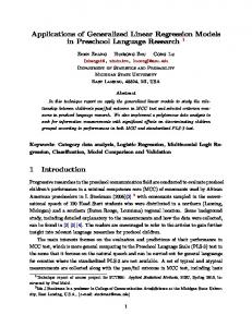

![APPLICATIONS OF MULTIMEDIA FORENSICS DISSERTATION ... [PDF]](https://m.moam.info/img/260x300/applications-of-multimedia-forensics-dissertation-_647debae098a9ef61c8b4640.jpg)
![APPLICATIONS OF MULTIMEDIA FORENSICS DISSERTATION ... [PDF]](https://m.moam.info/img/260x300/applications-of-multimedia-forensics-dissertation-_647d959a098a9eb9638b465d.jpg)