Recent work by Tomov and Dongarra [Tomov and Dongarra 2009] shows ... Section 2 describes the new algorithm for m-Hessenberg reduction. ..... The old value of the element a .... Process block A(i) = A(1 : n, z : z + b â 1) with k = z + m â 1 by ...... Composer 2011.4.191 with multithreaded Intel R Math Kernel Library 10.3.
Efficient generalized Hessenberg form and applications Nela Bosner, Zvonimir Bujanovi´c, and Zlatko Drmaˇc
This paper proposes an efficient algorithm for reducing matrices to the generalized Hessenberg form by unitary similarity, and recommends using it as a preprocessor in a variety of applications. As an illustration of its power, two cases from control theory are analyzed in detail: a solution procedure for a sequence of shifted linear systems with multiple right hand sides (e.g. evaluating transfer function of a linear time invariant (LTI) dynamical system, with multiple inputs and outputs, at many complex values) and computation of the staircase form. The proposed algorithm for the generalized Hessenberg reduction introduces two levels of aggregation of Householder reflectors, thus allowing efficient BLAS 3 based computation. Another level of aggregation is introduced when solving many shifted systems by processing the shifts in batches. Numerical experiments confirm that the proposed methods have superior efficiency. Categories and Subject Descriptors: G1 [Numerical Analysis]: Numerical Linear Algebra— Error Analysis; G4 [Mathematical Software]: —Reliability; Robustness General Terms: Algorithms, Reliability, Theory Additional Key Words and Phrases: Hessenberg form, shifted linear systems, staircase algorithm, transfer function
1.
INTRODUCTION
Hessenberg form belongs to the tools of trade of numerical linear algebra. We say that H ∈ Rn×n is m-Hessenberg matrix, m < n, if Hij = 0 for all i, j = 1, . . . , n such that i > j + m. Any A ∈ Rn×n can be written as A = U HU T , where U is orthogonal and H is m-Hessenberg form of A. Such a generalized Hessenberg structure naturally arises e.g. in the block Arnoldi algorithm, and it is very frequent in the computational control. For instance, the controller Hessenberg form of (A, B) ∈ Rn×n ×Rn×m is (H, ( R0 )) = (QT AQ, QT B), where Q is orthogonal, H is m-Hessenberg and R is upper triangular. For computing the standard (1-)Hessenberg form, the state of the art software package LAPACK [Anderson et al. 1992] contains an optimized subroutine xGEHRD. Recent work by Tomov and Dongarra [Tomov and Dongarra 2009] shows that on a hybrid CPU/GPU parallel computing machinery, a considerable speedup over xGEHRD is possible; see also [Tomov et al. 2010]. In a distributed parallel computing environment, ScaLAPACK [ScaLAPACK 2009] provides parallel subroutines PxGEHRD. For the controller Hessenberg form, the computational control library SLICOT [SLICOT 2009] contains the subroutine TB01MD, which also computes the m-Hessenberg form. Unlike xGEHRD, the subroutine TB01MD does not use aggregated transformations (block reflectors). As a consequence, its low flop–to–memory– reference ratio cannot provide optimal efficiency. Our goal is high performance CPU and CPU/GPU software for the generalized Hessenberg form and its applications. We are in particular interested in the computational control applications and contributions to the control library SLICOT. In the first stage of the development, we give detailed block CPU implementaACM Journal Name, Vol. V, No. N, Month 20YY, Pages 1–0??.
·
2
tions. Section 2 describes the new algorithm for m-Hessenberg reduction. In §3, we apply the m-Hessenberg form as a preprocessor and improve the efficiency of the staircase reduction, which is one of the structure revealing canonical forms of LTI systems [Dooren 1979]. In §4, we show how to use the m-Hessenberg form and a variant of incomplete RQ factorization to compute C(σI − A)−1 B very efficiently for possibly large number of complex values σ. Numerical experiments in §5 show that the new algorithms provide superior performances. The second part of this work, in a separate report [Bosner et al. 2011], contains parallel hybrid CPU/GPU implementations of the algorithms from this paper. A BLOCK ALGORITHM FOR M -HESSENBERG FORM
2.
As with the QR and the 1-Hessenberg LAPACK routines, the main idea for a faster m-Hessenberg algorithm is to partition the n × n matrix1 A into blocks of b consecutive columns, A = (A(1) A(2) . . . A(l) ), l = dn/be. Each of the leading l − 1 blocks carries b columns, while the last one contains the remaining n − (l − 1)b ones. After determining suitable block size b, the blocks are processed one at a time, from left to right, and the computation is organized to enhance temporal and spatial data locality. In particular, some transformations are postponed until the very last moment in which the updated content is actually needed for the next step. Accumulated transformations are then applied in a block fashion, thus increasing the flop count per memory reference. Many details and tricks are involved, and this section contains the blueprints of the new algorithm. 2.1
Processing a single block
Processing a block consists of constructing b Householder reflectors that annihilate appropriate elements in each of the block’s columns. For the i-th block A(i) = (i) (i) (i) (a1 a2 . . . ab ), define a sequence of Householder reflectors: for j = 1, 2, . . . , b, let (i) Hj = I −τj vj vjτ be the Householder reflector such that the vector Hj Hj−1 · · · H1 aj has zeros as its (k + j + 1)-th, (k + j + 2)-th, . . . , n-th element (with an offset k that will be a function of i and b). Here τj is a scalar and vj is a vector such that vj (1 : k + j − 1) = 0 and vj (k + j) = 1. These vectors are stored in the matrices Vj = (v1 v2 . . . vj ). (The introduction of the Vj matrices is for explanatory purposes only.) As in xGEHRD, the non-trivial elements of the vectors vj are stored in the matrix A in places of entries that have been zeroed by the Hj ’s. In our description of the algorithm, we overwrite the initial data, thus there will be no “time stepping” index in our notation. To set the stage for the new algorithm and to introduce necessary notation, we briefly describe block reflectors. For more details we refer the reader to [Schreiber and van Loan 1989]. Proposition 1. The product Qj = H1 H2 . . . Hj can be represented as Qj = I − Vj Tj Vjτ , where Tj is an upper triangular j × j matrix. Proof. The construction of Tj is inductive: we first set V1 = (v1 ), T1 = τ1 , and 1 For
the sake of brevity, we describe only the real case. The algorithm is easily extended, mutatis mutandis, to complex matrices. ACM Journal Name, Vol. V, No. N, Month 20YY.
·
3
τ then we easily verify that, for t+ = −τj Tj−1 Vj−1 vj , it holds τ Qj = Qj−1 Hj = (I − Vj−1 Tj−1 Vj−1 ) · (I − τj vj vjτ ) � � Tj−1 t+ = I − (Vj−1 vj ) · · (Vj−1 vj )τ . 0 τj � � Tj−1 t+ Thus, setting Tj = completes the proof. 0 τj
Once the block is processed, we will have to update A ← Qτ AQ = (I − V T τ V τ )A(I − V T V τ ) = (I − V T τ V τ )(A − Y V τ ) ,
(1)
where V = Vb , T = Tb , Q = Qb and Y = AV T . The auxiliary matrix Y will be used for fast update of the matrix A “from the right-hand side” (A ← A − Y V τ ). Proposition 2. The matrices Yj = Y (:, 1 : j) = AVj Tj satisfy: � τ vj + Avj ) . Y1 = τ1 Av1 ; Yj = Yj−1 τj (−Yj−1 · Vj−1
(2)
Proof. Starting with Y1 = τ1 Av1 and using Proposition 1, we have � � � � Tj−1 t+ Yj = A · Vj−1 vj · = AVj−1 Tj−1 AVj−1 t+ + τj Avj 0 τj � τ τ vj + Avj ) . (3) = (since t+ = −τj Tj−1 Vj−1 vj ) = Yj−1 τj (−Yj−1 · Vj−1 In order to compute the reflector that annihilates the elements in the j-th column of the block, we must have already updated this part of the matrix A with the accumulated product Hj−1 · · · H1 . To that end, we use Yj−1 , following (1). Note that computing the reflectors requires only the elements of A in the rows from (k + 1)-st on – thus the update will also require only the elements of Yj−1 with the same row indices. The processing of a single block is outlined in Algorithm 1 and the details are given in §2.1.1-§2.1.4. 2.1.1
(i)
Updating aj (k+1 : n) from the right. In line 4 of Algorithm 1, the column
(i)
aj (k + 1 : n) is updated by the transformation from the right. The details of this update are given in Algorithm 2 and in Figure 1, which illustrates the situation in the case n = 15, m = 2 and the block size b = 5. The current block A(i) is shaded (i = 2); the parameter k is equal to (i − 1) · b + m = 7. The elements of a particular (i) column aj are shown as diamonds and filled circles (j = 4). All elements below (i)
the m-th subdiagonal in the columns to the left of aj have already been set to zero by the algorithm, and our goal now is to use a Householder reflector and zero (i) out those elements of the column aj that are shown as filled circles. Prior to that, we have to apply to this column the previously generated block τ reflector I − Vj−1 Tj−1 Vj−1 from both the left and the right. During the block (i)
processing, only the row indices k + 1 : n of aj will be updated – the remaining indices are not involved in computation of the Householder reflectors for the current block. For the same reason, only the rows k + 1 : n of Yj−1 and Vj−1 will be
ACM Journal Name, Vol. V, No. N, Month 20YY.
·
4
Algorithm 1: Processing of a block to reduce it to m-Hessenberg form Input: block A(i) , block size b, index k Output: partially updated block A(i) , transformation matrices Y and T , auxiliary array T AU ; details in §2.1.1, 2.1.2, 2.1.3. for j = 1, 2, . . . , b do if j > 1 then (i) 3 Update aj (k + 1 : n):
1 2
(i)
(i)
5 6 7 8 9 10 11
(i)
τ aj (k + 1 : n) = aj (k + 1 : n) − (Yj−1 Vj−1 )(k + 1 : n, k + j − m);
4
end
τ τ Vj−1 from the left; Multiply aj (k + 1 : n) with I − Vj−1 Tj−1 (i)
Generate the elementary reflector Hj to annihilate aj (k + j + 1 : n); Set T AU (j) = τj , and compute Yj (k + 1 : n, j); Compute Tj (:, j); end Compute Y (1 : k, 1 : b); (i)
aj = A(:, k + j − m)
k k+1
��������F������ ��������F������ ��������F������ �������F������ ������F������ �����F������ ����F������ ���F������ ��F������ �F������ F������ u������ u������ u������ u������ A
—
��� ��� ��� ��� ��� ��� ��� ��� ��� ��� ��� ��� ��� ��� ��� Yj−1
·
� � � � � � � 1 � 1 p �1 pp ppp ppp ppp ppp ppp
τ
k+j−m
Vj−1
(i)
Fig. 1: Updating column aj (k + 1 : n) from the right (line 4 in Algorithm 1)
referenced. The horizontal dashed line separates the rows 1 : k and k + 1 : n of all matrices in the figure. All action takes place below this line. The non-trivial elements of the matrix Vj−1 are shown as – these are actually stored in places of the elements of A(i) that have already been zeroed out. All elements above the ones in the matrix Vj−1 are zero. Note that the j-th column of the block A(i) is the ((i − 1) · b + j = k + j − m)-th column of the original matrix (i) A. Thus, updating the column aj involves only the row k + j − m of the matrix Vj−1 – the shaded one in Figure 1. In fact, what is needed from this row are the leading j − m − 1 elements stored in A(i) (k + j − m, 1 : j − m − 1), and a single
p
ACM Journal Name, Vol. V, No. N, Month 20YY.
·
5
Algorithm 2: Details of line 4 in Algorithm 1 4.1 4.2 4.3 4.4
if j > m then (i) temp = aj−m (k + j − m); (i)
aj−m (k + j − m) = 1; Call xGEMV (BLAS 2) to compute (i)
4.5
(i)
aj (k + 1 : n) = aj (k + 1 : n)− �τ Yj−1 (k + 1 : n, 1 : j − m) · A(i) (k + j − m, 1 : j − m) ;
(i)
aj−m (k + j − m) = temp; end
k+j−1
� � � � � � � 1 � p 1 �1 pp ppp ppp ppp ppp ppp
��� �� � ·
τ
·
Vj−1
Tj−1
� � � � � � � 1 � p 1 �1 pp ppp ppp ppp ppp ppp Vj−1
τ
F F F F F F F F F F F u u u u
·
(i)
aj
(i)
Fig. 2: Updating column aj (k + 1 : n) from the left
element 1 (thus the trick with introducing 1 in line 4.3 in Algorithm 2). (i)
2.1.2 Updating aj (k + 1 : n) from the left. The details of the implementation of line 5 in Algorithm 1 are given in Algorithm 3, and illustrated in Figure 2. (i) τ The lines 5.2 and 5.3 compute the product Vj−1 aj . This multiplication is carried out in two phases: first, we multiply the triangular block Vj−1 (k + 1 : k + j − 1, 1 : j − 1) using the xTRMV routine. This routine can be deployed to “pretend” as if the lower triangular matrix has ones on its diagonal without explicitly looking up matrix elements, enabling us to avoid the temporary backup of elements of A(i) which occupy that place. (This triangular block of Vj−1 is between the dashed and the wavy line in Figure 2.) Then the rectangular block Vj−1 (k + j : n, 1 : j − 1) (i) multiplies the rest of vector aj . (i)
τ τ In line 5.4, the vector Tj−1 Vj−1 aj
is formed, and lines 5.5–5.7 complete the ACM Journal Name, Vol. V, No. N, Month 20YY.
·
6
Algorithm 3: Details of line 5 in Algorithm 1 (i)
Copy aj (k + 1 : k + j − 1) to T (1 : j − 1, j); 5.2 Call xTRMV (BLAS 2) to compute �τ T (1 : j − 1, j) = A(i) (k + 1 : k + j − 1, 1 : j − 1) · T (1 : j − 1, j); 5.3 Call xGEMV to compute �τ (i) T (1 : j − 1, j) = T (1 : j − 1, j) + A(i) (k + j : n, 1 : j − 1) · aj (k + j : n); τ 5.4 Call xTRMV to compute T (1 : j − 1, j) = Tj−1 · T (1 : j − 1, j); 5.5 Call xGEMV to compute
5.1
(i)
(i)
aj (k + j : n) = aj (k + j : n) − A(i) (k + j : n, 1 : j − 1) · T (1 : j − 1, j); 5.6 Call xTRMV to compute T (1 : j − 1, j) = A(i) (k + 1 : k + j − 1, 1 : j − 1) · T (1 : j − 1, j); 5.7
(i)
(i)
aj (k + 1 : k + j − 1) = aj (k + 1 : k + j − 1) − T (1 : j − 1, j);
Algorithm 4: Details of line 8 in Algorithm 1 (i)
(i)
temp = aj (k + j); aj (k + j) = 1; 8.2 Call xGEMV to compute 8.1
(i)
Yj (k + 1 : n, j) = A(k + 1 : n, k + j : n) · aj (k + j : n); 8.3 Call xGEMV to compute �τ (i) Tj (1 : j − 1, j) = A(i) (k + j : n, 1 : j − 1) · aj (k + j : n); 8.4 Call xGEMV to compute Yj (k + 1 : n, j) = Yj (k + 1 : n, j) − Yj−1 (k + 1 : n, :) · Tj (1 : j − 1, j); 8.5 Scale Yj (k + 1 : n, j) by multiplying it with τj = T AU (j); transformation by multiplying that vector by Vj−1 from the left. 2.1.3 Other details of block processing. The line 7 is a single call of the LA(i) PACK routine xLARFG. The Householder vector is stored in aj (k + j + 1 : n), while the scalar τj is stored in an auxiliary array T AU as the element T AU (j). Next, in line 8, we append a column to Yj−1 to define Yj as in (2). Note that (i) aj (k + j + 1 : n) now contains the non-trivial part of the j-th elementary Householder vector. Algorithm 4 gives the details. Line 8.2 is the only line in the loop of the block processing algorithm that references elements of A outside of the current block A(i) . This is also the only line which deals with a matrix of dimension O(n) × O(n); all others have at least one τ dimension of block size b or less. Line 8.3 computes the product Vj−1 vj – observe that vj (1 : k + j − 1) = 0, so we can disregard the rows 1 to k + j − 1 of the matrix (i) Vj−1 . The old value of the element aj (k + j), whose backup copy is in line 8.1, (i)
can be restored after the update of the next column aj+1 . All that is now left to do in order to complete the matrix Tj is to re-scale the current content of its last column by T AU (j), and to multiply it by Tj−1 from the left by using yet another call to xTRMV. Finally, we show how to compute the first ACM Journal Name, Vol. V, No. N, Month 20YY.
· ����� ����� ����� ����� ����� ����� ����� ����� ����� ����� ����� ����� ����� ����� ����� Y
=
��������������� ��������������� ��������������� �������������� ������������� ������������ ����������� ���������� ��������� �������� ������� ������ ����� ����� �����
·
� � � � � � � 1 � p1 1 � pp 1 � ppp �1 pppp ppppp ppppp ppppp
A
V
7
����� ���� ��� �� � ·
T
Fig. 3: Updating first k rows of Y
k rows of Y , outside of the main loop in Algorithm 1 (line 11): Algorithm 5: Details of line 11 in Algorithm 1 Copy A(1 : k, k + 1 : k + b) to Y (1 : k, 1 : b); Call xTRMM (BLAS 3) to compute Y (1 : k, 1 : b) = Y (1 : k, 1 : b) · A(i) (k + 1 : k + b, 1 : b); 11.3 Call xGEMM (BLAS 3) to compute Y (1 : k, 1 : b) = Y (1 : k, 1 : b) + A(1 : k, k + b + 1 : n) · A(i) (k + b + 1 : n, 1 : b); 11.4 Call xTRMM to compute Y (1 : k, 1 : b) = Y (1 : k, 1 : b) · T ;
11.1 11.2
�
In Figure 3, the region below the elements denoted by in the current block (shaded) of the matrix A has been zeroed out. It now stores the non-trivial part of the matrix V (elements denoted by ). Multiplication by the matrix V from the right in lines 11.2 and 11.3 is once again split into triangular and rectangular parts. Line 11.3 references elements not in the current block. Note that only the columns k + 1 : n of the matrix A (the ones to the right of the vertical dashed line) are referenced while updating Y , because of the zero-pattern in V .
p
2.1.4 The concept of mini-blocks. The first m columns of a block do not need to be updated from the right since the corresponding rows of the matrices Vj−1 are zero. Moreover, if m is greater than or equal to the block size, then the updates from the right are not needed at all within the current block.2 When m is less than the block size, this fact permits another variant of Algorithm 1 in which: (1) The block is split into several disjoint “mini-blocks”, each (except maybe the last one) consisting of m consecutive columns. (2) In each “mini-block”, column by column is updated only from the left, and the appropriate elements are annihilated. 2 We
are indebted to Daniel Kressner [Kressner 2010] for pointing this out; a similar concept is also used in [Bischof et al. 2000] for the reduction of a symmetric matrix to the tridiagonal form. The mini-blocks are also successfully used in [Karlsson 2011]. ACM Journal Name, Vol. V, No. N, Month 20YY.
·
8
Algorithm 6: Processing of a block by using mini-blocks to reduce it to mHessenberg form Input: block A(i) , block size b, index k Output: partially updated block A(i) , transformation matrices Y and T , auxiliary array T AU for j = 1, 2, . . . b do if j > 1 then (i) τ τ 3 Update aj (k + 1 : n) only from the left by applying I − Vj−1 Tj−1 Vj−1 ; 4 end 1 2
5 6 7 8 9 10 11
12 13 14
(i)
Generate the elementary reflector Hj to annihilate aj (k + j + 1 : n); Compute Tj (:, j); if j mod m = 0 or j = b then cM ini = m or (b mod m); // current miniblock size nM ini = min{b − j, m}; // next miniblock size Compute Yj (k + 1 : n, j − cM ini + 1 : j); Call xGEMM to update the entire next miniblock from the right: A(i) (k + 1 : n, j + 1 : j + nM ini) = A(i) (k + 1 : n, j + 1 : j + nM ini) − (Yj Vjτ )(k + 1 : n, j + 1 : j + nM ini); end end Compute Y (1 : k, 1 : b);
τ (3) A “mini-reflector” Qm = I − Vm Tm Vm is aggregated from m annihilations.
(4) After processing of the “mini-block”, the block reflector Qj+m is updated: � Vj+m = �Vj Vm � ; Tj Tjm τ Tj+m = , Tjm = −Tj Vj Vm Tm ; (4) 0 Tm � τ Yj+m = Yj (−Yj Vj Vm + AVm )Tm . (5) The next m columns of A are updated from the right; these columns are then declared the new current “mini-block”. Note that, in order to update all columns in the next “mini-block” from the right, one only needs the elements of Y that lie in the current and previous “mini-blocks”, see line 4.4 in Algorithm 2. Thus, an update from the right of the entire next “miniblock” and the appropriate part of the matrix Y may be computed after all columns in the current “mini-block” have been annihilated. The details are worked out in Algorithm 6 which, for m > 1, makes better use of BLAS 3 operations than the original Algorithm 1 and thus provides better performance. The minimum size of m where this variant is more effective depends on the user’s machine setup – on our machine, for m ≥ 3 the speedup was already notable. (See subsection 5.1 for timing results that illustrate a considerable improvement due to the modification described in Algorithm 6.) ACM Journal Name, Vol. V, No. N, Month 20YY.
·
��������5 �5 �5 �0 �0 �0 �0 �0 ��������5 �5 �5 �0 �0 �0 �0 �0 ��������5 �5 �5 �0 �0 �0 �0 �0 �������5 �5 �5 �0 �0 �0 �0 �0 ������5 �5 �5 �0 �0 �0 �0 �0 �����5 �5 �5 �0 �0 �0 �0 �0 ����5 �5 �5 �0 �0 �0 �0 �0 ������0 �0 �0 �0 �0 �����0 �0 �0 �0 �0 ����0 �0 �0 �0 �0 ���0 �0 �0 �0 �0 ��0 �0 �0 �0 �0 �0 �0 �0 �0 �0 �0 �0 �0 �0 �0 �0 �0 �0 �0 �0 A
—
�5 �5 �5 �� �5 �5 �5 �� �5 �5 �5 �� �5 �5 �5 �� �5 �5 �5 �� �5 �5 �5 �� �5 �5 �5 �� ����� ����� ����� ����� ����� ����� ����� ����� Y
·
� � � � � � � 51 � p5 51 � p5 p5 51 � 1 p0 p0 p0 00 p0 p0 p0 p0 01 p0 p0 p0 p0 p0 p0 p0 p0 p0 p0 p0 p0 p0 p0 p0
9
τ
V
Fig. 4: Updating the matrix A from the right, A = A − Y V τ .
This completes the description of the block processing algorithm. We now turn our attention to the global algorithm on the block level. 2.2
The outer loop
Figure 4 shows the update A = A − Y V τ , where Y and V are computed during the last block processing (the last block A(i) is shaded). This update only affects the columns k + 1 : n of A – the ones to the right of the vertical dashed line. Only the elements of A that are encircled or boxed have yet to be updated, since the block processing has already updated A(i) (k + 1 : n, 1 : b). The boxed elements of A will be updated by subtracting the product of Y with the boxed part of V . Since the elements of V above the ones are all zeros and V is stored in A(i) , the appropriate part of A(i) has to be replaced with zeros and ones in order to use the xGEMM routine for the multiplication. The encircled elements of A will be updated by subtracting the product of encircled elements of Y with the triangular matrix of encircled elements in V . The Block Algorithm 7 at first just stores all of the block’s reflectors, instead of annihilating columns one by one and applying the resulting reflector to the entire matrix A each time. Only after a block is processed, the whole batch of its reflectors is applied to A, first from the left and then from the right. This brings several important performance benefits into play. The first one is the localization of memory referencing: in the point version, the algorithm has to reference elements of A that are “far away” (in terms of memory addresses) from the current column when applying the reflectors, for each column being annihilated. On the other hand, the block version mostly references only elements local to the block being processed. Elements “far away”, i.e. the ones outside of that block are referenced only after all of the block’s reflectors have already been computed. If the block size is chosen to fit into the cache memory, there will be much less cache misses during the computation of all the reflectors and less data fetching from the slower main memory. The second advantage is the more effective transformation A 7→ Qτ AQ. If Q were a single Householder reflector, one could only use BLAS ACM Journal Name, Vol. V, No. N, Month 20YY.
10
·
Algorithm 7: Block algorithm for reduction to the m-Hessenberg form Input: n × n matrix A, block size b, bandwidth m Output: A converted to m-Hessenberg form for z = 1, 1 + b, 1 + 2 · b, 1 + 3 · b, . . . do i = (z − 1)/b + 1; 3 Process block A(i) = A(1 : n, z : z + b − 1) with k = z + m − 1 by Algorithm 6; 1 2
4 5
6 7 8
// Apply block reflector from the right: Backup the upper triangle of A(i) (k + b − m + 1 : k + b, b − m + 1 : b) into matrix temp and replace it with the upper triangle of identity matrix; Call xGEMM to compute �τ A(1 : n, z + b : n) = A(1 : n, z + b : n) − Y · A(i) (k + b − m + 1 : n, 1 : b) ; Restore temp to upper triangle of A(i) (k + b − m + 1 : k + b, b − m + 1 : b); Call xTRMM to compute �τ temp = Y (1 : k, 1 : b − m) · A(i) (k + 1 : k + b − m, 1 : b − m) ; A(1 : k, k + 1 : z + b − 1) = A(1 : k, k + 1 : z + b − 1) − temp;
// Apply block reflector from the left: Call xLARFB to apply block reflector (V, T ) from left onto A(k + 1 : n, z + b : n); 10 end 9
2 operations to apply the transformation, whereas transformation routines such as xLARFB use the more efficient BLAS 3 operations (e.g. xGEMM, xTRMM), taking advantage of the underlying block reflector structure of Q. 3.
THE STAIRCASE FORM
The m-Hessenberg form can be used for efficient computation of other useful canonical forms. For instance, the controller Hessenberg form of (A, B) ∈ Rn×n × Rn×m is easily computed in two steps: first compute the QR factorization B = Q1 ( R0 ), update A to A(1) = QT1 AQ1 , and compute the m-Hessenberg form H = QT2 A(1) Q2 . Then, the transformation Q = Q1 Q2 produces QT AQ = H, QT B = ( R0 ). We now turn our attention to detecting whether the system is controllable and to determining its controllable part. A numerically reliable method for such task is the computation of a staircase form. n×m , Theorem 3. [Dooren 1979] For a pair (A, B), where A ∈ Rn×n and � B∈R τ τ n×n there exists an orthogonal matrix Q ∈ R such that Q B Q AQ equals
�
¯ A¯11 B 0 0
A¯12 A¯22
� ≡
X1 Aˆ11 0 X2 .. .. . . 0 0 0 0
ACM Journal Name, Vol. V, No. N, Month 20YY.
Aˆ12 . . . Aˆ22 . . . . .. . .. . . . Xk ... 0
Aˆ1k Aˆ1,k+1 Aˆ2k Aˆ2,k+1 .. .. . . Aˆkk Aˆk,k+1 0 Aˆk+1,k+1
,
·
11
Algorithm 8: Computing a staircase form with a full system matrix A Input: the system (A, B) ˆ B) ˆ in the staircase form Output: the system (A, � ¯ ¯ 1 Compute RRD B = U B 0 , where B has full row rank ρ1 ; τ 2 Update A = U AU ; 3 Set prev = 0, curr = ρ1 , i = 1; 4 while curr < n do 5 Set Z = A(curr + 1 : n, prev + 1 : prev + ρi ); 6 if Z is a zero matrix then 7 break: the system is uncontrollable; 8 end � 9 Compute RRD Z = U Z0¯ , where Z¯ has full row rank ρi+1 ; 10 Update from left: A(curr + 1 : n, prev + 1 : n) = U A(curr + 1 : n, prev + 1 : n); 11 Update from right: A(1 : n, curr + 1 : n) = A(1 : n, curr + 1 : n)U τ ; 12 prev = curr, curr = curr + ρi+1 , i = i + 1; 13 end � ˆ = A, B ˆ = B¯ ; 14 Set A 0 where each matrix Xi is of order ρi × ρi−1 and has a full row rank ρi (we set ρ0 = m). The initial system (A, B) is controllable if and only if A¯22 = Aˆk+1,k+1 is Pk ¯ ¯ void, i.e. i=1 ρi = n. Otherwise, (A11 , B) is the controllable part of (A, B). If the matrix A has no structure, then a common way of computing the staircase form is shown in the Algorithm 8. A series of rank-revealing decompositions of the sub-matrices is computed. By a rank-revealing decomposition� (RRD) of the matrix Z ∈ Rp×q , p ≥ q, we consider any factorization Z = U Z0¯ , where U is orthogonal and Z¯ has a full row rank. To make the staircase algorithm more efficient, usually a rank-revealing QR-factorization is used instead of the more reliable, but slower singular value decomposition. The SLICOT routine AB01ND implements a staircase algorithm which uses the classical QR-factorization with Businger–Golub pivoting and an incremental rank estimator. Note that most of those pivoted QR factorizations run on tall matrices. To compute Xi (line 9), the factorization of a matrix with at least n−(i−1)m rows is required. The corresponding updates (lines 10 and 11) transform the sub-matrix of order at least (n−(i−1)m)×(n−(i−1)m). Assuming the usual case m � n, we see that many of these updates are actually on O(n) × O(n) sub-matrices. 3.1
A new scheme
We propose a novel algorithm for computing the staircase form in which the system is first transformed into the controller Hessenberg form using the blocked algorithm described in §2. Then, we use Algorithm 9, specially tailored for the generalized Hessenberg structure. Compared to the Algorithm 8, performance is gained because of these differences, which are due to the m-Hessenberg form of the system matrix: —RRDs in line 9 are computed on matrices with h rows. The number h is initially ACM Journal Name, Vol. V, No. N, Month 20YY.
12
·
equal to m, and may increase by at most m − 1 in each pass through the whileloop. Therefore, we expect that RRDs are computed on matrices having only O(m) rows. —Update in line 10 transforms a submatrix of order O(m) × O(n). —Update in line 11 transforms a submatrix of order O(n) × O(m).
�����FFFF������ �����FFFF������ �����FFFF������ �����FFFF������ ����FFFF������ uuF5 F5 F5 F5 EEEEEE uuF5 F5 F5 F5 EEEEEE uuF5 F5 F5 F5 EEEEEE uuF5 F5 F5 F5 EEEEEE FFF������ FF������ F������ ������ ����� ���� Fig. 5: A typical situation in the loop of Algorithm 9. RRD is computed on the submatrix •; elements ◦ are updated from the left, and elements � are updated from the right. Here n = 15, m = ρ0 = ρ1 = 3, ρ2 = 2.
4.
SHIFTED SYSTEMS AND TRANSFER FUNCTION
Hessenberg reduction is known to be an excellent preprocessing tool in solving shifted linear systems, in particular for evaluating the transfer function G(σ) = C(σI − A)−1 B + D of a LTI system (A, B, C, D) ∈ Rn×n × Rn×m × Rp×n × Rp×m at many values of complex scalar σ. Recently, it has been shown that using the controller Hessenberg form of (A, B) or (AT , C T ) allows for more efficient and numerically more consistent computation in the case min(m, p) = 1; for details and references see [Beattie et al. 2011]. Here we extend those ideas to the case min(m, p) > 1, where it is tacitly assumed that max(m, p) is small compared to n. Henry [Henry 1994] introduced the idea of using the RQ factorization (A−σI)U = T , where U is n × n unitary, and T is n × n upper triangular. Then, C(σI − A)−1 B = −(CU )(T −1 B), and the original problem reduces to matrix multiplication and backward substitutions using the upper triangular matrix T . It is immediately clear how the controller Hessenberg structure of (A, B) simplifies this computation. First, performing many RQ factorizations is more efficient if the matrix A is in Hessenberg form simply because part of the matrix is already zero. Next, m � −1 � � � � ˆ ˆ ˆ m Tˆ T B B T −1 B = , B= , T = n−m 0 0 0 ACM Journal Name, Vol. V, No. N, Month 20YY.
n−m � ∗ , ∗
·
13
Algorithm 9: Computing a staircase form of a system in controller Hessenberg form Input: the system (A, ( B0 )) in the controller Hessenberg form � ˆ Bˆ ) in the staircase form Output: the system (A, 0 � ¯ ¯ 1 Compute RRD B = U B 0 , where B has full row rank ρ1 ; 2 Update A from left: A(1 : m, 1 : n) = U τ A(1 : m, 1 : n); 3 Update A from right: A(1 : 2m, 1 : m) = A(1 : 2m, 1 : m)U ; 4 Set h = m, prev = 0, curr = ρ1 , i = 1; 5 while curr < n do 6 Set Z = A(curr + 1 : curr + h, prev + 1 : prev + ρi ); 7 if Z is a zero matrix then 8 break: the system is uncontrollable; 9 end � 10 Compute RRD Z = U Z0¯ , where Z¯ has full row rank ρi+1 ; 11 Update from left: A(curr + 1 : curr + h, prev + 1 : n) = U A(curr + 1 : curr + h, prev + 1 : n); 12 Update from right: A(1 : curr + h + m, curr + 1 : curr + h) = A(1 : curr + h + m, curr + 1 : curr + h)U τ ; 13 h = h + m − ρi+1 , prev = curr, curr = curr + ρi+1 , i = i + 1; 14 end ˆ = A, B ˆ = B; ¯ 15 Set A ˆ Tˆ−1 B), ˆ where Cˆ = (CU )(1 : p, 1 : m). Note that only and C(σI − A)−1 B = −C( ˆ the leading m×m matrix T of T is needed, which further simplifies the computation of the RQ factorization (both in number of flops and memory management); also, only a part of the transformed C is needed. In short, for each σ the computation ˆ is organized to compute only Tˆ and C. The RQ factorization is computed by Householder reflectors, U = H1 H2 · · · Hn−1 , where the i-th reflector Hi annihilates all subdiagonal elements in the (n − i + 1)th row. The reduction starts at the last and finishes at the second row. For i = n − m + 1, . . . , n − 1, during the update of the rows m, . . . , 2, the matrix Tˆ is built bottom-up and the back-substitution is done on the fly. 4.1
A point algorithm
We first describe an algorithm in which the Householder reflectors are computed and applied one by one. Since the matrix A is in the m-Hessenberg form, in each row we have to annihilate m entries. This means that the corresponding Householder vector has at most m + 1 nonzero elements. Further, the application of the corresponding Householder reflector affects only m + 1 columns of the matrices A − σI and C. Since we need only a part of the RQ factorization, at no point we need more than m + 1 columns of the transformed A − σI and of the transformed C. (The role of C is rather passive – it just gets barraged by a sequence of reflectors, designed to produce triangular structure of A − σI, and only Cˆ is wanted.) For this reason we introduce an auxiliary (p + n) × (m + 1) array Z which, at any moment, stores ACM Journal Name, Vol. V, No. N, Month 20YY.
·
14
m + 1 columns of the thus far transformed matrices C and A − σI. We can think of Z as a sliding window, moving from the last m + 1 columns to the left. Algorithm 10: A point algorithm for computing G(σ), where A and B are in the controller Hessenberg form. Input: (A, B, C, D) ∈ Rn×n × Rn×m × Rp×n × Rp×m ((A, B) in the controller Hessenberg form); complex scalar σ Output: G(σ) ≡ C(σI − A)−1 B + D 1 2 3 4 5 6 7 8 9 10 11 12 13 14 15 16
17 18
Z(1 : p, 1 : m) = C(1 : p, n − m + 1 : n); Z(p + 1 : p + n, 1 : m) = (A − σI)(1 : n, n − m + 1 : n); for k = n : −1 : m + 1 do Z(1 : p + k, 2 : m + 1) = Z(1 : p + k, 1 : m); Z(1 : p, 1) = C(1 : p, k − m); Z(p + 1 : p + k, 1) = (A − σI)(1 : k, k − m); ¯ such that Determine (m + 1) × (m + 1) Householder reflector H ¯ Z(p + k, 1 : m + 1)H = ( 0 0 · · · 0 ∗ ); Transform ¯ : m + 1, 1 : m); Z(1 : p + k − 1, 1 : m) = Z(1 : p + k − 1, 1 : m + 1)H(1 end ˆ = B; ˆ X for k = m : −1 : 2 do ¯ such that Determine k × k Householder reflector H ¯ = ( 0 0 · · · 0 ∗ ); Z(p + k, 1 : k)H ¯ Transform Z(1 : p + k − 1, 1 : k) = Z(1 : p + k − 1, 1 : k)H; ˆ ˆ Compute X(k, k : m) = X(k, k : m)/Z(p + k, k); Compute ˆ : k − 1, k : m) = X(1 ˆ : k − 1, k : m) − Z(p + 1 : p + k − 1, k) · X(k, ˆ X(1 k : m); end ˆ : p, 1 : m) is now stored in Z(1 : p, 1 : m) // C(1 ˆ // T is now stored in Z(p + 1 : p + m, 1 : m). ˆ 1 : m) = X(1, ˆ 1 : m)/Z(p + 1, 1); X(1, ˆ G(σ) = D − Z(1 : p, 1 : m) · X;
4.2
A block algorithm
Block algorithm for the RQ factorization by Householder reflectors is based on a special block representation of aggregated product of several reflectors. It is a wellknown technology, and we will adjust it to our concrete structure. We will use a “reversed” WY representation of the aggregated Householder reflectors, which is a modification of the WY form from [Bischof and Loan 1987]. Proposition 4. Let Hi = I − τi vi vi∗ be a Householder reflector, and let Uj = H1 H2 · · · Hj . Then Uj can be represented as Uj = I − Yj Vj∗ , where � � V1 = v1 , Y1 = τ1 v1 ; Vi = vi Vi−1 , Yi = τi Ui−1 vi Yi−1 , i = 2, . . . , j. ACM Journal Name, Vol. V, No. N, Month 20YY.
·
15
The correctness of the above representation is easily checked, and we will see later why this particular form is practical in our framework. Let nb denote the block size, i.e. the number of aggregated reflectors. Since nb consecutive transformations on nb rows touch m + nb consecutive columns of A − σI and C, we extend our auxiliary array Z, and define it as (p + n) × (m + nb ) to accommodate m + nb columns of the transformed matrices C and A − σI. The sliding window (array Z) will move to the left now with step nb : its last nb columns will be discarded, the leading m columns shifted to the right, and new nb columns from A−σI and C will be brought as the leading columns of Z. During this sliding, the number of rows of Z shrinks by nb at each step. Only the last nb rows of the current Z are needed to generate the reflector, and these pivotal parts of the sliding window are trapezoidal matrices sliding upwards along the diagonal of A − σI. The last m − 1 Householder reflectors which reduce the rows m, m − 1, . . . , 2 of the matrix A − σI compute the dense RQ factorization and for small m are applied as in the point algorithm. 4.2.1 Auxiliary: Trapezoidal to triangular reduction. We use an auxiliary RQ routine to reduce an nb × (m + nb ) upper trapezoidal matrix to triangular form by right multiplication by a sequence of Householder reflections, �0 0 0 x x x x� �x x x x x x x� 0 xxxxxx −→ 00 00 00 00 x0 xx xx . (5) 0 0 xxxxx 0 0 0 xxxx
000 0 0 0 x
In the global scheme, this trapezoidal matrix is an nb × (m + nb ) pivotal block of the auxiliary matrix Z. Most of the time we are not interested in the resulting triangle, but in the aggregated product of the reflectors, which will be packed in the reversed WY form and applied to only the part of the copy of the global array (stored in Z) that is needed in subsequent steps. Updates with Householder reflectors within the auxiliary routine are also done in the blocked manner. The current row which determines current Householder reflector, is not updated by previous reflectors from the block until it is needed. Prior to computing the current Householder vector, aggregated Householder reflectors from previous steps have to be applied to the current row. Moreover, we update only the part of the row that carries information needed to construct the reflector for the next step. Since the deployed reflectors are determined by Householder vectors with at most m + 1 nonzero elements (occupying consecutive positions), the matrix V is banded with bandwidth m + 1 and Y is lower trapezoidal: • 0 0 0 ? 0 0 0 •• 0 0
?? 0 0
0 ••• 0 0 •• 0 0 0 •
???? ???? ????
? ? ? 0 • • • 0 V = • • • •, Y = ? ? ? ?
(6)
Since an application of the block transformation I − Y V ∗ involves V ∗ , it is convenient to store V ∗ instead of V . Each time a new (m + 1)-dimensional Householder vector v is determined, the first m components of v ∗ are stored in places of m subdiagonal elements that are annihilated by the corresponding reflector. The Householder vector is scaled so that its last component is equal to one, and there is no need for storing it. This procedure is implemented in the LAPACK routine ACM Journal Name, Vol. V, No. N, Month 20YY.
16
·
xLARFG. Hence, combining (5) and (6), the normalized V ∗ is placed in the last nb rows of Z as follows: �• • • x x x x� Z(n + p − nb + 1 : n + p, 1 : m + nb ) ≡ Zblock = 00 •0 •• •• x• xx xx , 0 0 0 • • • x
where Z contains the last m + nb columns of A and C. Algorithm 11: Reduction of an nb × (m + nb ) upper trapezoidal block to the triangular form. Input: nb × (m + nb ) matrix block Zblock Output: V and Y such that Zblock (I − Y V ∗ ) is triangular as in (5) 1 2 3 4 5 6 7 8 9
10 11 12 13
14 15
V = 0(m+nb )×nb ; Y = 0(m+nb )×nb ; for k = nb : −1 : 1 do if k = nb then ¯ = I − τ v¯v¯∗ such Determine (m + 1) × (m + 1) Householder reflector H ¯ = ( 0 0 · · · 0 ∗ ); that Zblock (k, k : k + m)H Set V (k : k + m, k) = v¯; Set Y (k : k + m, k) = τ · v¯; else mb = min{nb − k, m}; Update of the current row: Call xGEMM twice to compute Zblock (k, k + 1 : k + m) = Zblock (k, k + 1 : k + m) − (Zblock (k, k + 1 : nb + m)· Y (k + 1 : nb + m, k + 1 : k + mb )) · V (k + 1 : k + m, k + 1 : k + mb )∗ ; ¯ = I − τ v¯v¯∗ such Determine (m + 1) × (m + 1) Householder reflector H ¯ that Zblock (k, k : k + m)H = ( 0 0 · · · 0 ∗ ); Set V (k : k + m, k) = v¯; Set Y (k : k + m, k) = τ · v¯; Call xGEMV twice to compute Y (k + 1 : nb + m, k) = Y (k + 1 : nb + m, k) − Y (k + 1 : nb + m, k + 1 : k + mb )· (V (k + 1 : k + m, k + 1 : k + mb )∗ · Y (k + 1 : k + m, k)); end end
The banded structure of the matrix V has been used to derive the lines 9 and 13 of Algorithm 11 from their original forms: line 9 of Algorithm 11. Zblock (k, k + 1 : k + m) = Zblock (k, k + 1 : k + m)− (Zblock (k, k + 1 : nb + m) · Y (k + 1 : nb + m, k + 1 : nb )) · V (k + 1 : k + m, k + 1 : nb )∗ line 13 of Algorithm 11. Y (k + 1 : nb + m, k) = Y (k + 1 : nb + m, k) − Y (k + 1 : nb + m, k + 1 : nb ) ·(V (k + 1 : k + m, k + 1 : nb )∗ · Y (k + 1 : k + m, k)) In both cases, we have multiplication of some submatrices of V and Y : Y (k + 1 : nb + m, k + 1 : nb ) · V (k + 1 : k + m, k + 1 : nb )∗ Since, for nb − k > m, V (k + 1 : k + m, k + m + 1 : nb ) = 0m×(nb −k−m) , we obtain the forms of these lines as presented in Algorithm 11. A similar modification will be used in Algorithm 12. ACM Journal Name, Vol. V, No. N, Month 20YY.
·
17
4.2.2 The outer loop. The global structure of the block algorithm is given in Algorithm 12. Algorithm 12: Block algorithm for computing G(σ), where A and B are in the controller Hessenberg form. Input: matrices A, B, C, D ((A, B) in the controller Hessenberg form); complex scalar σ, and block dimension nb Output: matrix G(σ) 1 lb = (n − m)/nb ; 2 mink = n − (lb − 1) · nb ; 3 Z(1 : p, 1 : m) = C(1 : p, n − m + 1 : n); 4 Z(p + 1 : p + n, 1 : m) = (A − σI)(1 : n, n − m + 1
5 6 7 8 9 10
11 12 13 14 15 16 17 18 19 20 21
: n); for k = n : −nb : mink do Z(1 : p + k, nb + 1 : m + nb ) = Z(1 : p + k, 1 : m); Z(1 : p, 1 : nb ) = C(1 : p, k − m − nb + 1 : k − m); Z(p + 1 : p + k, 1 : nb ) = (A − σI)(1 : k, k − m − nb + 1 : k − m); Compute V and Y by Algorithm 11, such that Z(p + k − nb + 1 : p + k, 1 : m + nb )(I − Y V ∗ ) is upper triangular; Call xTRMM and xGEMM to compute Z(1 : p + k − nb , 1 : m) = Z(1 : p + k − nb , 1 : m) − Z(1 : p + k − nb , 1 : m + nb )· (Y (1 : m + nb , 1 : m) · V (1 : m, 1 : m)∗ ); end l = n − lb · nb ; for k = l : −1 : m + 1 do Perform lines 4–8 of Algorithm 10; end ˆ = B; ˆ X for k = m : −1 : 2 do ˆ : m, 1 : m) as in lines 12–15 of Algorithm 10; Compute X(2 end ˆ 1 : m) = X(1, ˆ 1 : m)/Z(p + 1, 1); X(1, ˆ G(σ) = D − Z(1 : p, 1 : m) · X;
In the implementation of the Algorithm 12 we can also exploit the fact that V is banded with bandwidth m + 1 and Y is lower trapezoidal, hence the form of the implementation of line 10, which in the original reads: line 10 of Algorithm 12. Z(1 : p + k − nb , 1 : m) ← Z(1 : p + k − nb , 1 : m) − Z(1 : p + k − nb , 1 : m + nb ) · (Y · V (1 : m, 1 : nb )∗ ) Here we also assumed that nb ≥ m. Otherwise, V (1 : m, 1 : m) does not exist and we have the product Y V (1 : m, 1 : nb )∗ with smaller inner dimension. An estimate of additional workspace is as follows: • Two-dimensional array of dimension (m + nb ) × nb for storing the matrix Y . • One-dimensional array of dimension m for storing intermediate results in lines 9 and 13 of Algorithm 11 • Two-dimensional array of dimension (p + n − nb ) × m for storing intermediate ACM Journal Name, Vol. V, No. N, Month 20YY.
18
·
result in line 10 of Algorithm 12 • One-dimensional array of dimension p+m+nb −1 for storing intermediate results occurring in application of Householder reflector to a matrix in lines 14 and 17 of Algorithm 12 (lines 8 and 13 of Algorithm 10) ¯ Depending on m/n, X ¯ • Two-dimensional m × m array for storing the matrix X. ¯ appears after Y becomes obsolete. may be stored in place of Y , since X 4.2.3 Batch processing in case of multiple shifts. The second level of aggregation in the algorithm for solving shifted systems is processing the shifts in batches, see [Beattie et al. 2011]. There are several reasons for introducing this technique. First, we have to access the elements of the same matrices A and C for every shift. In each step of the outer loop, lines 7 and 8 are the same for every shift: the same nb columns of A and C are copied to the auxiliary array Z (except that different shifts are subtracted from the diagonal elements of A). Second, the most expensive operation in the algorithm, which is the update of Z with the Householder reflectors generated in Zblock (line 10), involves large amount of the same data for different shifts. These data are the first nb columns of Z, containing original elements of A and C, copied in lines 7 and 8. The main goal of shift aggregation is to avoid all these redundant operations. Let us assume that we evaluate the transfer function G(σi ) for ns different shifts σi , i = 1, . . . , ns . For all these shifts we will access all the elements of A and C only once, and we will perform one part of the update for all shifts simultaneously, as one call to xGEMM. Such approach will require much more memory for storing the auxiliary arrays, but it will reduce communication between different parts of the memory. The original array Z is now split in two parts: —The first part consists of the first nb columns of Z and is denoted by Z1 . This part is (almost) the same for all shifts and relates to the original elements of A and C. The “small” differences will be dealt with later. —The second part consists of the last m columns of Z that are specific to the shift σi , and is denoted by Z2 (i). These submatrices are the result of the update from the previous outer loop step, and are different for different shifts. We do not need to store the pivotal block Zblock after its reduction in Algorithm 11, and the Householder vectors which are generated in that block can be exploited immediately after the auxiliary routine implementing Algorithm 11 completes execution. Hence, we use the same nb × (m + nb ) array Zblock for all shifts. Finally, we will need the matrices Y (i) obtained from Algorithm 11 for different shifts σi . The actual placing of these matrices in the workspace will be described later, after some details of the new algorithm are explained. The update in line 10 of Algorithm 12 is now divided into two parts: one part dealing with shift specific arrays Z2 (i) and the other part dealing with Z1 which is common to all updates (for all shifts). Actually there is a “small” difference between the array Z1 and the first nb columns of the array Z from Algorithm 12, that was mentioned before. For Z1 to be identical in all updates it cannot include shifts, and that is not the case with Z. A shift is subtracted from the diagonal elements of Z(p + k − nb − m + 1 : p + k − nb , 1 : m), which is m × m bottom-left submatrix of the part of Z involved in update in the k-th outer loop step. Thus, ACM Journal Name, Vol. V, No. N, Month 20YY.
· single shift Zi
1
·
19
multiple shifts Z1
Z2 (i), i = 1, . . . , ns
Zblock
nb m
Y
Y (i), i = 1, . . . , ns
shifts
post-process Fig. 6: The layout of the auxiliary arrays within the working space.
Z1 will contain only elements of the original matrices A and C, and the shifts in the first m columns will be processed separately. The details of the update after reduction of the pivot block in case of multiple shifts are given in Algorithm 13. Line 10.4 in Algorithm 13 suggests the layout of the auxiliary arrays within the working space. We need only the first m columns of the matrices Y (i), so there is no need for storing all nb columns (under assumption nb ≥ m). Thus, submatrices Y (i)(1 : m + nb , 1 : m) should occupy m · ns consecutive columns as well as the matrices Z2 (i). We should also note that the result of the update (lines 10.1–10.4) is already placed on the right position for the next outer loop step, so that copying operation in line 6 of Algorithm 12 can be omitted. Similar techniques can be applied to the non-blocked part of the algorithm. 4.3
Descriptor systems
Algorithm 12 can be easily adapted for computing the transfer function G(σ) = C(σE − A)−1 B + D of a descriptor system. Here E ∈ Rn×n . For Algorithm 12 to be efficient, the matrices A, B and E have to be in the m-Hessenberg–triangular– triangular form. An efficient block algorithm for the m-Hessenberg–triangular– triangular reduction is described in [Bosner 2011]. The only changes required for descriptor systems in the m-Hessenberg–triangular– triangular form are in the lines 4, 8 and 14 (line 6 of Algorithm 10) of Algorithm 12 where specific columns of A − σI are copied to the auxiliary array Z. What we ACM Journal Name, Vol. V, No. N, Month 20YY.
·
20
Algorithm 13: Details of the update in case of aggregated shifts.
9 10.1 10.2
10.3
10.4
for k = n : −nb : mink do Initialize data; for 1 = 1 : ns do Perform necessary copying; Compute V (i) and Y (i) by Algorithm 11, such that Zblock (I − Y (i)V (i)∗ ) is upper triangular; Call xTRMM to compute Y (i)(1 : m + nb , 1 : m) = Y (i)(1 : m + nb , 1 : m) · V (i)(1 : m, 1 : m)∗ ; Call xGEMM to compute Z2 (i)(1 : p + k − nb , 1 : m) = Z1 (1 : p + k − nb , 1 : m) −Z2 (i)(1 : p + k − nb , 1 : m) · Y (i)(nb + 1 : nb + m, 1 : m); Z2 (i)(p + k − nb − m + 1 : p + k − nb , 1 : m) = Z2 (i)(p + k − nb − m + 1 : p + k − nb , 1 : m) + σ(i)Y (i)(1 : m, 1 : m) − σ(i)Im ; end Call xGEMM to compute ( Z2 (1) Z2 (2) · · · Z2 (ns ) )(1 : p + k − nb , 1 : m · ns) = ( Z2 (1) Z2 (2) · · · Z2 (ns ) )(1 : p + k − nb , 1 : m · ns)−Z1 (1 : p + k − nb , 1 : nb ) ·( Y (1)(1 : nb , 1 : m) Y (2)(1 : nb , 1 : m) · · · Y (ns )(1 : nb , 1 : m) ); end
actually do here is copying the specific columns of the matrix A to Z first, and then subtracting σ from the diagonal elements of A. We have to change only the second step and subtract the corresponding columns of E multiplied with σ in order to obtain columns of A − σE. Since E is upper triangular, this means that we have to update all elements in the current column of A except subdiagonal ones. 5.
NUMERICAL EXPERIMENTS
We have run a series of tests in order to assess the performances of the new softR XeonTM X5470 (quad-core), running at 3.33GHz ware. Our machine was a Intel with 8 GB RAM and 6+6MB of Level 2 cache memory, under Ubuntu Linux 8.10. R Fortran Compiler 11.0. We used -O3 optimization and The compiler was Intel R Math Kernel Library 10.1. All tests the BLAS and LAPACK from the Intel were run using the IEEE double precision and double complex arithmetic. The code was tested for correctness by computing the appropriate residuals and using SLICOT routines for reference values. 5.1
The m-Hessenberg reduction
We have compared the default point implementation found in the routine TB01MD from SLICOT with our new algorithms: blocked versions with and without the “mini-blocks”. Only the reduction of the matrix A to the m-Hessenberg form is tested, and the code for the QR-factorization of the matrix B is removed from the SLICOT routine, along with the corresponding similarity transformation of the matrix A. We note that the blocked implementation of these transformations would increase the gap between the algorithms even more. ACM Journal Name, Vol. V, No. N, Month 20YY.
· 50
10 m=1 m=5 m=20 m=100
time(no mini−blocks) / time(with mini−bloks)
time(TB01MD) / time(new mini−blocked algorithm)
60
21
40
30
20
10
9 8
m=5 m=20 m=100
7 6 5 4 3 2 1
0 0
1000
2000
3000
4000
5000
6000
7000
Dimension of A
(a) Speedup factors of the new (mini)blocked CPU routine relative to TB01MD.
0 0
1000
2000
3000
4000
5000
6000
7000
Dimension of A
(b) The blocked algorithm: with mini-blocks is faster
computation
Fig. 7: Comparisons of the new m-Hessenberg algorithms and TB01MD from SLICOT .
Figure 7a shows the speedup factors obtained by the the “mini-block” version of the CPU algorithm versus the SLICOT routine. The tests were run for a batch of matrices A with orders up to 6500 and various bandwidths m. The block size that performed well on our testing hardware was b = 64. As Figure 7a shows, the new algorithm can be more than 50 times faster than TB01MD. The significance of using the “mini-blocks” is shown in Figure 7b, where we compare two versions of our algorithms: the one using “mini-reflectors” and “mini-blocks” and the one updating each column of the block from the right prior to its annihilation. The blocking has more effect when m is larger. In fact, to compute 100-Hessenberg form of a 6000×6000 matrix our algorithm needs only about 1/9 of the time needed for computing the 1-Hessenberg form! One could use this fact to design an algorithm for successive band removal: in order to reduce a matrix to 1-Hessenberg, it is first very quickly reduced to e.g. 100-Hessenberg, and then using a similar process this intermediate matrix is further reduced to a 1-Hessenberg form. However, our attempts to design such an algorithm have failed so far: reduction from a 100Hessenberg form to a 1-Hessenberg form simply takes too long! In the symmetric case, this scheme is successful; see [Bischof et al. 2000]. (See also [Karlsson 2011].) 5.2
Reduction to the staircase form
We ran a number of numerical tests to demonstrate the efficiency of the Algorithm 9 compared to the Algorithm 8. Both algorithms used the same SLICOT routine MB03OY for RRDs; this routine implements a blocked rank-revealing QR algorithm using the Businger–Golub pivoting. We randomly generated systems (A B) of various orders and ran the staircase reduction algorithms. Figure 8 shows that the new algorithm performs up to 19 times faster than the original one. (The timings for the new algorithm include both the reduction to the controller–Hessenberg form and the subsequent transformation into the staircase form.) 5.3
Evaluation of the transfer function
Extensive numerical testing was performed for random systems with various values of n and m; in our tests we set p = m. We have compared the SLICOT routine ACM Journal Name, Vol. V, No. N, Month 20YY.
·
22
time(AB01ND) / time(new staircase algorithm)
20 18 16
m=1 m=5 m=20 m=100
14 12 10 8 6 4 2 0 0
1000
2000
3000
4000
5000
6000
7000
Dimension of A
Fig. 8: The staircase reduction: comparison of Algorithm 9 and AB01ND from SLICOT .
TB05AD to our new blocked CPU algorithm for transfer function computation, using r = 1000 random complex shifts. The routines were executed as follows:
time(TB05AD) / time(new multishift algorithm)
12
10
8
6
4 m=1 m=5 m=10 m=20
2
0 0
1000
2000
3000
4000
5000
6000
7000
Dimension of A
(a) Speedup factors of the new blocked CPU routine relative to TB05AD.
time(new singleshift algorithm) / time(new multishift algorithm)
our routines. CPU implementation of the reduction to the controller Hessenberg form was executed once followed by 1000 executions of our blocked CPU algorithm for computing G(σ); SLICOT routine TB05AD. at first the routine TB05AD was executed with the parameter INITIA=’G’, indicating that the matrix A is a general matrix, and without balancing and eigenvalues calculations (parameter BALEIG=’N’). This was followed by 999 executions of TB05AD with INITIA=’H’ indicating that the matrix A is in the upper Hessenberg form, which is computed using DGEHRD from LAPACK.
3.5
3
2.5
2
1.5 m=1 m=5 m=10 m=20
1
0.5 0
1000
2000
3000
4000
5000
6000
7000
Dimension of A
(b) Aggregation of shifts improves the block algorithm.
Fig. 9: Comparisons of the new transfer function algorithm and TB05AD from SLICOT .
The block size in our CPU algorithm was set to nb = 64, which was in most cases the optimal block size for our routine. The results presented in Figure 9a confirm that our block algorithm for evaluating the transfer function is generally faster than the corresponding SLICOT routine TB05AD. Figure 9b demonstrates ACM Journal Name, Vol. V, No. N, Month 20YY.
·
23
that aggregation of shifts significantly contributes to the efficiency (we aggregated ns = 256 shifts). Although its efficiency decreases as m increases, we can conclude that, as the dimension n grows, the efficiency of our routines is increasing. We finally note that obvious modifications apply for the cases of purely real shifts, or complex conjugate pairs of shifts. 5.4
Results on a different machine
R XeonTM E5620 We run the same test on the different machine with 2 × Intel (4 cores), running at 2.40GHz with 23.5 GB RAM and 12+12MB of Level 3 cache R Fortran memory, under Scientific Linux release 6.0. The compiler was Intel R Math Kernel Library 10.3. We Composer 2011.4.191 with multithreaded Intel obtained slightly weaker speedups than previously shown. The new m-Hessenberg algorithm was up to 32 times faster than TB01MD from SLICOT, for m = 100. When comparing the new staircase reduction algorithm to AB01ND from SLICOT, the best speedup factors were 8.7 for m = 1 and 16 for m = 20. The best achieved speedup factors of the new blocked transfer function routine relative to TB05AD from SLICOT were 3.7 for m = 20 and 10 for m = 1.
REFERENCES Anderson, E., Bai, Z., Bischof, C., Demmel, J., Dongarra, J., Croz, J. D., Greenbaum, A., Hammarling, S., McKenny, A., Ostrouchov, S., and Sorensen, D. 1992. LAPACK users’ guide, second edition. SIAM, Philadelphia, PA. ˇ, Z., and Gugercin, S. 2011. A note on shifted Hessenberg systems and Beattie, C., Drmac frequency response computation. ACM Transactions on Mathematical Software 38, 2. Bischof, C., Lang, B., and Sun, X. 2000. A framework for symmetric band reduction. ACM Transactions on Mathematical Software (TOMS) 26, 4, 581–601. Bischof, C. and Loan, C. F. V. 1987. The WY Representation for Products of Householder Matrices. SIAM J. Sci. Stat. Comput. 8, 1, s2–s13. Bosner, N. 2011. Algorithms for simultaneous reduction to the m-Hessenberg–Triangular– Triangular form. Tech. rep., University of Zagreb. ´, Z., and Drmac ˇ, Z. 2011. Efficient generalized Hessenberg form on a Bosner, N., Bujanovic hybrid CPU/GPU machine. Tech. rep., University of Zagreb. Dooren, P. M. V. 1979. The computation of Kronecker’s canonical form of a singular pencil. Linear Algebra and Appl. 27, 122–135. Henry, G. 1994. The shifted Hessenberg system solve computation. Tech. Rep. 94–163, Center for Applied Mathematics, Cornell University, NY. Karlsson, L. 2011. Scheduling of parallel matrix computations and data layout conversion for HPC and multi-core architectures. Ph.D. thesis, Department of Computing Science, Ume˚ a University, Sweden. Kressner, D. 2010. Personal communication. ScaLAPACK. 2009. http://www.netlib.org/scalapack/. Schreiber, R. and van Loan, C. 1989. A storage–efficient WY representation for products of Householder transformations. SIAM J. Sci. Stat. Comput. 10, 1, 53–57. SLICOT. 2009. The control and systems library. http://www.slicot.org/. Tomov, S. and Dongarra, J. 2009. Accelerating the reduction to upper Hessenberg form through hybrid GPU-based computing. Tech. rep., UT-CS-09-642, University of Tennessee, LAPACK Working note 219. Tomov, S., Nath, R., and Dongarra, J. 2010. Accelerating the reduction to upper Hessenberg, tridiagonal, and bidiagonal forms through hybrid GPU-based computing. Parallel Computing 36, 645–654. ACM Journal Name, Vol. V, No. N, Month 20YY.