transmitters to the destination are assumed to be either error-free or fully protected with ...... encoded observation vector of sensor i with length k, BPSK modulated version .... to trigger a fire alarm system or light-detectors that are used to turn on road lights at ...... The red line shows the upper bound on the overall system BER.
DISTRIBUTED ADAPTIVE ALGORITHM DESIGN FOR JOINT DATA COMPRESSION AND CODING IN DYNAMIC WIRELESS SENSOR NETWORKS
By Abolfazl Razi B.S. Sharif University of Technology, 1999 M.S. Tehran Polytechnic, 2001
A DISSERTATION Submitted in Partial Fulfillment of the Requirements for the Degree of Doctor of Philosophy (in Electrical Engineering)
The Graduate School The University of Maine May 2013
Advisory Committee: Ali Abedi, Associate Professor of Electrical and Computer Engineering, Advisor, Mauricio P. Da Cunha, Professor of Electrical and Computer Engineering, Nuri Emanetoglu, Assistant Professor of Electrical and Computer Engineering, Anthony Ephremides, Professor of Electrical and Computer Engineering, University of Maryland, Donald M. Hummels, Professor of Electrical and Computer Engineering
LIBRARY RIGHTS STATEMENT
In presenting this dissertation in partial fulfillment of the requirements for an advanced degree at The University of Maine, I agree that the Library shall make it freely available for inspection. I further agree that permission for “fair use” copying of this dissertation for scholarly purposes may be granted by the Librarian. It is understood that any copying or publication of this dissertation for financial gain shall not be allowed without my written permission.
Date:
Signature: Abolfazl Razi
DISTRIBUTED ADAPTIVE ALGORITHM DESIGN FOR JOINT DATA COMPRESSION AND CODING IN DYNAMIC WIRELESS SENSOR NETWORKS
By Abolfazl Razi Dissertation Advisor: Dr. Ali Abedi An Abstract of the Dissertation Presented in Partial Fulfillment of the Requirements for the Degree of Doctor of Philosophy (in Electrical Engineering) May 2013 Robust error recovery and data compression algorithms are desirable in Wireless Sensor Networks (WSN), while pose significant implementation challenges due to the dynamic nature of networks and limited available resources at each node. Several near optimal algorithms have been developed to realize Distributed Joint Source and Channel Coding (D-JSCC) performing both compression and error recovery tasks. However, majority of the reported techniques are too complex to be implemented in tiny sensor nodes. In this dissertation, a D-JSCC algorithm is proposed for WSN, which to the best of our knowledge, is less complex than previously reported methods. The idea is to exploit the existing correlation among sensors observations to eliminate transmission errors. The algorithm is general in the sense that it is applicable to a wide variety of analog and discrete sources without affecting quantization and digitization blocks. In this distributed algorithm, the sensors compress their data collectively and transmit to a central data fusion center without the need for inter-sensor communications. The algorithm is robust to sensor failures and stays operational even with only one active sensor.
A novel bi-modal decoder is proposed to constantly track the network state; e.g. channel conditions, observation accuracy, and the number of nodes. The decoder switches between two iterative and non-iterative modes based on the network state to maintain the overall data recovery performance at the highest possible level, while reducing the decoding complexity by avoiding unnecessary computations. Sensors observation accuracies can be extracted in real-time from the received data, hence no prior estimation is required at the destination. The algorithm can easily be scaled, since the decoding complexity grows linearly with the number of sensors. Furthermore, an optimal bundling policy is proposed to combine sensor measurements into transmit packets such that the end to end latency is minimized. This solution considerably reduces data collection delivery in time sensitive sensor applications such as remote surgery and air traffic control systems. The results of this low-complexity algorithm not only improves the performance of data aggregation in sensor networks, but also provides a criterion to determine required sensor density in a data field to achieve a desired reliability level.
DISSERTATION ACCEPTANCE STATEMENT
On behalf of the Graduate Committee for Abolfazl Razi, I affirm that this manuscript is the final and accepted dissertation. Signatures of all committee members are on file with the Graduate School at the University of Maine, 42 Stodder Hall, Orono, Maine. Submitted for graduation in May 2013.
Signature:
Date: Dr. Ali Abedi, Associate Professor, Electrical and Computer Engineering
ii
c 2013 Abolfazl Razi
All Rights Reserved
iii
DEDICATIONS
I dedicate this dissertation to my dear wife Fatemeh and sweeteheart daughter Rihanna.
iv
ACKNOWLEDGMENTS
Firstly, I would like to express my utmost gratitude to Prof. Ali Abedi, who has been an excellent advisor. His excellent supervision was perfectly guided me throughout this research. I learned a lot from him in how to conduct a successful research and present my idea and think for future applications. His brilliant thinking capabilities, broad vision about the wireless networks and innovative ideas have always inspired me. I want to sincerely thank him for his unending support during my PhD. He has gave me the opportunity of visiting University of Maryland during his sabbatical leave, where I gained an invaluable team working experience. He also encouraged me to participate in proposal writing activities to develop required skills for my future academic career. His advisory was extraordinary and I am always thankful for him. I am very grateful for my committee members Prof. Anthony Ephremides, Prof. Donald Hummels, Prof. Mauricio da Cunha and Prof. Nuri Emanetoglu for their great helps and service. Their comments on my dissertation tentative and oral presentation significantly contributed to the quality of this work. I specially thank Prof. Ephremides for all I learned from him during auditing his class on multi-user communications and our collaboration at the University of Maryland. I would like to take the chance to appreciate my other professors Prof. Vetelino, Prof. Kotecki and Prof. Aumman, from whom I learned a lot during my course work. The always were very kind and patiently answered my unending questions. I owe my success to my dear family. A special feeling of gratitude to my parents for raising me, and their continually support during my life. They prepared everything for my success and I will ever be thankful for them. I sincerely appreciate my lovely wife Fatemeh, who has been the best support for me. I was very lucky to meet her. She always have been very kind, supportive and patient during my PhD. She was my best friend and my best lab-mate too. She is a brilliant individual and her points and comments on my work were always very helpful. I also like to express my love to v
my sweet daughter Rihanna, who gave me a joyful life. She always energized me to work harder. I remember many nights that Fatemeh and Rihanna had not slept and were waiting to have a family dinner. My love goes to my dear family forever. My thanks go to my friends and lab mates Fred, Joel, Kayvan, Mojtaba, Kale, Peter and Dylan for their constructive discussions. They helped me to collect real-field data and develop practical test platforms and get familiar with some related software and hardware packages. I appreciate many other anonymous people who have directly or indirectly contributed to this work. Finally, I appreciate my sponsors, University of Maine, Maine Space Grant Consortium, National Aeronautics and Space Administration (NASA) and SPX Communication Technologies Corporation for financially supporting this work.
vi
TABLE OF CONTENTS
DEDICATIONS........................................................................................... iv ACKNOWLEDGMENTS............................................................................... v LIST OF TABLES ....................................................................................... xi LIST OF FIGURES..................................................................................... xii LIST OF ACRONYMS ................................................................................xvi
Chapter 1. INTRODUCTION ..................................................................................... 1 1.1. Motivations ...................................................................................... 1 1.2. Distributed Algorithm Design For Joint Compression and Transmission ...... 3 1.3. Contributions to the Current Open Problems........................................... 5 1.4. Dissertation Organizations .................................................................. 6 2. BACKGROUND AND PRELIMINARIES ..................................................... 9 2.1. Introduction ..................................................................................... 9 2.2. Multi-terminal Coding: an Information Theoretic Review ......................... 9 2.3. Direct vs Indirect Coding...................................................................16 2.4. Remote Sensing ...............................................................................16 2.5. The Chief Executive Officer Problem ...................................................16 2.5.1. The Rate Distortion Region of the CEO problem ...........................21 2.5.2. Quadratic Gaussian CEO Problem ..............................................22 2.5.3. Generalizations of the CEO Problem ...........................................23 2.5.4. Notes on the CEO Rate Distortion Function ..................................25 2.6. Distributed Coding ...........................................................................25 2.6.1. Joint Coding vs Distributed Coding .............................................25
vii
2.6.2. Rate Region for Coding of Two Correlated Sources ........................31 2.7. Practical Distributed Coding Design ....................................................33 2.7.1. Successive and Parallel Decoding ...............................................33 2.7.2. Robustness to Sensor Failure......................................................35 2.7.3. Structured Distributed Source Coding ..........................................36 2.7.4. Syndrome Based Structured Codes..............................................38 2.8. Channel Coding ...............................................................................39 2.8.1. Practical Channel Codes............................................................41 2.8.2. Block Codes and Convolutional Codes.........................................41 2.8.3. Source Coding Using Channel Codes ..........................................42 2.8.3.1. Syndrome Based DSC Using LDPC Codes ..........................43 2.8.3.2. Using LDPC Codes with Puncturing to Realize DSC .............44 2.8.3.3. DSC Using Turbo Codes ..................................................45 2.9. Distributed Joint Source Channel Codes ...............................................46 3. DISTRIBUTED JOINT SOURCE-CHANNEL CODING FOR BINARY CEO PROBLEM ......................................................................................49 3.1. Introduction ....................................................................................49 3.2. Preliminary Definitions .....................................................................50 3.3. System Model .................................................................................52 3.4. Distributed Coding for Sensors with Correlated Data...............................57 3.4.1. Random Interleaver ..................................................................57 3.4.2. RSC Encoders.........................................................................57 3.4.3. Puncturing Method ..................................................................58 3.4.4. DSC for Heterogeneous Mode....................................................60 3.4.5. DSC for Homogeneous Modes ...................................................61 3.5. Decoder Structure ............................................................................61 3.5.1. Correlation Extraction Method ...................................................65 viii
3.5.2. Summary of Modifications to Decoding Algorithm ........................68 3.6. Performance Analysis .......................................................................69 3.7. Optimum Number of Sensors .............................................................70 3.8. Summary of Contributions .................................................................78 4. CONVERGENCE ANALYSIS....................................................................80 4.1. Introduction ....................................................................................80 4.2. Analysis Framework .........................................................................82 4.2.1. Modified EXIT Charts Analysis..................................................83 4.2.2. EXIT Chart Derivation Method ..................................................88 4.3. Bi-modal Decoder Design..................................................................97 4.4. Numerical Results ............................................................................98 4.5. Summary of Contributions ............................................................... 100 5. DISTRIBUTED CODING FOR TWO-TIERED CLUSTERED NETWORKS.... 102 5.1. Introduction .................................................................................. 102 5.2. Two-tiered Network Model .............................................................. 103 5.2.1. Relaying Mode...................................................................... 104 5.2.2. Inner Channel Model.............................................................. 106 5.3. Performance Analysis ..................................................................... 108 5.3.1. Inner Channel BER Performance .............................................. 109 5.3.2. Overall System BER Performance............................................. 117 5.4. Numerical Results .......................................................................... 119 5.5. Summary of Contributions ............................................................... 123 6. DELAY MINIMAL PACKETIZATION POLICY ......................................... 125 6.1. Introduction .................................................................................. 125 6.2. Different Delay Sources in WSN....................................................... 126 6.2.1. Impact of Packet Length on End-to-End Latency ......................... 127
ix
6.2.2. Transmission Parameter Tuning................................................ 128 6.3. Packet Transmission Model.............................................................. 129 6.4. Packetization Module...................................................................... 131 6.5. Delay Optimal Packetization Policy ................................................... 136 6.5.1. Stability Condition................................................................. 138 6.5.2. Expected Waiting Time........................................................... 139 6.5.3. Packet Formation Delay .......................................................... 140 6.5.4. Optimum Packetization Interval Criterion................................... 141 6.6. Delay Performance Analysis ............................................................ 142 6.7. Summary of Contributions ............................................................... 144 7. CONCLUDING REMARKS .................................................................... 146 REFERENCES.......................................................................................... 152 APPENDIX A. PROOF OF THEOREMS FOR THE PROPOSED D-JSCC SCHEME............................................................................ 172 APPENDIX B. PROOF OF THEOREMS FOR DELAY MINIMAL PACKETIZATION POLICY................................................................. 183 BIOGRAPHY OF THE AUTHOR ................................................................ 186
x
LIST OF TABLES
Table 2.1. Joint probability mass function of two correlated symbols X1 and X2 . .....26 Table 2.2. Implementation of encoder f1 using Gray coding. ...............................29 Table 2.3. Probability mass function of E and mapping of encoder f2 . ...................29 Table 2.4. Distributed Coding by binning symbol X2 into 4 bins. ..........................30 Table 3.1. Variable definitions. .......................................................................51 Table 3.2. Function definitions. ......................................................................52 Table 5.1. Optimum power allocation for different SNR values. .......................... 116
xi
LIST OF FIGURES
Figure 2.1. Multi-terminal source coding. .........................................................10 Figure 2.2. Slepian-Wolf coding rate region for two correlated sources. ..................13 Figure 2.3. Multi-terminal source coding with direct and indirect observations. ........17 Figure 2.4. System model of the CEO problem...................................................19 Figure 2.5. Many help one problem: one sensor observes the source directly and the rest of sensors observe indirectly. ................................................24 Figure 2.6. Robust multi-terminal coding with multiple descriptions. .....................24 Figure 2.7. Illustration of three coding methods including independent coding, joint coding and distributed coding. ..................................................28 Figure 2.8. Rate region for independent, joint and distributed coding. .....................32 Figure 2.9. Parallel and successive decoding for the CEO problem.........................34 Figure 2.10. Source coding based on random binning and joint typicality. ...............37 Figure 2.11. Using LDPC codes to implement syndrome-based distributed source coding. ...........................................................................44 Figure 2.12. Using LDPC codes with puncturing to implement distributed source coding as proposed in [1]. .............................................................45 Figure 2.13. Distributed source coding using turbo codes with different compression methods. ............................................................................47 Figure 3.1. System model: a binary source is observed by a cluster of N sensors. .....53 Figure 3.2. Binary symmetric channel with input S, output X, and crossover probability β. ...............................................................................54 Figure 3.3. Employed RSC encoder. Cosing rate is : R(c) = 21 . .............................58 Figure 3.4. Distributed coding: D-PCCC scheme is used to estimate the binary data source, S observed by a cluster of N sensors. ..............................60 Figure 3.5. Modified MTD utilized at destination to decode the received frames. ......62 xii
Figure 3.6. Comparison of different decoding schemes for 3 sensors with correlated data (β = 0.01). ....................................................................70 Figure 3.7. Comparison of BER performance of the modified MTD with known and self-estimated observation error parameters (β = 0.05)...................71 Figure 3.8. BER performance of modified MTD vs BSC crossover probability for different number of sensors at SN R = −6 dB...............................72 Figure 3.9. The rate distortion function for a binary CEO problem with two sensors and logarithmic loss measure. ...............................................73 Figure 3.10. Communication channel from source to destination: Cascade of BSC broadcast channels and parallel Gaussian channels. ....................74 Figure 3.11. Information capacity of system vs observation accuracy (BSC crossover probability) and channel quality (SNR) for 4 sensors. ...........75 Figure 3.12. Information capacity of system vs observation accuracy (BSC crossover probability) and channel quality (SNR) for 4 sensors. ...........76 Figure 3.13. Analysis and simulation results for the impact of the number of sensors on the BER Performance (β = 0.01). ...................................78 Figure 4.1. Simplified block diagram of the proposed encoder/decoder structure for two sensors. ............................................................................83 Figure 4.2. Mutual information between the channel observation LLRs and the source data as a function of variance σ 2 and observation error β.............88 Figure 4.3. Empiricial distribution of the extrinsic LLRs. .....................................90 Figure 4.4. Conditional pdf of extrinsic LLRs in a MTD with complete and incomplete observation accuracies (N = 4, β = 0.2, σ = 5)..................92 Figure 4.5. Modified EXIT charts for the extreme case of complete observation accuracy (β = 0, Eb /N0 = 1dB).....................................................94
xiii
Figure 4.6. Modified EXIT charts for different observation accuracies (Number of sensors is 2). ............................................................................95 Figure 4.7. Convergence region of iterative decoding algorithm in terms of the channel SNR and sensors observation error parameter β. ......................98 Figure 4.8. Proposed bi-modal parallel-structure MTD decoder. ............................99 Figure 4.9. BER performance comparison of the iterative and non-iterative decoders (Number of sensors = 8, β = 0.1). .................................... 100 Figure 4.10. BER performance comparison of the proposed scheme with the similar codes. ........................................................................... 101 Figure 5.1. System model for two-tiered double-sink wireless sensor network. ....... 104 Figure 5.2. Simplified system model for a single cluster in a two-tiered doublesink wireless sensor network. ........................................................ 104 Figure 5.3. Channel coefficients for the communication links from sensors to the base station via two supernodes. .................................................... 106 Figure 5.4. Empirical pdf and Gaussian approximation of the noise term n12 with (sr)
parameters pe
= 0.1 and σg1 = σg2 = 1. ....................................... 111
Figure 5.5. Inner channel error probability vs power allocation parameter α. ......... 120 P for different noise levels...... 121 Figure 5.6. Optimum power allocation vs SNR: N1 +N 2
Figure 5.7. End-to-end probability of error for the system with 4 sensors. ............. 122 Figure 5.8. Comparison of system performance for different number of supernodes, with and without STBC coding at supernodes (N=4). ................. 123 Figure 6.1. System Model: arrival symbols are bundled into packets and are scheduled for transmission............................................................ 129 Figure 6.2. Packetization policy: Ki symbols of length N arrived in the ith interval of duration T form a packet of length Ki N + H. ......................... 131
xiv
Figure 6.3. Probability mass function of service time (λT = 10, H = N = 20, β = 0.01, C = 1). ....................................................................... 133 Figure 6.4. Coefficient of variance of the service time vs packetization time and different PERs (N = 16, H = 30, λ = 10)....................................... 142 Figure 6.5. Expected delay vs packetization time for different PERs (N = 16, H = 30, λ = 10). ................................................................... 144 Figure 6.6. Optimal packetization time vs packet header size for different PERs (N = 8, λ = 10). ........................................................................ 144
xv
LIST OF ACRONYMS
AF
Amplify and Forward . . . . . . . . . . . . . . . . . . . . . . . . . . . . . . . . . . . . . . . . . . . . . . . . . 8
ARQ
Automatic Repeat reQuest . . . . . . . . . . . . . . . . . . . . . . . . . . . . . . . . . . . . . . . . . . . 125
AWGN Additive White Gaussian Noise . . . . . . . . . . . . . . . . . . . . . . . . . . . . . . . . . . . . . . . . 22 ATM
Asynchronous Transfer Mode . . . . . . . . . . . . . . . . . . . . . . . . . . . . . . . . . . . . . . . . 127
BER
Bit Error Rate . . . . . . . . . . . . . . . . . . . . . . . . . . . . . . . . . . . . . . . . . . . . . . . . . . . . . . . . . 7
BMI
Bitwise Mutual Information . . . . . . . . . . . . . . . . . . . . . . . . . . . . . . . . . . . . . . . . . . . 86
BP
Belief Propagation . . . . . . . . . . . . . . . . . . . . . . . . . . . . . . . . . . . . . . . . . . . . . . . . . . . . 41
CDMA Code Division Multiple Access . . . . . . . . . . . . . . . . . . . . . . . . . . . . . . . . . . . . . . . . 59 CEO
Chief Executive Officer . . . . . . . . . . . . . . . . . . . . . . . . . . . . . . . . . . . . . . . . . . . . . . . . 4
CRC
Cyclic Redundancy Check . . . . . . . . . . . . . . . . . . . . . . . . . . . . . . . . . . . . . . . . . . . . . 8
CRV
Continuous-Valued Random Variable . . . . . . . . . . . . . . . . . . . . . . . . . . . . . . . . . . . 50
cpdf
cumulative probability distribution function . . . . . . . . . . . . . . . . . . . . . . . . . . . . . 50
CSI
Channel State Information . . . . . . . . . . . . . . . . . . . . . . . . . . . . . . . . . . . . . . . . . . . 108
D-JSCC Distributed Joint Source-Channel Coding . . . . . . . . . . . . . . . . . . . . . . . . . . . . . . . 5 D-STBC Distributed Space Time Block Codes . . . . . . . . . . . . . . . . . . . . . . . . . . . . . . . . . . 7 DF
Decode and Forward . . . . . . . . . . . . . . . . . . . . . . . . . . . . . . . . . . . . . . . . . . . . . . . . . 105
DMC
Discrete Memoryless Channel . . . . . . . . . . . . . . . . . . . . . . . . . . . . . . . . . . . . . . . . . 55
DMF
DeModulate and Forward . . . . . . . . . . . . . . . . . . . . . . . . . . . . . . . . . . . . . . . . . . . . . . 7
DRV
Discrete-Valued Random Variable . . . . . . . . . . . . . . . . . . . . . . . . . . . . . . . . . . . . . . 50
DSC
Distributed Source Coding . . . . . . . . . . . . . . . . . . . . . . . . . . . . . . . . . . . . . . . . . . . . . 1
DTC
Distributed Turbo Codes . . . . . . . . . . . . . . . . . . . . . . . . . . . . . . . . . . . . . . . . . . . . . . 98
EXIT
Extrinsic Information Transfer . . . . . . . . . . . . . . . . . . . . . . . . . . . . . . . . . . . . . . . . . . 7 xvi
FCFS First Come First Serve . . . . . . . . . . . . . . . . . . . . . . . . . . . . . . . . . . . . . . . . . . . . . . . . . 8 FDMA Frequency Division Multiple Access . . . . . . . . . . . . . . . . . . . . . . . . . . . . . . . . . . . 59 FEC
Forward Error Correction . . . . . . . . . . . . . . . . . . . . . . . . . . . . . . . . . . . . . . . . . . . . . 39
GSM
Global System for Mobile Communications . . . . . . . . . . . . . . . . . . . . . . . . . . . . 127
ID
Identification Data . . . . . . . . . . . . . . . . . . . . . . . . . . . . . . . . . . . . . . . . . . . . . . . . . . . 126
i.i.d
independent and identically distributed . . . . . . . . . . . . . . . . . . . . . . . . . . . . . . . . . 10
LDGM Low Density Generator Matrix Codes . . . . . . . . . . . . . . . . . . . . . . . . . . . . . . . . . . 41 LDPC Low Density Parity Check Codes . . . . . . . . . . . . . . . . . . . . . . . . . . . . . . . . . . . . . . 41 LT
Luby Transform . . . . . . . . . . . . . . . . . . . . . . . . . . . . . . . . . . . . . . . . . . . . . . . . . . . . . . 41
MA
Multiple Access . . . . . . . . . . . . . . . . . . . . . . . . . . . . . . . . . . . . . . . . . . . . . . . . . . . . . . 59
MAP
Maximum A Posteriori . . . . . . . . . . . . . . . . . . . . . . . . . . . . . . . . . . . . . . . . . . . . . . . . 42
MLD
Maximum Likelihood Detection . . . . . . . . . . . . . . . . . . . . . . . . . . . . . . . . . . . . . . . 65
MSE
Mean Square Error . . . . . . . . . . . . . . . . . . . . . . . . . . . . . . . . . . . . . . . . . . . . . . . . . . . 11
MT
Multi-Terminal . . . . . . . . . . . . . . . . . . . . . . . . . . . . . . . . . . . . . . . . . . . . . . . . . . . . . . . 9
MTD
Multi-branch Turbo Decoder . . . . . . . . . . . . . . . . . . . . . . . . . . . . . . . . . . . . . . . . . . . . 6
PCCC Parallel Concatenation of Convolutional Codes . . . . . . . . . . . . . . . . . . . . . . . . . . . 6 pdf
probability distribution function . . . . . . . . . . . . . . . . . . . . . . . . . . . . . . . . . . . . . . . . 50
PER
Packet Error Rate . . . . . . . . . . . . . . . . . . . . . . . . . . . . . . . . . . . . . . . . . . . . . . . . . . . 127
pmf
probability mass function . . . . . . . . . . . . . . . . . . . . . . . . . . . . . . . . . . . . . . . . . . . . . 50
RS
Reed-Solomon . . . . . . . . . . . . . . . . . . . . . . . . . . . . . . . . . . . . . . . . . . . . . . . . . . . . . . . 41
RV
Random Variable . . . . . . . . . . . . . . . . . . . . . . . . . . . . . . . . . . . . . . . . . . . . . . . . . . . . . 10
SAW
Surface Acoustic Wave . . . . . . . . . . . . . . . . . . . . . . . . . . . . . . . . . . . . . . . . . . . . . . 150
SISO
Soft Input Soft Output . . . . . . . . . . . . . . . . . . . . . . . . . . . . . . . . . . . . . . . . . . . . . . . . 62 xvii
SOC
System On Chip . . . . . . . . . . . . . . . . . . . . . . . . . . . . . . . . . . . . . . . . . . . . . . . . . . . . . . . 2
SOVA Soft Output Viterbi Algorithm . . . . . . . . . . . . . . . . . . . . . . . . . . . . . . . . . . . . . . . . . 42 TDMA Time Division Multiple Access . . . . . . . . . . . . . . . . . . . . . . . . . . . . . . . . . . . . . . . . 59 TS
Time Slot . . . . . . . . . . . . . . . . . . . . . . . . . . . . . . . . . . . . . . . . . . . . . . . . . . . . . . . . . . . 126
WEF
Weight Enumeration Function . . . . . . . . . . . . . . . . . . . . . . . . . . . . . . . . . . . . . . . . 117
WSN
Wireless Sensor Networks . . . . . . . . . . . . . . . . . . . . . . . . . . . . . . . . . . . . . . . . . . . . . . 1
ZMCGRV Zero-Mean Complex Gaussian Random Variables . . . . . . . . . . . . . . . . . . . 106
xviii
Chapter 1 INTRODUCTION
1.1 Motivations Distributed algorithms can address a variety of problems in dynamic systems at lower cost compared to centralized methods. One example of such problems is data acquisition, compression and transmission in time-varying wireless networks and Adhoc Wireless Sensor Networks (WSN). We are surrounded by a huge number of sensors. Buildings are equipped with fire sensors, smoke detectors, and surveillance camera systems. An airplane flies smoothly and stays safe benefiting from thousands of sensors measuring temperature, humidity, speed, acceleration, stress, air pressure, and elevation in different parts of engine, aircraft body, and cockpit. Any modern factory today is controlled by advanced sensing systems for safety and economical reasons. Biomedical sensors, health monitoring systems and remote surgery save thousands of lives every day. As these large-scale data networks grow and penetrate into various applications, the efficient use of natural resources such as frequency spectrum becomes even more critical. The more efficiently the limited available resources are used, the more advanced and higher quality services can be offered. The urgent need for these applications has attracted a large number of researchers to study the problem of data compression and efficient transmission techniques without compromising the quality of service in complex data networks [2]. A comprehensive study of this still ongoing research over several years reveals that the main attention of most research projects have been focused on the optimality of developed techniques in a pure theoretical evaluation framework. Efficient data compression techniques for correlated sources, the so called Distributed Source Coding (DSC) in the context of communication systems, have evolved in the past decades with development of several
1
intelligently designed algorithms [2]. However, due to the lack of focus on practical considerations, majority of these methods are not considered in practical system design and protocol development for commercial systems. For instance, the most currently available System On Chip (SOC) sensor platforms such as Telos B Motes, Stargate, Mica2, Tmote Sky and IBM cricket still stick with the traditional point-to-point independent coding following IEEE 802.15 series of standards in physical layer design and do not utilize recently proposed DSC schemes despite their proven promising performances [3–6]. The major reasons that has prevented the expected success of these DSC codes in practice are: • High complexity • Non-realistic assumptions • Static behavior The algorithms developed for DSC are so complex that their usage in tiny sensors with limited power and computational capabilities is very challenging. Non-realistic assumptions, although are necessary for performance evaluation in a theoretical study, should be avoided as much as possible in practical algorithm design. For instance, any multiple relay system that requires a full synchronization among the relay nodes will not become an appropriate candidate for ad-hoc networks. Likewise, the use of jointly Gaussian distributed assumption for correlated sources, existence of error-free instantaneous feedback channel, and prior knowledge about the correlation model induces a big gap between theoretical evaluations and practical results. A proper algorithm for very complex, crowded and dynamically changing networks should include two properties of distributed design and self-adaptation. This research is devoted to this purpose through designing distributed algorithms for compression and collection of correlated data in dynamically varying complex sensor networks. The proposed algorithms are supposed to constantly track the system conditions and adapt to the current situations. 2
The algorithms should be robust to node failures and simple enough for use in sensors with limited capabilities. This increases the chance of using the proposed algorithms in practical system design for current and future applications. 1.2 Distributed Algorithm Design For Joint Compression and Transmission A collection of sensors with a central data fusion unit and some intermediate relay nodes that communicate over wireless channels forms a WSN [7]. A wireless network, where all of the transmitters communicate directly with the base station is called Collocated Network [8]. This is a proper model for applications with small coverage area. In a large scale sensor network, where a sheer numbers of sensors collect data from a relatively large area, grouping sensors into several clusters has several advantages including but not limited to: lower power consumption, ease of scalability, lower maintenance cost, longer network life time and data communication efficiency. Moreover, clustering simplifies the algorithm development and analysis of the whole system behavior. Various clustering algorithms are proposed considering different limitations and performance metrics are proposed in the literature [9, 10]. Inside a cluster of sensors, due to the continuous nature of most environmental data fields such as temperature, humidity, and light, the observed field by adjacent sensors creates highly correlated data streams. This is called spatial correlation, which can be modeled with a closed form expression for some environmental data sources in terms of cluster size and relative distances of sensors [11]. One prevalently used technique is to model correlation among multiple observations with jointly Gaussian distributed random processes [12–14]. This does not cover the wide range of various source types and observation technologies. An approximate, but a more general model is considered in this research, where the observations are modeled using virtual Binary Symmetric Channels (BSC). This approximate model applies to binary sources as well
3
as discrete and continuous-valued sources with arbitrary observation models after digitization stage [15, 16]. It is well known for decades that considering the correlation among sensors and utilizing DSC can reduce the compression rate to as low as the joint entropy of correlated sources, which is much less than their sum entropy obtained through independent coding [17, 18]. Correlation among sensors are mainly due to observing a common shared data source [12, 19, 20]. An important variant of correlated observations arises when a common data source is observed by multiple sensors which is called the Chief Executive Officer (CEO) problem. This is in analogy to a problem, where the manager of a company individually interviews several partially trusted agents to get fairly assuring information about the company [21]. Remote sensing is one of the important practical applications of the CEO problem. This applies to a class of sensory systems, where sensors can not be placed at exact data source locations due to physical or environmental constraints. Hence, a cluster of sensors are placed at the proximity of a data source to secure a desired reliability. This problem has been throughly investigated from information-theoretic perspective and performance bounds are derived for some special cases, the most important of which is including jointly Gaussian distributed observations [22, 23]. These theoretical studies have been followed by efforts to develop practically efficient DSC schemes [2, 24, 25]. The first realization of DSC was introduced by Ramchandran, et. al. employing the Syndrom concept in a new coding scheme called DISCUS1 [26]. Afterwards, another variant of DSCs were developed based on the more powerful channel codes such as Low Density Parity Check Codes (LDPC) [27], Turbo Codes [28], [29], Irregular Repeat Accumulate (IRA) [30] , and Low Density Generator Matrix Codes (LDGM) [31]. 1
Distributed Source Coding Using Syndromes
4
Channel codes are widely used to facilitate data recovery in noisy environments by means of adding additional controlled redundancy to the transmit data. In practice, it is often advantageous to combine the DSC and the subsequent channel coding stages into a single step namely Distributed Joint Source-Channel Coding (D-JSCC) to reduce the computational complexity and implementation cost [32]. The most reported realizations of DJSCC are based on LDPC and Turbo like codes [18, 33–36]. 1.3 Contributions to the Current Open Problems Despite promising performance of the previously reported DJSCC schemes, a majority of them suffer from several drawbacks that make them inefficient for computationally constrained sensors. One limitation in prior works is assuming that some sensors have complete observation capabilities providing perfect side information to decode the other partially accurate sensors [26, 37]. In this research, we relax this limitation and consider incomplete observations for all sensors in the network. The second and more important constraint is the scalability issue of the codes. Some of the reported schemes are designed and analyzed for only two sensors [36]. Some others, even though support higher number of sensors, but are practically implementable only if the number of sensors are rather low [2, 15, 33, 35, 38]. Since the decoding complexity grows linearly with the number of sensors, our proposed scheme is easily scalable to an arbitrary number of sensors. Extension to any number of sensors is straightforward and does not require a radical redesign. Some of the reported codes yield only non-equal asymmetric rates [26], while the proposed scheme in this research supports both symmetric and asymmetric modes (equal and non-equal coding rates) by enabling per sensor coding rate adjustments capability. In contrast with syndrome-based techniques, the proposed scheme is robust to sensor failures and continues to decode as long as one or some of the sensors is operational in the system. Another noteworthy property of the proposed scheme is that prior information on the correlation model and
5
accuracy of the sensors are not needed, since the proposed decoding algorithm automatically extracts this information from the received data. The above mentioned advantages of the proposed technique are summarized as follows: • simplicity of encoder structure, • supporting both complete and incomplete observation accuracies, • low complexity of decoder (almost linearly grows with the number of sensors), • scalability to an arbitrary number of sensors, • flexibility of coding rate per sensor including both symmetric and asymmetric rates, • robustness to sensor failures, • no need for prior knowledge of correlation model. 1.4 Dissertation Organizations In chapter 2, a comprehensive review of formal definitions and reported results for various Multi Terminal (MT) coding scenarios with special emphasis on the CEO problem is provided. The previously reported D-JSCC schemes are also reviewed with mentioning their major drawbacks to present our motivation to develop practically applicable algorithms. An implementation-friendly DJSCC scheme for the binary CEO problem is proposed in chapter 3 based on the Parallel Concatenation of Convolutional Codes (PCCC) with a modified Multi-branch Turbo Decoder (MTD). The proposed iterative decoding algorithm extracts the correlation parameters from the received frames per each frame transmission cycle, hence can be used in applications with unknown or even time varying correlation models. Moreover, an approximate information-theoretic
6
analysis is derived to find the minimum number of sensors with certain observation accuracies to yield the minimum obtainable end-to-end estimation error, which was verified by numerical results. The results of this analysis can be used as an additional criterion for clustering algorithms in order to configure the network more efficiently and employ minimum number of sensors in each cluster. It is commonly agreed that in a MTD decoder, iteratively exchanging information between constituent decoders always enhances the system Bit Error Rate (BER) performance. In chapter 4, this presumption is revisited. Indeed, the usefulness of iterations is shown to be highly dependent on the certain system quality factors including the channel quality and sensors’ observation accuracies. Intuitively, iterative decoding seems to be better suited for sensors with low observation errors, where observations of different sensors are close enough to cause the iterative decoding algorithm to converge; otherwise the algorithm diverges. This conjecture is precisely formulated by introducing a new convergence analysis technique based on Extrinsic Information Transfer (EXIT) charts for MTD decoder with distributed encoders. This analysis led to design of a bimodal decoder that adaptively switches between two modes, iterative and non-iterative based on the system quality conditions to keep the BER performance as high as possible. The achieved BER is comparable to the more complex distributed LDPC codes and superior to previously reported distributed turbo codes under a fair comparison parameter set. Also, the decoding latency and power consumption is minimized by avoiding useless and even destructive additional iterations. In a traditional statically clustered two-tiered WSN, a cluster head (supernode) collects data from sensors inside a cluster and relays it to a data fusion center using different relaying modes [10]. This structure is vulnerable to supernode failure. To eliminate this drawback and improve the system overall performance, a new system model based on utilizing two supernode at each cluster is proposed in chapter 5. A Distributed Space Time Block Codes (D-STBC) assisted DeModulate and Forward (DMF) relaying
7
method is proposed to facilitate the required re-formatting at the cluster heads, which was not possible in Amplify and Forward (AF) relaying. This system can be easily extended to multiple super node scenario with minimal change in the proposed method. Surprisingly, the optimum power allocation for DMF multi-relay system, found in this research, is not the equal power allocation as in AF multiple relaying [39–41]. Efficiency of a source coding or channel coding technique results in using less bits to enforce compression and reliable transmission for a given condition. This translates into the throughput maximization in band-limited applications. Another important performance evaluation metric in wireless applications is the end-to-end latency. In fact, there might exist strict transmission deadlines in applications with real-time data communications such as remote surgery, navigation control and robotics. In packetbased layered communication protocols, which are designed for WSNs, a number of measurement symbols are combined into a single packet with certain overhead. The overhead includes utilizing control bits, Cyclic Redundancy Check (CRC) codes, routing information and channel setup time. Then, the packets are buffered and scheduled for transmission in a First Come First Serve (FCFS) fashion. Therefore, a symbol experiences different source of delays including packet formation delay, queuing time and transmission time. An important question is that what is the optimum number of symbols to be combined into a single transmission packet in order to minimize the end to end latency. Encapsulating a large number of symbols in each packet, reduces the overhead per symbol and the average time a symbol undertakes for transmission. On the other hand it may increase the framing delay, since the symbols experience longer waiting times for a packet to be formed. In chapter 6, this essential trade-off is studied and a delay optimal packetization policy is proposed. Concluding remarks and future extension of the work is stated in chapter 7.
8
Chapter 2 BACKGROUND AND PRELIMINARIES
2.1 Introduction In this chapter, the concept of Multi-Terminal (MT) coding for indirect observation is studied. Multi-terminal refers to a scenario, where one or several data sources are monitored by a number of sensors to provide higher reliability and estimation performance compared to a single observer case [42, 43]. The main idea is to use the intrinsic correlation among sensors to improve compression efficiency. A literature review is provided on different problem definitions and evolution of the information theoretic bounds on data compression efficiency. This is followed by a conceptual study and a literature review on practical code design to implement efficient data collection in a class of sensor networks that are modeled with indirect observations. Then, a list of drawbacks of the currently available codes that prohibits their widespread usage in practical applications is provided. In the following chapters, a practically implementable solution for low capability sensors is proposed. The proposed scheme supports both small-scale collocated and large-scale clustered networks. We use sensor, transmitter and embedded encoder interchangeably throughout this paper. We use receiver, destination and decoder exchangeable, likewise. 2.2 Multi-terminal Coding: an Information Theoretic Review A general case of MT coding problem presenting the most possible cases for two encoders is depicted in Fig. 2.1. The extension for an arbitrary number of encoders is ∞ straightforward. In this figure, X1 (t)∞ t=1 and X2 (t)t=1 are two source data (e.g. obser-
vations of two sensors in a WSN). Note that a source and its outcomes are denoted with the same notification, interchangeably, throughout this work.
9
Encoder 1 (n) 𝑓1 : χ1n → C1
𝑋1
𝑅1
𝑋�1
𝔼[𝑑(𝑋1 , 𝑋�1 )] ≤ 𝐷1
Joint Decoder
Encoder 2 (n) 𝑓2 : χn2 → C2
𝑋2
𝑋�2
𝔼�𝑑�𝑋2 , 𝑋�2 �� ≤ 𝐷2
𝑅1
Figure 2.1: Multi-terminal source coding. In practical source code design, usually the simplifying assumption of memoryless sources is considered, where distribution of each symbol is regardless of the value of precedent symbol. Most theoretical limits and performance bounds are derived for independent and identically distributed (i.i.d) symbols or for the more general case of ergodic processes. Otherwise, for temporally correlated sources such as video coding application, the predictive coding concept is incorporated to the code design, which adds more complexity to the coding scheme [44–48]. The sources in general are spatially correlated. Due to the memoryless and i.i.d property, the probability distributions and correlation between two correlated sources ∞ X1 (t)∞ t=1 and X2 (t)t=1 can be fully specified with their joint distribution function
PX1 ,X2 (x1 , x2 ), omitting time index t. In general, Xi can be either a scalar value or a vector. The support set of Xi is shown by Xi and may be countable or uncountable sets for discrete-valued and continues-valued sources, respectively. These two symbols are encoded separately with two coding functions f1 and f2 . Encoder i picks a block on n consecutive symbols xni = [xi (1), ..., xi (n)], where xi (t) is the realization of Random Variable (RV) Xi at time t. The input block is encoded to provide output (n)
codeword ci
(n)
(n)
(n)
= fi (xni ). Therefore, fi : Xi → Ci , where Ci
set. The rate of encoder fi is defined as Ri =
(n) log2 |Ci |
n
is the output support
, where |C| is the cardinality
of code book C. In other words, coding rate Ri means that a sequence of n symbols, 10
X1 (1), X1 (2), ..., X1 (n) is mapped into a one output codeword chosen from 2nRi available options. Thus, each symbol can be fully described using average Ri bits. In multi-terminal source coding, it is assumed that the output of both encoders are delivered to a common decoder located in the destination node. The channels from transmitters to the destination are assumed to be either error-free or fully protected with (n)
a robust channel coding scheme. The decoder function, receives both codewords ci (n)
and applies decoding functions gi : C1 (n)
(n)
× C2
→ Xin to provide estimates of both
(n)
sources, xˆni = gi (c1 , c2 ). This process continues for all blocks. ˆ 1 and X ˆ 2 represents the estimates of X1 and X2 . The random variables X The objective is to find an optimum scheme to minimize the expected reconstruction (n)
distortion Di
ˆ i )] for a given distortion measure d(., .) . The distortion = E[d(Xi , X
measure can be any arbitrary function. The most commonly used distortion functions are Hamming distance for binary-sources and Euclidean distance or Mean Square Error (MSE) for continuous-valued sources. Some other distortion functions such as logarithmic distortion or distribution distance functions are rarely used [20]. Usually, ˆ i )] ≤ Dmax,i the distortion is required to be limited to a predefined threshold E[d(Xi , X as the objective constraint. Formally speaking, a rate pair RD = (R1 , R2 ) with target distortion Dmax = (Dmax,1 , Dmax,2 ) is said to be achievable provided that there are encoder and decoder (n)
functions with these rates that ensure Di
≤ D if n is chosen large enough. Each such
a rate is an achievable rate and belongs to set R(Dmax ). The closure set of all such rates for any Dmax value is called the rate region denoted by R∗ and is determined as R∗ =
[ ∀Dmax
∈R2
[
(r1 , r2 ),
∀(r1 ,r2 )∈R(Dmax )
where R is the set of real numbers .
11
(2.1)
Similarly, the rate distortion function is defined as the minimum achievable rate for a given maximum average distortion and is denoted by R(D). Conversely, the distortion rate function, D(R) is defined as the minimum achievable distortion for a given rate. This is a basic definition of MT source coding, which can be further extended to more complex system setups incorporating Multi-Resolution, Multi-Description, and Broadcasting features [49]. However, the full characterization of achievable rates even for this simple case of two correlated sensors is not known in general for arbitrary source distributions, correlation models, and distortion functions after several decades of continually effort. Furthermore, some of the known rate regions for some special cases are not computable in general due to use of auxiliary variables and implicit optimizations. The following are some important special cases with known results at least for some simplifying assumptions [20]. 1. The case of D1 = D2 = 0, which means that one is interested in reconstructing both symbols with arbitrarily low distortion. This is called lossless multiple source coding, which has been introduced and solve by Slepian and Wolf in their seminal work [17]. The rate region for this case is depicted in Fig. 2.2 and is defined as follows:
R1 ≥ H(X1 |X2 ), R2 ≥ H(X2 |X1 ), R1 + R2 ≥ H(X1 , X2 ),
(2.2)
where H(x), H(Xi , Xj ) and H(Xi |Xj ) are entropy, joint entropy and conditional entropy functions, respectively and are defined as follows:
12
H(Xi ) = −
X
p(xi ) log p(xi ),
xi ∈Xi
H(X1 , X2 ) = −
X
p(x1 , x2 ) log p(x1 , x2 ),
(x1 ,x2 )∈X1 ×X2
X
H(Xi |Xj ) = −
p(x1 , x2 ) log p(xi |xj ), i, j ∈ {1, 2}, i 6= j. (2.3)
(x1 ,x2 )∈X1 ×X2
RX2 H(X1,X2) H(X2)
H(X2|X1)
0
H(X1|X2)
H(X1)
H(X1,X2)
RX1
Figure 2.2: Slepian-Wolf coding rate region for two correlated sources. The rates in (2.2) is equivalent to the case if both source symbols X1 , X2 are accessible by a single encoder and joint coding is applied. 2. The case of D1 = 0, D2 = Dmax , which means that one symbol is recovered losslessly and the other with an arbitrary large distortion Dmax . This is corresponding to source coding with side information problem of Ahlswede-KornerWyner [50, 51]. The achievable rate for this case is characterized as:
R1 ≥ I(X1 |W ), R2 ≥ H(X2 |X1 ),
13
(2.4)
where W is an auxiliary RV with alphabet W and is jointly distributed with X1 and X2 as q(x1 , x2 , w) = P (X1 = x1 , X2 = x2 , W = w) satisfying the following conditions:
|W| ≥ |X2 + 2|, X q(x1 , x2 , w) = p(x1 , x2 ), w∈W
q(x1 , x2 , w) = p(x1 , x2 )pt (w|x2 ),
(2.5)
for all x1 ∈ X1 , x2 ∈ X2 , w ∈ W. These conditions mean that X1 and W are conditionally independent for a given X2 . 3. The case in which one symbol (e.g. X2 ) is available to the decoder as side information and the other should be recovered with distortion at most D1 . This is known as Wyner-Ziv problem introduced in [52] with the following achievable rates:
� � R1 (d) = inf I(X1 , Z) − I(X2 ; Z) , M (d)
R2 ≥ H(X2 ),
(2.6)
where similar to the above case, Z is a RV with alphabet Z and is jointly distributed with X1 and X2 as q(x1 , x2 , z) = P (X1 = x1 , X2 = Z = z) satisfying the following conditions: X
q(x1 , x2 , z) = p(x1 , x2 ),
z∈Z
q(x1 , x2 , z) = p(x1 , x2 )pt (z|x1 ), |Z| ≥ |X1 + 1|,
14
(2.7)
for all x1 ∈ X1 , x2 ∈ X2 , z ∈ Z. Here, M(d) is the set of q(x,y,z) that satisfies (2.7) and have the property that there exists a function f : X1 × X2 → Xˆ such that ˆ = f (X2 , Z), X ˆ ≤ D1 . E[d(X, X)]
(2.8)
4. The case of D2 being arbitrary and D1 = 0, which means reconstruction error is tolerable only for one symbol. This is called Berger-Yeung problem [53]. This is a more general case than cases 2 and 3 and yields those cases with some specializations. The rate region R∗ (D2 ) for this case is all (R1 , R2 ) which satisfies:
R1 ≥ H(X1 |Z), R2 ≥ I(X2 ; Z|X1 ), R1 + R2 ≥ H(X1 ) + I(X2 ; Z|X1 ), |Z| ≤ |X∈ | + 2.
(2.9)
where Z ∈ Z is an auxiliary RV such that X1 → X2 → Z forms a Markov ˆ 2 = g2 (X1 , Z) and chain and there exists a decoding function g2 such that X ˆ 2 )] ≤ D2 . E[d(X2 , X It is worth mentioning that not only the general case of MT coding has not been solved yet, even some important special cases such as the case of D1 is arbitrary and D2 = Dmax remains unsolved [20]. The only known solution for arbitrary distortion constraints D1 , D2 is corresponding to the Quadratic Gaussian MT source coding, where the sources are jointly Gaussian distributed and the distortion metric is MSE. This solution is presented by Wagner et al in [54]. Recently, the achievable rate region of multi-terminal source coding for arbitrary correlated sources with finite alphabet is found considering logarithmic loss function [20]. 15
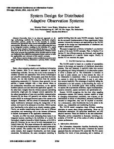
2.3 Direct vs Indirect Coding Based on the above explanations, the MT coding can be divided into two main categories of direct and indirect observations as depicted in Fig. 2.3. For the direct observations, the sensors are placed at the exact data locations such that their observation is complete. While, in indirect observation scenario, the observations are incomplete due to sensing error or physical distance between the source and observing data. Therefore, the proposed coding scheme aims at discovering the source by eliminating observation errors by means of employing many sensors. In MT coding, there are at least two observers and one or more sources. 2.4 Remote Sensing Remote sensing refers to sensor applications, where the sensor can not be placed at the exact data location, hence observation error is unavoidable. Remote sensing with a large number of potential applications has attracted a great deal of in the past decades. [55–57]. Remote sensing is modeled in different ways with the common unifying property of indirect observation meaning that one or several sources are monitored by one or several finite-accuracy remote observers. The objective is to reconstruct the source data with certain fidelity from the noisy observations gathered from sensors using the least possible description bits. A general model, which covers most cases is depicted in Fig. 2.3(a). If the observers are more than one, then this is equivalent to the problem of multi-terminal coding with indirect observations. 2.5 The Chief Executive Officer Problem The CEO problem can be viewed as the intersection of remote sensing and MT coding of indirect observations. In this case, there is only one source, but more than one indirect observers. The CEO problem has witnessed special attention in the past
16
𝑁1
𝑆1
𝑁𝑖
𝑆2 ⁞ 𝑆𝐾
⁞
+
𝑋1
Encoder 1
+
𝑋𝑖
Encoder i
⁞
⁞
𝑁𝑗 𝑁𝐿
+
𝑋𝑗
+
𝑋𝐿
Encoder j
𝑆̂1 (𝑡)
𝑅1 ⁞
𝑅𝑖
𝑆̂2 (𝑡)
⁞
Joint
𝑅𝑗
Decoder
⁞
⁞ Encoder L
⁞
𝑆̂𝐿 (𝑡)
𝑅𝐿
(a) direct observation
𝑋1 = 𝑆1 𝑋𝑖 = 𝑆𝑖
⁞
⁞
𝑋𝐿 = 𝑆𝐿
𝑆̂2 (𝑡)
𝑅𝑖
Encoder i ⁞
𝑋𝑗 = 𝑆𝑗
𝑆̂1 (𝑡)
𝑅1
Encoder 1
Encoder j
⁞
Joint
𝑅𝑗
Decoder
⁞
⁞
𝑅𝐿
Encoder L
⁞
𝑆̂𝐿 (𝑡)
(b) indirect observation
Figure 2.3: Multi-terminal source coding with direct and indirect observations.
17
years due to its more reasonable practical meaning in remote sensing, where multiple observers employed to compensate the observation imperfectness. The term CEO problem is borrowed from the context of business and economic studies and refers to a case, where the CEO of a firm is interested in collecting information about the firm by employing a team of agents. Each agent has partial observation and they are not permitted to confer and pool their data. The CEO aims at assigning enough number of agents and getting enough amount of information from each agent to obtain a certain level of fidelity about what is going on in the firm. This problem was first introduced for communication systems by Berger in his famous work [21]. This special case arises if the correlation among two transmit symbols X1 and X2 in Fig. 2.1 is due to observing a common source, S [21]. Note that correlation between S and X1 along with the correlation between S and X2 always results in correlation between X1 and X2 , but the reverse is not true in general. Therefore, the CEO problem is considered as an special case of multi-terminal coding. Another important distinction is that in the CEO problem, recovery of X1 and X2 is not primarily desired and we are interested in estimating the common source S with minimum distortion level. Therefore, the results obtained for MT coding is not applied to the CEO problem as they are. However, it is obvious that there is a strong connection between the two objectives in the CEO problem and MT coding. An important commonly used assumption in the CEO problem is that the agents observation errors are independent. A system model for the CEO problem is depicted in Fig. 2.4. We formally define the CEO problem for the purpose of this dissertation as follows. Let us assume that {S(t)}∞ t=1 is an i.i.d hidden source random process. This source is indirectly observed by L observers (e.g. sensors). The observation of sensors are denoted by {Xi (t)}∞ t=1 . To implement separate coding, agent i picks an observation vector of n symbols, Xin = [Xi (1), Xi (2), ..., Xi (n)]. Then, the agent employs (n)
an encoder fi
: X n → I2nRi to compress and map it to a codeword Cin . Here,
18
𝑋1 (𝑡)
Observation 𝑆(𝑡)
𝑋2 (t)
𝑋𝐿 (t)
Encoder 1 Encoder 2
Encoder L
𝑅1
𝑅2
Decoder
𝑅𝐿
𝑆̂(𝑡)
Figure 2.4: System model of the CEO problem. Im = {0, 1, 2, ...m − 1} is the set of positive integer values below m. The rate of encoder is defined as Ri =
|Ci | . n
The decoder receives all compressed codes and applies
the decoding function g (n) : I2nR1 × I2nR2 × .... × I2nRL → S n to provide an estimate of � (n) (n) (n) the source vector Sˆn = g (n) (C1n , C2n , ..., CLn ) = g (n) f1 (X1n ), f2 (X2n ), ..., fL (XLn ) . The average distortion is defined as :
D(n) =
� 1 � E d(X n , Xˆn ) n
(2.10)
A rate L-tuple RD = (R1 , R2 , ...RL ) with target distortion D is said to be achievable provided that there exist encoder and decoder functions with these rates that ensure D(n) ≤ D if n is chosen large enough. Each L-tuple rate is an achievable rate and the closure set of all such rates is called the rate region denoted by R∗ (D) = S RD (r1 , r2 , ..., rL ) . In some problem definitions, one may be interested in mini(r1 ,r2 ,...rL ) P mizing the sum rate, which is defined as R = Li=1 Ri , for a given target distortion D. Therefore, the sum-rate distortion function is studied rather than the achievable rate. Finding sum-rate distortion function is a simpler problem. The first information theoretic study on the CEO problem is conducted in [21]. In the limit, if the number of agents approach infinity (L → ∞) and the agents are allowed to share their observations, then they are able to remove their independent observation errors and provide an accurate estimate of the common source symbol,
19
S. The resulting distortion is limited by distortion rate function D(R). This means that for infinitely large number of agents, the observation error can be totally eliminated by joint coding and the resulting distortion is only due to the limited sum-rate. As a special case, if the sum-rate R exceeds the entropy of source H(S), the CEO decoder can fully recover the source symbol with arbitrary low distortion in common Shannon sense D(R) = 0, R > H(S). However, in most applications, the communication among agents is practically infeasible due to either technical limitations or cost considerations. Therefore, the CEO problem in the literature usually refers to the case of isolated agents, who do not communicate with one another unless explicitly specified otherwise. The first result for the CEO problem states that there is no finite sum-rate R for which even infinite number of agents can recover the common source losslessly with zero distortion [21]. However, it was shown that for an infinitely large number of agents, the distortion decays exponentially as sum-rate approaches infinity. One immediate interpretation of this result is that for the CEO problem, there is an advantage for sensors to convene and jointly encode their observations. This is an important contrast with the Slepian-Wolf problem, where there is no advantage for correlated agents to convene and the separate coding scheme yields the same results as joint coding. The intuitive reason is that in the Slepian-Wolf problem, one is interested in the observations of agent, while in the CEO problem, the primary interest is in estimating an indirectly observed common source. Thus, the communication among sensors may help smooth out the independent observation errors and always there is a penalty for preventing agent convention in the CEO problem. The sum-rate loss of the CEO problem, which is defined as the difference between the sum rate of distributed coding and joint coding is studied for Gaussian CEO problem in [58].
20
2.5.1 The Rate Distortion Region of the CEO problem Finding the exact rate distortion function for the CEO problem is a long lasting problem for decades. Despite promising progress in finding rate region and inner and outer bounds for some special cases, the exact problem is yet to be solved. The rate region for the CEO problem is characterized in [21, 59] as follows: • W1 → X1 → (S, X2 , W2 ) and W2 → X2 → (S, X2 , W1 ) are both Markov chains; • R1 ≥ I(X1 ; W1 |W2 ), R2 ≥ I(X2 ; W2 |W1 ), R1 + R2 ≥ I(X1 , X2 ; W1 , W2 ); ˆ ≤ D, where • There exist a function f : W1 × W2 → S such that E[d(S, S] Sˆ = f (W1 , W2 ). This is based on auxiliary random variables W1 and W2 that are jointly distributed with the common source variables S. In the above equation, S, W1 , W2 are support sets of S, W1 , W2 , respectively. The auxiliary RV Wi can be interpreted as a quantized version (or a description) of observation Xi . The core idea is to perform Gaussian quantization method on the observation bits and then apply Slepian-Wolf coding to the quantized observations [23]. The above characterization known as the Berger-Tung rate region, defines the corner points. The convex hull of rate region formed by connecting the corner points is achievable using sharing argument. This region is still the largest known rate-region for the CEO problem. This rate region is derived using the concept of random binning. The core idea of the random binning scheme is that the codewords at the encoder are divided into bins and the encoder transmits the bin id, which requires fewer bits compared to sending the codeword. The larger the number of codewords in each bin, the higher the compression rate. Upon receiving the bin indices from all the encoders, the decoder picks one codeword from each bin such that these codewords are jointly typical [60].
21
This is an achievable rate region, which is very complex to compute due to using the concept of auxiliary variables. Hence, for arbitrary source distribution, correlation model, and distortion measurement the computation is not feasible [20, 23, 61]. In [62], new upper and lower bounds on the rate region for a general CEO problem is found. 2.5.2 Quadratic Gaussian CEO Problem An special case of the CEO problem arises when an arbitrarily distributed source S is monitored by a cluster of L sensors whose observation errors Nk (t) are modeled as Additive White Gaussian Noise (AWGN). Therefore, Xk (t) = S(t) + Nk (t), k = 1, 2, .., L, where Nk (t) is an i.i.d Gaussian random process with zero mean elements of 2 . The distortion measure for this case is usually chosen as MSE: variance σN k n
D
(n)
� 1X � n �2 � 1 � E X (t) − Xˆn (t) . = E d(X n , Xˆn ) = n n t=1
(2.11)
This case is called Quadratic AWGN CEO problem. In [63], an upper bound is found on the rate distortion function of this scenario. However, the exact rate region even for this case is still unknown. An important special case of Quadratic AWGN CEO is Quadratic Gaussian CEO, where in addition to observation errors, the source itself is a random process 2 with i.i.d elements of Gaussian distributed with zero mean and variance σX . It was
shown in [63], that the Gaussian source is the worst case, hence the rate distortion function obtained for Quadratic Gaussian case can be used as an upper bound on the more general Quadratic AWGN CEO problem. In [64], the sum rate-distortion function for the case of infinite number of equal observation accuracy agents is found as in (2.12). This has confirmed the original conjecture about the rate-distortion asymptotic behavior was made by Berger et al in [22].
22
R(D) =
2 2 2 σN σX +1 + σX − 1] log ( ), [ 2 2σX D 2 D
(2.12)
where x+ = max(x, 0). In [65], rate region of Quadratic Gaussian CEO problem is fully characterized based on the idea of Gaussian quantization followed by Slepian-Wolf coding. This case is the most important special case of the CEO problem, whose rate region is completely known. However, this rate calculation due to its implicit maximization nature involves extensive search operation, which is not efficiently computable for a large number of sensors. Recently, a simple outer bound for the multi-terminal source coding problem is presented for the Quadratic Gaussian case, in terms of Hirschfeld-Gebelein-Renyi maximal correlation, which yields an efficiently computable explicit expression for the outer-bound of the sum rate function [61]. 2.5.3 Generalizations of the CEO Problem The CEO problem is generalized in several other aspects. In [66–68], the Quadratic Gaussian CEO problem is generalized to the case where a number of sources, instead of one source, are observed by L agents as depicted in Fig. 2.3(a). Another generalization is the case, where one sensor has direct access to the source and hence its observation is error free, as depicted in Fig. 2.5. Therefore, the goal is to decode one sensor’s observation X0 using other sensors’ observations as side information. This is called the many help one problem and is studied in [69]. The CEO problem can be generalized in the sense that the CEO is interested in estimating both common source data and observation with arbitrary fidelity. This is depicted in Fig. 2.6. If the maximum allowable distortions of observations reconstruction D1 , D2 approach infinity meaning that the CEO does not care about the observation itself, this problem reduces to the classical CEO problem. On the other hand, if the 23
Encoder:
Encoder: ̂
Decoder ⁞
̂
⁞
Encoder:
Figure 2.5: Many help one problem: one sensor observes the source directly and the rest of sensors observe indirectly. maximum allowable distortions of the common source observations reconstruction D3 approaches infinity, the problem is reduced to two-terminal direct observation case. The rate region for this general case is characterized in [60].
𝑆
𝑋1
Encoder 1
𝑋2
Encoder 2
𝑌1
𝑌2
Decoder 1
𝑋�1 ~𝐷1
Decoder 3
𝑋�3 ~𝐷3
Decoder 2
𝑋�2 ~𝐷2
Figure 2.6: Robust multi-terminal coding with multiple descriptions. Another extension considers Gaussian vector sources rather than Gaussian scalar sources. Hence, the observations are also Gaussian vectors jointly distributed with the 𝑌𝐿
common source vector. This case is called Quadratic Gaussian vector CEO problem. Several inner and outer bounds on the sum-rate distortion region of the Vector Gaussian CEO Problem are derived in the literature [13, 70–72].
24
2.5.4 Notes on the CEO Rate Distortion Function It is noted that the rate-distortion region and even the simpler version of sumrate-distortion function for the CEO problem are not known in general. The ratedistortion relation for finite number of sensors with unequal observation accuracy is only known for some special cases, the most important of which is the Quadratic Gaussian case, where both the source and the observation errors are independent Gaussian distributed random variables. Even, for this special case, the exact rate region function is too complex to evaluate for a large number of sensors. Therefore, it is very common to use the approximate rate-region derived using the Slepian-Wolf method in order to evaluate coding performance [38,73]. The Slepian-Wolf region is a contra-polymatroid with vertices [74]. This means that we can neglect the source of correlation among sensors, which is due to observing a common source and only emphasize on the inter-sensor correlations as will be discussed in chapters 3 and 4. 2.6 Distributed Coding In parallel with finding the rate region for lossless case and rate-distortion region for lossy MT coding, code design for correlated sources is intensively investigated in the literature in order to improve compression efficiency [2]. The core idea is simply to use other sensors observations as side information for decoding a particular sensor observation. The goal is to minimize description bits used in the encoder, such that the estimation of source codes from the compressed version yields zero or a bounded distortion in lossless and lossy coding case, respectively. 2.6.1 Joint Coding vs Distributed Coding It is a well known fact that if multiple sources are correlated and one may want to reconstruct them at a common destination using their compressed versions, joint coding always outperforms independent coding [75]. Moreover, it was shown that in some 25
Table 2.1: Joint probability mass function of two correlated symbols X1 and X2 . pX1 ,X2 (x1 , x2 ) A B C D E F G H
A
B
C
D
E
F
G
H
1/32 1/32 0 1/32 0 0 0 1/32 1/32 1/32 1/32 0 0 0 1/32 0 0 1/32 1/32 1/32 0 1/32 0 0 1/32 0 1/32 1/32 1/32 0 0 0 0 0 0 1/32 1/32 1/32 0 1/32 0 0 1/32 0 1/32 1/32 1/32 0 0 1/32 0 0 0 1/32 1/32 1/32 1/32 0 0 0 1/32 0 1/32 1/32
cases distributed coding achieves the same performance as joint coding [17, 75]. In independent coding, both coding and decoding are performed independently for each symbol. While, in joint coding and distributed coding, decoding is performed jointly at the receiver. The distinction between joint coding and distributed coding is that in joint coding, the encoders are permitted to communicate and share their information, while this is prohibited in distributed coding. We illustrate this with the following example. Let us assume one intends to compress two discrete-valued sources X1 and X2 .
The sources X1 and X2 are jointly distributed with probability mass func-
tion (pmf) in table 2.1.
The support set (alphabet) of both symbols are X =
{A, B, C, D, E, F, G, H}. The following facts are simply obtained from table 2.1: 1. Both symbols X1 and X2 are uniformly distributed, which can be simply verified by calculating marginal probabilities. Therefore, their entropy can be simply found as :
PX1 (x1 ) = P (X1 = x1 ) =
X
PX1 ,X2 (x1 , x2 ),
x2 ∈X
� ⇒PX1 (x1 ) = 1/8, similarly PX2 (x2 ) = 1/8 , for ∀x1 , x2 ∈ X X 1 ⇒H(Xi ) = − PXi (xi ) log2 PXi (xi ) = 8. . log2 8 = 3 bits 8 x ∈X i
26
(2.13)
2. Similarly, the conditional and joint entropy is calculated as follows:
H(X1 |X2 = x2 ) = −
X
P (X1 = x1 |X2 = x2 ) log2 P (X1 = x1 |X2 = x2 )
x1 ∈X
1 = 4. . log2 4 = 2 bits 4 X 1 ⇒H(X1 |X2 ) = PX2 (x2 )H(X1 |X2 = x2 ) = 8. .2 = 2 8 x ∈X 2
⇒H(X1 , X2 ) = H(X2 ) + H(X1 |X2 ) = 5 bits.
(2.14)
This can be justified simply. Once the realization of symbol X2 is obtained, there are only for possibilities for symbol X1 , hence it can be described with only log2 4 = 2 bits, therefore totally 5 is required to represent both symbols. If one is interested in sending the outcome (X1 , X2 ) to a common destination with minimum bit per transmission such that both symbols are recovered losslessly at destination, there are three possible ways. These approaches are depicted in Fig.2.7: Independent Coding: In independent coding, each symbol Xi , i = 1, 2 is compressed using an independent encoder function fi without considering the correlation between two symbols. Therefore, to realize lossless coding, the minimum rate of each encoders is limited with the source entropy function Ri ≤ H(Xi ), i = 1, 2. One possible mapping is shown in table 2.2, where Gray coding is used as encoder function. The symbol Xi is simply mapped to Yi = fi (Xi ). Therefore, the sum rate is simply R1 + R2 = H(X1 ) + H(X2 ) = 6 bits/transmission. At the decoder, each symbol is decoded independently using the corresponding received bits Yi . The correlation among sources are not considered anymore, which obviously is not efficient.
27
X1
X2
Encoder : f1
Encoder : f2
Y1
Decoder : g1
Y2
Decoder : g2
X 1
X 2
(a) independent coding
X1
X2
Encoder : f1
Encoder : f2
Y1
Joint Decoder : g
Y2
X 1, X 2
(b) joint coding
X1
X2
Encoder : f1
Encoder : f2
Y1
Joint Decoder : g
Y2
X 1, X 2
(c) distributed coding
Figure 2.7: Illustration of three coding methods including independent coding, joint coding and distributed coding.
28
Table 2.2: Implementation of encoder f1 using Gray coding. x1
A
B
C
D
E
F
G
H
pX1 (x1 )
1/8
1/8
1/8
1/8
1/8
1/8
1/8
1/8
y1 = f1 (x1 )
000
001
011
010
110
111
101
100
Table 2.3: Probability mass function of E and mapping of encoder f2 . E = X 1 ⊕ X2
000
001
010
100
pE (e)
1/4
1/4
1/4
1/4
Eb = f2 (E)
00
01
11
10
Joint Coding: Another possibility is using joint coding and benefiting from the correlation among sources and the fact that both sources share the same receiver. In this scenario, encoder f1 compresses the first symbol X1 using the bit mapping in table 2.2 to yield output codeword Y1 . This requires H(X1 ) = 3 bits per symbol. Then, encoder 2, maps symbol X2 using the same mapping rule to generate Y2 . Then, encoder 2 calculates the hamming distance between mapped versions of symbols Y1 and Y2 as E = Y1 ⊕ Y2 , where operation ⊕ is modulo-2 addition. Since, Y1 and Y2 differ at most in one bits, the symbol E can take only 4 options {000, 001, 010, 001} and can be compressed into two bits Eb as shown in table 2.3. The number of required bits is equal to H(X2 |X1 ) = 2. Encoder 2 sends these 2 bits. Hence, a total of H(X1 ) + H(X2 |X1 ) = H(X1 , X2 ) = 5 bits suffices to send both symbols. This is less than that of the independent coding, H(X1 ) + H(X2 ) = 6 bits. Notice that the joint entropy is always less than or equal to the sum entropy. The justification is that, the second encoder has access to the other symbol and can only decode their difference rather than its own symbol. Decoding algorithm is straightforward. The decoder, first decodes symbol X1 using the received corresponding 3 bits of Y1 according to mapping in table 2.2. Then, it calculates E using the two received bits of Eb . Finally, the symbol X2 is computed as
29
Table 2.4: Distributed Coding by binning symbol X2 into 4 bins. X2 Si = f2 (X2 )
(000,111)
(001,110)
(010,101)
(100,011)
00
01
11
10
X2 = X1 ⊕ E. Despite its optimum performance, the obvious drawback of joint coding is the inter-sensor communication requirements. Distributed Coding: An important criterion in distributed coding is that the sensors are not permitted to communicate with one another in contrast to joint coding. However, the encoders should be designed in a smart manner such that the correlation among sensors is utilized efficiently in the coding algorithm. One commonly used approach is the idea of binning. We provide the following solution based on the concept of binning to implement distributed coding for the aforementioned example. To enforce source coding, the same encoding function f1 as used in joint coding is applied to symbol X1 using mapping of table 2.2. However, the possible outcomes of symbol X2 are divided into 4 disjoint bins, each of which is assigned with a bin id Si . In the context of source coding, bin and bin id are also called Coset and Syndrome, respectively. This concept is presented in table 2.4. The symbols are grouped into bins such that the symbols inside each bin have the maximum Hamming distance of 3 bits. Therefore, each bin includes two symbol of toggled bits. Encoder function f2 , instead of sending the symbol index sends Si , the index of the bin for which the symbol belongs. The decoder, first determines the symbol X1 using 3 corresponding bits. Then, it identifies the bin to which the symbol X2 belongs, using bin index Si . There are two options for symbol X2 . The decoder chooses the one, which is closer to symbol X1 in Hamming distance sense. Since the Hamming distance between symbols X1 and X2 is at most 1 (according to the correlation model) and the two symbols in each bin are 3 bits far apart, there is always a unique solution. In this case, similar to joint coding, a total of
30
R1 + R2 = H(X1 , X2 ) = 5 bits suffices to compress both symbols with the additional advantage of eliminating inter-encoder communications. 2.6.2 Rate Region for Coding of Two Correlated Sources The rate region for the lossless coding of two correlated sources are depicted in Fig. 2.8. An important fact is that the above-mentioned achievable rate pair of � (R1 , R2 ) = H(X1 ), H(X2 |X1 ) for both joint and distributed coding is obtained by compressing symbol X1 up to its individual entropy and then compressing symbol X2 up to its conditional entropy H(X2 |X1 ) for a given symbol X1 . This rate represents a corner point, which is marked with A in Fig. 2.8. This method of compression is equivalent to the problem of source coding with side information available at the destination [26]. The other corner point of (R1 , R2 ) = � H(X1 |X2 ), H(X2 ) is obtainable in a similar way. The line connecting these two points are achievable simply by the time-sharing technique. If coding with rates corresponding to the first corner point is used in α, 0 ≤ α ≤ 1 portion of time and the second corner point is used for the rest of time, then the average rate becomes � (R1 , R2 ) = αH(X1 ) + α ¯ H(X1 |X2 ), αH(X2 ) + α ¯ H(X2 |X1 ) , which sweeps the line connecting the two corner points. Time sharing argument is a commonly used technique to prove achievability of coding rate regions [17, 75]. If a time-invariant coding technique is required and time sharing technique is not allowed, the line connecting the two corner points is still achievable but may require a more complex coding scheme. The justification of the other borders of R1 ≥ H(X1 |X2 ) and R2 ≥ H(X2 |X1 ) is obvious, since the decoder requires at least H(Xi |Xj ) bits to reconstruct the symbol Xi , even if the other symbol Xj is available at the destination, since spending more bits for symbol Xj does not compensate the bits required to recover Xi .
31
RX2
H(X2)
0
H(X1)
RX1
(a) independent coding
RX2 H(X1,X2) H(X2)
A
H(X2|X1)
0
H(X1|X2)
H(X1)
H(X1,X2)
RX1
(b) joint coding & distributed coding
Figure 2.8: Rate region for independent, joint and distributed coding.
32
2.7 Practical Distributed Coding Design In this section, practical code design for the CEO problem is discussed. The two important properties of sequentiality and robustness of the decoding algorithm are presented next. 2.7.1 Successive and Parallel Decoding The decoding algorithm is divided into two main categories of parallel and successive decoding in the sense of sequentiality. In parallel decoding, the algorithm first tries to reconstruct the observations of all sensors. Then, the observation of each sensor is used as the side information in decoding their counterparts in an iterative manner to enhance the estimation accuracy. Ultimately, the estimate of the common source is obtained by the purified estimates of all sensors. This is depicted in Fig. 2.9(a). Most of these codes are based on a class of codes which are primarily designed for channel coding as will be discussed later. In successive decoding, the codeword of the first sensor is decoded to obtain an initial estimate of the common source. Then, this primary estimate is used as side information to decode the observation of the second sensor. This refinance process continues up to the last sensor, which provides the final estimate of the common source. The idea of successive decoding is inspired by a class of CEO problem is called Serially Structured CEO problem or simply Serial CEO. In this setup, the agents are ordered and communicate in one-to-the next fashion through rate constrained links as depicted in Fig. 2.9. Each agent receives the observation of the previous agent, decodes it and combines it with its own observation and sends the result to the next agent. The last agent in the chain is the CEO, which receives the combined observations of all other agents. This can also be considered as a generalization of the noisy Wyner-Ziv problem, since each agent treats its own observation as side information to decode other sensor’s observations. This scenario naturally requires a successive decoding scheme. Serially 33
Decoder 1
Estimator
Decoder 2
(a) parallel decoding
S
X1
Sensor 1
Y1
X2
Sensor 2
XL Sensor L CEO
Y2
Y L = S
(b) successive decoding for serial CEO
Encoder 1
Decoder 1
Encoder 2
Decoder 1
Encoder j
Decoder 1
S
⁞
⁞
⁞
⁞
Encoder L
⁞
Decoder 1
(c) Successive decoding for general CEO problem
Figure 2.9: Parallel and successive decoding for the CEO problem.
34
structured CEO system setup is rarely used, since it suffers from a severe drawback of dependency on the inter-sensor communication links reliability. A failure in a single sensor breaks down the inter-sensor communication chain and causes the whole system to shut down. Successive decoding can be used for the classical CEO problem as well. The rate distortion function of successive decoding applied to the Quadratic Gaussian CEO problem with MSD distortion is found in [76] and a practical implementation of successive decoding is proposed in [77]. Successive decoding performs well for robust CEO systems with guaranteed sensor operation. However, it is not appropriate for dynamic situations, where the sensors are more likely to fail. Failure of couple of sensors causes the estimation error to propagate through successive decoding, which misleads the decoding algorithm and causes it to diverge. Moreover, as will be discussed later, these codes require a very robust channel coding stage to combat channel imperfectness. Another disadvantage of the successive decoding algorithm proposed in [77] is that, a priori information about sensors observation accuracies is required in order to perform the successive decoding algorithm in a descending accuracy order. This limits the use of this approach in practice. 2.7.2 Robustness to Sensor Failure In the context of distributed source coding, such as the Slepian-Wolf problem and its extensions, the emphasis is on the compression efficiency but the system robustness is ignored. A DSC scheme, which is optimal in the sense of compression efficiency can be very sensitive to the encoder failure, i.e., the performance of the whole system may degrade dramatically when one of the encoders is subject to a failure [60]. In contrast, in the Multiple Description (MD) problem, the encoders construct several descriptions of the source and send them separately through unreliable channels to the destination. The decoders at the destination intend to reconstruct the source given any
35
subset of the descriptions. Therefore, the emphasis is on the reliability and not the efficiency [78–83]. However, this is a centralized source coding problem, which requires inter-sensor communications and therefore is not applicable to to the DSC scenario [78]. The robustness issue of MT coding based on random binning is due to its nature. This arises from the fact that the bin index is sent rather than the codeword and other sensors bin indices are required to identify the correct codeword. Consequently, the decoding algorithm is very sensitive to other sensors operations. If the decoder only receives the data from one of the encoders, then it may not be able to recover the correct codeword since the decoder only gets a bin index from one encoder and there are many codewords in that bin. In general, we can improve the robustness of the DSC scheme by reducing the number of codewords in each bin, which is a way to trade compression efficiency for system robustness. This is essentially the main idea of the robust DSC scheme proposed in [60,84]. This improves the performance of syndrome-based coding by compromising the compression efficiency. However, since the issue is due to the nature of decoding algorithm, it still remains for noisy environments, particularly if some of the sensors fail or malfunction. In chapter 3, we propose a robust coding scheme with smooth performance degradation behavior in case of a sensor failure. 2.7.3 Structured Distributed Source Coding The core idea of distributed source coding is to group the source outcomes into bins and to send the syndromes as depicted in Fig. 2.10. In lossless source coding, the decoder determines the encapsulating bins from the received syndromes, then looks for a possible set of codewords inside these bins such that they present the maximum correlations [17]. In the lossy case, the decoder refines the estimation with the aim of side information to obtain minimum distortion [85]. A key issue is that one may require to pick an extremely large number of input symbols to approach the theoretical limits defined by the rate region borders. This
36
Figure 2.10: Source coding based on random binning and joint typicality. assumption along with the idea of random binning are the key ingredients needed to apply the concept of joint typicality. Random binning and extremely long input lengths are the commonly used assumptions to prove the achievability of rate regions by MT source coding [17, 75]. However, they are not practically feasible. This is in analogy to channel coding, where the optimal coding is achieved by employing infinitely large number of input symbols and using randomly generated code books with i.i.d Gaussian distributed elements [75] under the context of joint typicality and Asymptotic Equipartition Property (AEP). To be more specific, if the alphabet of symbol Xi is |Xi | and one applies source coding of rate Ri to a sequence of length n, then the number of input sequences, the number of bins and the number of codewords in each bin are |Xi |n , 2nRi , and
|Xi |n , 2nRi
respectively. As an example, for n = 1000, |Xi | = 2, Ri = 0.5 , the aforemen-
tioned numbers are 1.07×10301 , 3.27×10150 and 3.27×10150 . Consequently, an optimal decoding based on joint typicality involves an extensive search operation to decode a single sensor, which grows exponentially with the large number of sensors. Therefore, it may take an extremely long time to decode with currently available computation technologies. This prevents the use of optimal coding in the most real time applications. This justifies the extensive research efforts to develop structured codes with tractable decoding algorithms for DSC.
37
2.7.4 Syndrome Based Structured Codes The idea of employing structured binning concept and generating syndromes in a systematic manner to compress correlated sources was first proposed by Ramachandaran in [26]. They introduced a practical syndrome-base DSC for continuous-valued correlated symbols. They implemented the concept of binning in the scalar quantization stage by assigning several quantization intervals with distinguishable distances to each bin. Then, they used a trellis-based coset construction method. This fundamental idea was a ground for subsequent attempts to construct practical distributed coding schemes for both continuous-valued and discrete-valued sources. One drawback of this scheme is that it provides only asymmetric coding rates, since they converted the problem of coding two correlated sources into the problem of source coding with side information available at the destination. This means that one symbol is compressed independently, while the second symbol is compressed assuming the first symbol is losslessly available at the destination. This scheme does not provide symmetric coding rates, which are of more interest in Homogeneous sensor network design. To eliminate the problem of undesired asymmetric coding rate and realize any arbitrary coding rate, practical MT codes are designed for both direct and indirect observations in the framework of Slepian-Wolf coded quantization and Wyner-ziv coding by means of source splitting technique [86]. The second property of this scheme is that it includes modifications in quantization stage, hence is not applicable to discrete-valued and continuous-valued sources with standard quantization and digitization stages. Moreover, this scheme is not universal, since the quantization stage should be customized to a specific source distribution and correlation model.
38
2.8 Channel Coding Channel codes are designed for Forward Error Correction (FEC) purpose by eliminating transmission errors and recovering the transmit data stream from the received noisy symbols. A brief overview of the channel coding concept and the most popular channel codes are provided next. The optimal channel codes, in most cases including point-to-point communications, can be simply developed by generating random Gaussian code books, whose elements are i.i.d zero mean Gaussian distributed random variables. The codebook includes M rows of Gaussian vectors of length n. The codebook is revealed to both encoder and decoder. The encoder picks a message to transmit from m possible options randomly indexed from 1 to M . Then it chooses a row from Gaussian codebook whose row number is equal to the message index. The encoder sends the row as the message (code-word) to the destination. The decoder receives the noisy version of the codeword and simply looks for one out of k rows from the Gaussian codebook, which is jointly typical with the received codeword. The decoder reports error if no or more than one rows of the codebook is jointly typical with the received noisy code-word. Otherwise, the index of the only jointly typical row is declared as the transmit message index. This coding scheme is called random coding. In this scheme, n samples are transmitted to carry a single message. Since, the number of input messages are M , it can be described by k = log2 M bits. Therefore, the operational information rate is R(c) =
log2 M n
bit/channel use determines the maximum information bits that can be sent
error-free per channel use. It was shown by Shannon in his famous work that in order to ensure an error free transmission, the coding rate should be bounded by the Channel Capacity C, defined as the maximum mutual information between the input and output symbols I(X, Y ) for any specific channel determined by p(Y |X) [87]. For instance, the channel capacity of a point-to-point AWGN is specified as C = log2 (1 + 39
P ), N
which is called Shannon
Limit of AWGN channel with Signal to Noise Ratio of SN R =
P . N
The coding rate
R(c) can approach C in limit for extremely large input sequence, n → ∞. Achievable coding rate for more complex communication channels including Broadcast, Multiple Access, Relay, Z, and Diamond under input distributions, noise and interference models is throughly investigated in the literature [75]. Despite very simple and straightforward methodology of this coding, it has couple of disadvantages as follows. Although the variance of output codeword elements is constrained with the average transmit power, but the instantaneous amplitude of each element of the output codeword can be arbitrarily high due to the Gaussian distribution property, which renders this method impractical. Therefore, coding rate calculations are revisited, when the constraint is on the output codeword amplitude and not on the average expected power [88–90]. Another disadvantage of this scheme is that output codewords contain continuous-valued Gaussian distributed elements, which are not appropriately mapped into the existing modulation schemes with limited constellation points. Furthermore, very long frame lengths, which is an essential requirement in the operation of these codes, impose long delays on the transmission system. The last and the most important drawback is the computational complexity of decoding algorithm due to the need of extensive search operations and huge number of calculations involved in finding the jointly typical sets for extremely long frame lengths. This is similar to the impracticality argument of optimal source coding based on random binning concept. Consequently, these codes have not been used in practice and many research works during the past decades are devoted to find practically decodable channel codes with near-optimal error correction capabilities [91–93].
40
2.8.1 Practical Channel Codes Practical channel codes are developed for both binary and non-binary data streams [94–97]. However, we focus our attention on the binary channel codes throughout this dissertation. The basic operation of binary channel coding is that the encoder picks a data sequence of k bits and adds an additional parity bits to form the output sequence of n bits, where k < n. The ratio of input bits to output bits is called coding rate and denoted R(c) = k/n, which is usually less than one for equiprobable binary inputs in a point-to-point communication framework. The decoder receives the noisy versions of the output bits and recover the original input bits [98]. Such a code is represented by (k, n, e) or (k, n) in coding theory literature, where e presents the largest number of recoverable error bits. 2.8.2 Block Codes and Convolutional Codes Practical structured channel codes are divided into two main categories of block codes and convolutional codes. Other types of channel codes such as rateless erasure codes (fountain, Luby Transform (LT)1 , and Raptor codes), and polar codes have been recently developed with some special properties that are out of scope of this work. An encoder in a block code picks an input vector of a certain length, then multiplies it by a matrix, called Generator Matrix to produce an output codeword usually longer than the input sequence. The decoder multiplies the received noisy codeword with a parity check matrix to find the error vector. In case of error occurrence, usually Belief Propagation (BP) message passing algorithms are used to find the most likely transmitted bits. The most important variants of block codes are Hamming, Golay, Reed-Solomon (RS), BCH2 , Low Density Parity Check Codes (LDPC) and Low Density Generator Matrix Codes (LDGM) codes. 1 2
Invented by Luby Invented by Bose, Chaudhuri and Hocquenghem.
41
Convolutional codes, in contrast, are developed using finite state machines and are represented by trellis diagrams. Each output bit is generated as the linear combination of few precedent input bits (in non-recursive codes) or both input and output bits (in recursive codes). The operation is performed over Galois Field, GF(2) for binary inputs and is described by generating polynomials. Therefore, convolutional codes do not require long input frames and are appropriate for real time coding. Viterbi decoding, Soft Output Viterbi Algorithm (SOVA) and BCJR3 Maximum A Posteriori (MAP) are among the most popular decoding algorithm to decode convolutional codes. Serial and parallel combination of several convolutional encoders are called turbo codes, which are widely used due to their promising near Shannon-limit error recovery performances. It is notable that if a convolutional encoder of rate R(c) is applied to an input vector of finite length k, an output codeword of length k/R(c) is obtained. Thus, the inputoutput relation can also be represented by a generator matrix similar to block codes. In this work, convolutional codes are chosen as essential building blocks of the proposed coding scheme with details presented in chapter 3. 2.8.3 Source Coding Using Channel Codes As stated earlier, channel codes are designed for error recovery purposes. The objective in source coding is to remove the intrinsic redundant information from the input stream to perform compression, while in channel coding, an additional redundancy is added to the input data intentionally to facilitate error recovery. These two objectives seem contradictory. However, channel codes are widely used to perform distributed source coding as discussed in this section. The most popular channel codes used in DSC are LDPC and Turbo codes as follows. 3
Invented by Bahl, Cocke, Jelinek and Raviv.
42
2.8.3.1
Syndrome Based DSC Using LDPC Codes The use of LDPC codes to perform DSC is proposed in several papers includ-
ing [27, 99]. The authors considered compression of two correlated sources X1 and X2 . They first converted the problem to the equivalent of source coding with side information available at the destination. The symbol X1 is first compressed up to its entropy H(X1 ) with any traditional source coding technique such that it is fully reconstructed at the destination. Therefore, the problem was reduced to compress X2 up to its conditional entropy H(X2 |X1 ) such that it is fully recoverable by the decoder using X1 as side information. To solve this problem, LDPC codes are used in an innovative manner. Instead of employing generator matrix Gk×n of an LDPC code (k, n) with rate R at the encoder, the parity check matrix Hn−k×n is utilized. An input vector of length n is multiplied by H to result syndrome S2 of length k − n bit enabling compression of rate
k−n . n
For instance, an all zero syndrome of length n − k is obtained for all of the 2k possible n bit codewords of the corresponding LDPC codes. Likewise, each realization of 2n−k syndromes represents 2k input vector of length n. The decoder considers the syndrome S2 as the compressed version of X2 and the other symbol X1 as side information. The decoder treats the side information as the noisy version of the codeword and applies a classical belief propagation algorithm. The only difference is that in the message passing algorithm over the corresponding tanner graph, a negative sign is applied for any non-zero bit in the syndrome. In simple words, the side information X1 is used to initialize the tanner graph and the iterative belief propagation algorithm is performed using the compressed version of the source data S2 . This approach is depicted in Fig. 2.11. The message passing algorithm is modified such that the messages pass from the check nodes to the variable nodes change sign if the corresponding syndrome bit is 1. This approach performs very well but has a number of drawbacks: i) The codes are not capable of producing symmetric rates, since the operation is limited to the corner points of the Slepian-Wolf region; ii) The decoding algorithm is very sensitive to the 43
1
Uncompressed binary source output
0
0
1
1
0
0
1
0
Compressed output (syndrome)
1
Variable nodes
Check nodes
Figure 2.11: Using LDPC codes to implement syndrome-based distributed source coding. side information (error propagation issue). The second drawback is critical, since the decoding algorithm fails and the whole bits of syndrome become totally useless if the side information is lost. 2.8.3.2
Using LDPC Codes with Puncturing to Realize DSC To eliminate the above mentioned problems, another approach is proposed which
employs LDPC codes to enforce source coding [1, 100]. In this approach, a generator matrix of a systematic LDPC is employed at each encoder and a corresponding parity check matrix is employed at the decoder. Each encoder sends the resulting parity bits along with the part of systematic bits, such that all the encoders together form a complete set of systematic bits. Hence, compression is achieved by puncturing the systematic bits. The decoder performs a modified belief propagation algorithm considering the correlation model on a joint tanner graph representing all LDPC encoders embedded at sensors. A block diagram of this scheme is depicted in Fig 2.12. This approach has the advantage of i) providing arbitrary coding rates by tuning puncturing pattern, ii) eliminating error propagation phenomenon and sensitivity to the side information, and iii) simplicity of combining with the channel codes to implement distributed joint source channel coding as will be discussed in sequel. The main 44
X1 (k bits)
X2 (k bits)
Systematic LDPC Encoder (rate R1)
Systematic LDPC Encoder (rate R2)
Y1
Y2
αk
parity
(1-α)k
Decoder 1
parity
Decoder 1
Joint Decoder X1
X2
Figure 2.12: Using LDPC codes with puncturing to implement distributed source coding as proposed in [1]. drawback is degradation in compression efficiency with respect to the syndrome-based techniques. This method similar to the syndrome-based LDPC coding requires requires considerably big storage capacity and matrix operation capability at the encoder side, which might be difficult to implement in tiny sensors with limited computational power. Recently, LDGM coding scheme as a special class of LDPC coding with low density generator matrix is proposed to be used in distributed source coding. This reduces the computational load of the encoders with compromising the coding efficiency [31, 101]. 2.8.3.3
DSC Using Turbo Codes A Turbo encoder is composed of two ore more convolutional encoders which
are connected through interleavers. These codes are commonly used channel codes with very good minimum distance properties due to the use of interleaver. Moreover, they can be efficiently decoded using iterative decoding algorithms which results in a near-optimal coding performance [102–104] . 45
To eliminate the need of memory requirements and matrix operation at the sensors, turbo based encoders are proposed to implement DSC [15, 28, 29, 36, 105, 106]. In this approach, a turbo encoder is embedded at each sensor to enforce compression. Typically, the coding rate of turbo encoder used for channel coding is less than unity meaning that the resulting codeword is longer than the input vector. To enforce compression, when a turbo code is used for source coding purpose, the following methods are proposed in the literature: • Applying heavy puncturing prior to encoding, such that an small part of input bits is applied to the constituent convolutional encoders (Pre-puncturing) [107]. • Applying puncturing after encoding, such that all the input bits is applied to the constituent encoders, but the resulting codewords are punctured to realize desired coding rate (Post-puncturing) [108]. • Using high rate constituent convolutional encoders, such that the number of output bits of all constituent encoders is less than the number of input bits [28, 109]. These methods are shown in Fig. 2.13. The resulting compression efficiency is promising and the main drawbacks are decoding complexity and difficulty of scalability an arbitrary number of sensors. A novel coding structure with modified decoding algorithm is proposed in chapters 3 and 4 that eliminates these drawbacks without degradation of the performance. 2.9 Distributed Joint Source Channel Codes Distributed source coding is applied to correlated sources to squeeze the number of bits required to reconstruct the source symbols at the destination. This includes the reconstruction with zero error (in lossless case) or limited distortion (in lossy case). The (s)
compression rate of sensor i is denoted by Ri as the ratio of output compressed bits to the input bits. The basic presumption is that the communication channels from encoders 46
pre-punctureing
Conv. Encoder 1 R1= k/n1>2
pre-punctureing
Conv. Encoder 2 R2= k/n2>2
Interleaver
(a) pre-puncturing Conv. Encoder 1 R1= k/n1>2
post-punctureing
Conv. Encoder 2 R2= k/n2>2
post-punctureing
Interleaver
(b) post-puncturing
Conv. Encoder 1 R1= k/n1>2 Interleaver Conv. Encoder 2 R2= k/n2>2 (c) high code rate
Figure 2.13: Distributed source coding using turbo codes with different compression methods.
47
to the common destination are error-free. Hence, compression is the only source of estimation distortion. This is not the case in error prone wireless channels. Therefore, a reliable communication from sensors to the destination is required by means of employing strong enough channel codes. For instance, when the channels from encoder to the decoder are parallel Gaussian channels, a channel encoder should be utilized after DSC stage. The rate of channel encoder i should met the Shannon limit requirement of Ric ≥ log(1+Pi /Ni ), where Pi /N1 is the signal to noise ratio (SNR) of channel i. Based on the Shannon’s source channel separation theorem, there exist a single coding scheme (c)
with an effective coding rate of Ri =
Ri
(s) Ri
such that results the same end-to-end error
rate. In simple words, the two stages of source and channel coding can be combined into a single joint source channel coding with an equivalent overall performance [75, 110]. In-fact it has been shown that D-JSCC outperforms the case of separate source and channel coding, if the sources are correlated [111]. This is of great importance for practical applications, since it considerably simplifies both coding and decoding algorithms. In the next chapter, a novel coding scheme is proposed to realize D-JSCC for the binary CEO problem.
48
Chapter 3 DISTRIBUTED JOINT SOURCE-CHANNEL CODING FOR BINARY CEO PROBLEM
3.1 Introduction In this chapter, a distributed algorithm is proposed for joint compression and transmission of data inside a cluster of sensors with correlated observations. This realizes a many-to-one communication setup from a cluster of sensors to a data fusion center at the final destination. This scenario applies to small-scale networks, where all transmitters directly communicate with the base station, the so called collocated network. For large-scale networks, this communication is performed through multi-hop communications via intermediate relay nodes. In this chapter, the focus is on the single-cluster system model and the extension to the large-scale clustered networks is provided in chapter 5. Several models are proposed in the literature to model the observation accuracy of sensors for various data sources [112–119]. Most of these models are customized to a specific category of sources. For instance, the correlation among several temperature sensors are far different than the correlation among several video sensors observing a common object. In this research, a system model based on using a binary source with BSC virtual observation channels are adopted that can be used as an approximate model for a wide range of existing applications. This fact is justified in section 6.3. A D-JSCC scheme is proposed in section 3.4, which is based on employing simple convolutional encoders and pseudo-random interleavers at the sensors.
A
modified MTD is employed at the destination that outperforms the currently used MTD decoders as presented in section 3.5. Finally, an information theoretic analysis is provided in section 3.7 to find the optimum number of sensors at each cluster. The goal is to avoid adding extra sensors to the cluster if they do not considerably improve
49
the estimation accuracy. Before elaborating on the details of the system, the general notations used in this chapter throughout the end of this dissertation is provided next. 3.2 Preliminary Definitions The following notations are used in the current and the following chapters, unless explicitly specified otherwise. Capital letters are used for Continuous-Valued Random Variable (CRV) and Discrete-Valued Random Variable (DRV); lower case letters for the realization of RVs; and bold letters for vectors and matrices. Operation x¯ = 1−x is used to show bit flipping of a binary value x. Operation ⊕ is modulo-2 addition over field GF(2). Notations P (.) denotes the probability mass function (pmf) of a discrete-valued RVs. Likewise, f (x) and F (x) denote the probability distribution function (pdf) and cumulative probability distribution function (cpdf) of a discrete valued RV, respectively. R ∞ −t2 /2 √1 e dt are used to present and Q(x) = Also, exp(x) = ex , sgn(x) = |x| x 2π x exponential, sign, and error functions, respectively. H(X) is the entropy of RV X and I(X; Y ) denotes the bitwise mutual information between RVs X and Y . All log functions are base 2. A summary of notations for both variables and functions are provided in Tables 3.1 and 3.2.
50
Table 3.1: Variable definitions. Variable Description S S(t) s(t) N L sL S ui (t) uki ei (t) cki xki βi βij R(s) R(c) R(p) Ri (r) Ai (r) Di (r) Ei Iq λ Ti τi T Si Wi Di C
binary common source as a r.v common source at time t realization of common source at time t number of sensors in a cluster length of observation vector a vector of realizations of common source for time t = 0, 1, ..L − 1 alphabet (support set) of S observation of sensor i at time t observation vector of sensor i with length k observation error of sensor i at time t encoded observation vector of sensor i with length k, binary version encoded observation vector of sensor i with length k, BPSK modulated version observation error parameter (bit flipping probability) for sensor i bit flipping probability between sensor i and j source coding rate channel coding rate puncturing rate effective coding rate of sensor i Apriori LLR of constituent decoder i at iteration r Aposteriori (output) LLR of constituent decoder i at iteration r Extrinsic LLR of constituent decoder i at iteration r set of nonnegative integer values less than q: {0, 1, 2, ..., q − 1} symbol arrival rate arrival time of symbol i interarrival time between symbol i − 1 and i packetization time service time of packet i waiting time of packet i Delay of packet i channel capacity
51
Table 3.2: Function definitions. Function |x| ||x|| sgn(x) x¯ x ⊕ y, x ∗ y exp(x) erf (x) Q(x) pX (x) FX (x) fX (x), f (x) P (x), PX (x) H(X) H(X) H(X, Y ) H(X|Y )
Value p p|u1 | + ...|un |, x = (u1 , ..., un ) |u1 |2 + ...|un |2 |x| x
1−x x(1 − y) + (1 − x)y ex R x −t2 √2 e dt 0 π R ∞ −t2 /2 1 √ e dt 2π x P (X = x) P (X < x) ∂ F (x) ∂x X P (X P = x) − pX (x) log2 pX (x) − − −
x∈X R∞
fX (x) log2 fX (x)dx
x=−∞ P
pX,Y (x, y) log2 pX,Y (x|y)
x∈X P ,y∈Y
pX,Y (x, y) log2 pX|Y (x|y)
Description norm 1 (Taxicab norm) norm 2 (Euclidean norm) sign function bit flipping modulo-2 addition exponential function error function Q function probability function cpdf of CRVs pdf of CRVs pmf of CRVs entropy of DRVs entropy of CRVs joint entropy of DRVs entropy of DRVs
x∈X
I(X; Y ) f ∗ g(x)
H(X) − H(X|Y ) R∞ − f (t)g(x − t)dt
mutual Information function convolution
t=−∞
bxc α ¯ [x]+ [x]+
max{i : i ∈ [0, 1, 2, ..., ∞), i ≤ x} 1−α max(0, x) min(0, −x)
floor function complement of coefficient
3.3 System Model The system model includes a single data source S, which is surrounded by a cluster of N sensors as depicted in Fig. 3.1. The sensors encode their observations and collectively transmit it over independent AWGN channels to a fusion center located in a central base station. The goal is to provide an accurate estimate of the common data source with the smallest possible coding rates in order to save the total power consumption and bandwidth usage. More details are provided in the following sections. 52
Base Station: Data Fusion
1
N
2
Source Cluster of N Sensors
Figure 3.1: System model: a binary source is observed by a cluster of N sensors. Correlation model: In some applications, the observation accuracy is modeled by assuming that the source sample and the measurements of the sensors are jointly Gaussian distributed. This is based on the assumption that the source is a Gaussian Random Process (RP) and the observation error of sensors can be modeled with AWGN. These assumptions do not cover majority of applications. In reality, the source spans a wide variety of parameters to be measured including light, temperature, humidity, stress, pressure, etc. This results in a very diverse set of probability distribution functions. Moreover, the observation channels from the source to the sensors are not always limited to Gaussian channels. A binary source model with a virtual BSC channel is used in this dissertation, which covers a wide category of sources as follows. Binary source model applies to a class of WSN applications, where the sensors are employed to detect an event [120–124]. For instance, fire detectors which are utilized to trigger a fire alarm system or light-detectors that are used to turn on road lights at night times are simply modeled as binary data sources, where binary digits 0 and 1 refer to the occurrence or absence of a target event. A variety of application scenarios can be modeled using a 2-D or 3-D field measurements for event detection [125]. Not
53
any event is necessarily detected by the observer sensors. Likewise, the sensors may announce false alarms. Therefore, the binary observations are subject to error that can be simply described by the bit flipping probability. Consequently, a source data S and the sensor observation X can be considered as the input and output of a communication channel, which flips the binary digits with a certain probability β, namely BSC(β) as depicted in Fig.3.2. 1-β
0
0
β S
X
β 1
1-β
1
Figure 3.2: Binary symmetric channel with input S, output X, and crossover probability β. For an asymptotic analysis, this simple model can be used for discrete and continuous valued RVs in a broad sense. If s is the source data sample with an arbitrary probability function and u is the measurement of a sensor, then u is quantized and digitized to ud = [u1 u2 ...uq ], where q is the number of bits per symbol and ui ∈ {0, 1}. In a similar way, sd = [s1 s2 ...sq ] can be considered as the digitized version of the source data using the same quantization and digitization algorithms. The probability of bit flipping error in sensor i due to observation imperfectness, for any application is upper bounded by a parameter β, 0 ≤ β ≤ 1/2, where
β = max{P (si 6= ui )},
Iq = {0, 1, 2, ..., q − 1}.
i∈Iq
(3.1)
In practice, different schemes (such as Pulse-code modulation (PCM) quantization with A-Law and µ-Law companding for speech signals and Grey coding for digitization) are used to minimize the distortion caused by bit flipping [126–131]. Based
54
on the aforementioned justification, a binary data source observed through BSC channels is widely used as a general model to present the observation inaccuracy of sensors at least as an asymptotic analysis [15, 15, 29, 37, 132–134]. Noting the above justification, the binary source data frame s = {s(k)}Lk=1 , which is an independent and identically distributed (i.i.d) Bernoulli sequence of length L with p(s(k) = 0) = p(s(k) = 1) = 1/2 is considered. The observations of sensor i, denoted as ui = {ui (k)}Lk=1 , is modeled as a source data passed through a virtual BSC channel with crossover probability βi < 0.5. Thus, ui (k) = s(k) ⊕ ei (k), where ei (k) is the observation error signal with
� � P r ei (k) = 1 = 1 − P r ei (k) = 0 = βi .
(3.2)
Parameter βi is called observation error of sensor i, throughout this dissertation. Accordingly, β¯i = 1 − βi is called observation accuracy of sensor i. Hereafter, the observation error probability is assumed to be equal for all sensors, βi = β, ∀i ∈ IN = {1, 2, ..., N }. Otherwise, the worst case β = max{β1 , β2 , ..., βN } is chosen. For Discrete Memoryless Channel (DMC), with the assumption of independent sensor observation errors we have:
P (u1 , u2 , ..., uN |s) =
N Y
P (ui |s) =
i=1
N Y L Y
P (ui (k)|s(k))
(3.3)
i=1 k=1
The observations of two sensors are conditionally independent given source data values. This means that {ui (k) → s(k) → uj (k)} forms a Markov chain for any i and j. This results in a pairwise correlation between the observations of any sensor pair. The relevant pairwise crossover probability between sensors i and j is βi,j , which can be calculated using the Bayes’ theorem as follows:
55
P (ui = α, uj = α) 1 − βi,j =P (ui = α|uj = α) = P (uj = α) P P (ui = α, uj = α|s = m)P (s = m) m=0,1 P = P (uj = α|s = k)P (s = k) k=0,1 P P (ui = α|s = m)P (uj = α|s = m)P (s = m) m=0,1 P = P (uj = α|s = k)P (s = k) k=0,1
=
(1/2)[(1 − βi )(1 − βj ) + βi βj ] = 1 + 2βi βj − βi − βj , 1/2
= 1 + 2β 2 − 2β
(noting: βi = βj = β),
(3.4)
where we omit the time index for the sake of notification convenience. Similarly, we have:
βi,j = P (ui = α|uj = α ¯ ) = 2β − 2β 2 α ¯ = 1 − α , α = 0, 1.
(3.5)
For an small observation error, β → 0 , the approximation βi,j ≈ 2β can be used. This result may be justified with another intuitive approach. A BSC channel with an equiprobable input is bidirectional and we have P (X = x|Y = y) = P (Y = y|X = x). Therefore, the channel between any two sensors is the cascade of two consecutive BSC channels with parameters βi and βj that results in a BSC channel with parameter βi,j = βi ∗ βj = (1 − βi )βj + βi (1 − βj ) = βi + βj − 2βi βj ≈ βi + βj = 2β. This observation is used in decoder design presented in section 3.5.
56
3.4 Distributed Coding for Sensors with Correlated Data A low-complexity D-JSCC algorithm for a cluster of sensors equipped with RSC encoders is proposed. The coding algorithm supports both heterogeneous and homogeneous WSNs. The heterogeneous structure with three sensors provides a basic minimum configuration, while the homogeneous structure has the advantage of equivalent sensors. In this coding scheme, each sensor formats its observation bits into input frames of length L denoted by uLi = [ui (0), ui (1), ...ui (L)]. Then, it interleaves and encodes (c)
the input frame using an RSC encoder to generate the output codeword of length L/Ri , (c)
where Ri
is the constituent coding rate. The resulting output codeword is punc(p)
tured using a puncturing pattern of rate Ri
bL/Ri c
to result punctured codeword ci
=
(c)
[ci (0), ci (1), ...ci (bL/Ri c − 1)], where Ri = Ri /R(p) is the effective coding rate of sensor i. The operator bxc is the largest integer value not greater than x. The punctured codeword is modulated and sent to the common destination. 3.4.1 Random Interleaver Interleaving prior to encoding increases the minimum distance of the output codewords, which in turn reduces the error floor. To develop the pseudo random block interleavers, we followed a simple method of matrix permutation. In this method, a data frame of length m.n is filled in a table of size m × n, row by row; then the rows are randomly permuted. The resulting table is again permuted column-wise. Finally, data is read column by column. This shuffles the input bits randomly. The design is repeated independently for each sensor and is revealed to the decoder [135]. 3.4.2 RSC Encoders A RSC constituent encoder is embedded at each sensor. The block diagram of the utilized RSC encoder, which realizes a finite state machine is depicted in Fig.3.3. This encoder can be easily implemented using a simple hardware composed of a shift 57
register, memory unit and binary adders. Hence, it is appropriate for tiny sensors with limited resources. Systematic Bits +
Input Bits +
Delay
Delay
+
Parity Bits
Figure 3.3: Employed RSC encoder. Cosing rate is : R(c) = 12 . The code is represented by [1
f (D) ], g(D)
where D is delay operator and the feed-
forward and feedback polynomials are arbitrarily chosen as f (D) = 1 + D2 + D3 and g(D) = 1 + D + D3 , respectively. f (D) and g(D) are irreducible primitive polynomials widely used in covulotional-based code design [104]. The memory depth of the encoder is 3, hence two tails bits are added to the end of the input frame such that the encoder terminates in the all zero state. This is an important requirement for decoding algorithms, which sweep the code trellis in forward and backward directions. Hence, the exact coding rate of the encoder becomes 1 . 2
L , 2∗L+2
which is slightly less than
The performance of RSC encoders is relatively poor with respect to the one of turbo
encoders in a point-to-point transmission system. However, in a binary CEO setup, due to the correlation among sensors observations, they collectively form a turbo-like encoder. The resulting BER performance is comparable with the one achieved by a distributed turbo encoder at equivalent coding rates, as will be shown next. 3.4.3 Puncturing Method The coding rate of the employed RSC encoder is 12 meaning that one information bit u is mapped into two bits, one systematic bit u and one parity bit p. In heterogeneous setup with three sensors, to obtain an effective coding rate of Ri = 1, puncturing pattern is set to uu, pp and pp, as described in section 3.4.4. In homogeneous setup with two 58
sensors, the puncturing bits are set to up and pu. This means that only half of the systematic and half of the parity bits are sent to yield the coding rate of Ri = 1. If more than two encoders are employed, any puncturing pattern can be used to yield the desired effective coding rate per sensor. The only consideration has to be taken into account is that the output of all encoders collectively should include all of the systematic bits; otherwise, the performance significantly degrades. For instance, if three sensors are employed, the puncture codewords of the three sensors may include the systematic bits at positions 3n, 3n + 1 and 3n + 2, respectively. Finally, it should be noted that the tail bits do not participate in puncturing and are fully sent to destination in order to undertake the important role of terminating the RSC encoders to all zero state. The punctured codewords are modulated using an arbitrary constellation to form bL/f.Ri c
transmit symbols xi
= [xi (0), xi (1), ..., xi (bL/Ri c − 1)], where f is the modula-
tion order. Without loss of generality, we consider Binary Phase Shift Keying (BPSK) modulation with f = 1 in this work; hence xi (k) = 2ci (k) − 1. The output frames are transmitted through statistically independent AWGN channels to the destination. The received noisy frames at the destination are denoted by bL/Ri c
yi = {yi (k)}k=1
.
Parallel Gaussian channels are assumed throughout this paper that can be realized with Time Division Multiple Access (TDMA) or Frequency Division Multiple Access (FDMA). The more complex Code Division Multiple Access (CDMA) is not used, since it has been shown that for a Multiple Access (MA) channel with equal-power transmitters and AWGN noise, it does not provide additional gain over TDMA and FDMA. However, for non-equal power transmitters, CDMA-based codings are advantageous. The use of orthogonal transmission by means of TDMA and FDMA ensures statistical independence of the channels from the sensors to the common destination.
59
3.4.4 DSC for Heterogeneous Mode The heterogeneous system with minimum-configuration is realized using N = 3 sensors as depicted in Fig. 3.4(a). The interleaver block is shown by Πi in this figure. Sensor 1 AW
Mod Sensor 2
RSC
Mod
GN
AWGN Receiver
BS C
Sensor 3
П
RSC
AW G N
S
C BS BSC
Mod
(a) Minimum configuration Heterogeneous sensors
e1 + e2
s
+ eN +
u1 u2
uN
Π1
RSC
BPSK
x1 xn
Π2
RSC
BPSK
ΠN
RSC
BPSK
xN
z1 + z2
+ zN
+
y1 y2
Joint Source Channel Decoding
s
yN
Sensor Structure Data Fusion Center
(b) Homogeneous sensor
Figure 3.4: Distributed coding: D-PCCC scheme is used to estimate the binary data source, S observed by a cluster of N sensors. In this scenario, the first sensor transmits its observation bits without encoding so that the output stream of the first sensor contains only systematic bits c1 = [c1 (1), c1 (2), ..., c1 (L)] = [u1 (1), u1 (2), ..., u1 (L)]. No puncturing is applied. The second sensor encodes the data using an RSC encoder. The resulting frame is punctured with pattern pp to leave only parity bits c2 = [c2 (1), c2 (2), ..., c2 (K)] = [p1 (1), p1 (2), ..., p1 (K)]. Finally, the third sensor encodes its data with the same RSC encoder after interleaving it to form the output sequence containing a new parity sets c3 = [c3 (1), c3 (2), ..., c3 (K)] = [p2 (1), p2 (2), ..., p2 (K)]. Puncturing is not performed 60
for the third sensor either. The coding rate of each sensor is set to Ri = 1 and the redundancy is provided by the intrinsic correlation among sensors observations. The output frames of these three sensors altogether form a multi-frame similar to the output frame of a generic two-branch turbo encoder distributed among the three sensors. The only difference with the regular turbo encoder is that the two parity sets are generated from the corrupted versions of the systematic bits. This property will be considered in decoder design. 3.4.5 DSC for Homogeneous Modes The two drawbacks of the DSC coding for the heterogeneous configuration are the scalability issue and the property of fixed coding rate. The above configuration can be modified slightly to convert to a homogeneous configuration shown in Fig. 3.4(b), which is easily scalable. In this configuration, each sensor consists of a pseudo-random interleaver followed by a RSC encoder. The encoded frames contain both systematic and parity bit sets that can be punctured properly to achieve the desired coding rates at both symmetric and asymmetric. The only difference among sensors are the randomly generated pseudo-random interleavers that cause no problem in run-time decoding, since the map of interleavers to sensor ids are revealed to the decoder at design time. The output frame of sensor i is ci = [ci (1), ci (2), ..., ci (K.Ri )], where Ri = Rc /Rp is the effective coding rate of the ith sensor. To obtain a symmetric coding rate set, we simply set Ri = Rc for all sensor ∀i ∈ {1, 2, .., N }. 3.5 Decoder Structure The received frames in both heterogeneous and homogeneous modes include at least one set of systematic bits with one or more punctured parity sets. Neglecting the observation error of the sensors, this is analogous to the output codeword of a PCCC
61
encoder. Inspired by this fact, a MTD is employed at the destination to decode the input data sequence. A block diagram of the decoder is depicted in Fig. 3.5. P1
Π
I1
DEC1
П-1
D1
+
E1
La1
1-β Correlation Extraction
. . .
Σ
1-β
Π In
β
. . .
Pn
DECM
Lan
-
П-1 Dn
Apriori . Info . Calculation .
+
En
Figure 3.5: Modified MTD utilized at destination to decode the received frames. The received channel symbols y = [y1 , ..., yN ] are demultiplexed and unpunctured into the systematic and parity bits corresponding to the existing sensors yi = bL/Ri c
{yi (k)}k=1
= [ui (1), ui (2), ..., pi (1), pi (2), ....], i ∈ IN .
Then, each frame is passed to the corresponding constituent Soft Input Soft Output (SISO) decoder. The number of constituent decoders is equal to the number of parity bit sets. There two important classes of SISO decoders include MAP and SOVA. Both decoders are initialized using apriori estimates of the systematic bits, then perform decoding on the received noisy symbols to produce enhanced estimates of the systematic bits. Both decoders are based on finding the most likely inputs by sweeping the corresponding trellis diagram. The main difference is that a MAP-based decoder intends to find the most likely value for each transmit symbol, while the SOVA algorithm tries to find the most likely input frame. In other words, MAP minimizes the bit error probability in contrast to the SOVA, which minimizes the packet error probability. MAP algorithm is chosen for distributed coding, since the frames corresponding to different RSC encoders might differ by a few bits and word error is unavoidable. Moreover, 62
since the estimates of systematic bits are exchanged among the constituent decoders, MAP algorithm results in a higher performance. In this work, the BCJR Max-LogMAP algorithm is used as constituent decoders to decrease the decoding complexity by applying log(ex + ey ) ≈ max(x, y) approximation [136–138]. To perform decoding, in the first step, the Log Likelihood Ratios (LLRs) of the input bits are found from the corresponding received symbols to yield input LLRs for the constituent decoders. The input LLR of bit k for sensor i is denoted by Ai (k) and is defined as log2
P (ui (k)=1|yi ) , P (ui (k)=0|yi )
Es which for an AWGN channel with SNR= N can be 0
calculated as:
Ai (k) =
4 Es yi (k) if the corresponding bit exits after unpuncturing, N0 0
where
Es N0
(3.6)
else,
is the channel SNR. Then, A BCJR MAP Algorithm is performed by decoder
i on the received noisy versions of the parity bits to generate the output LLRs, Di . The details of BCJR algorithm can be found in [137, 139]. Then extrinsic LLRs are calculated as difference between the input and output LLRs, Ei (k) = Di (k) − Ai (k), which quantifies the amount of estimation improvement obtained by performing one round of decoding. Due to the high correlation among frames corresponding to constituent decoders, intuitively, an iterative algorithm may enhance the estimation of input bits in consecutive iterations. In order to exchange soft information among constituent decoders in a MTD decoders, there exist different structures including serial, master-slave, and parallel. Parallel structure is chosen in this work, due to its superior BER performance and fast convergence property [140, 141].
63
In a classical MTD, the input LLR for each encoder is simply calculated as the summation of extrinsic LLRs of the rest of constituent decoders at the previous iteration:
(r) Ai (k)
=
N X
(r−1)
Ej
(k),
(3.7)
j=1 j6=i
where postscript (r) denotes the iteration number. However, this does not applied to our case, where the extrinsic LLRs are corresponding to different sensor observations. Hereafter, the bit position index k is omitted for notation convenience. First, the same correlation model between the source and the observation bits are applied to the extrinsic LLRs of all decoders such that each provides a purified estimate of the common source data bits as follows: (r)
Es,i (n) = log2 = log2 = log2 = log2
p(s(n) = 1|ui ) � p(s(n) = 0|ui ) ˆ i (n) = 0|ui ) + (1 − β)p(u ˆ βp(u i (n) = 1|ui ) � ˆ ˆ (1 − β)p(u i (n) = 0|ui ) + βp(ui (n) = 1|ui ) ˆ p(ui (n)=1|ui ) � βˆ + (1 − β) ˆ + (1 − β)
p(ui (n)=0|ui ) i (n)=1|ui ) βˆ p(u p(ui (n)=0|ui )
ˆ Ei(r) (n) � βˆ + (1 − β)2 , ˆ + β2 ˆ Ei(r) (n) (1 − β)
(3.8)
where the extrinsic LLRs of each decoder at each iteration is scaled down with the observation error parameter βˆ to provide more accurate LLRs of the source bits. An algorithm to estimate the observation error parameter is presented in section 3.5.1. Then, the summation of these scaled extrinsic LLRs obtained from all constituent decoders except one is used to provide the input LLRs for that particular decoder as:
64
(r) Ai
=
N X
(r) Es,i
j=1 j6=i
=
N X
log
j=1 j6=i
(r−1) i h βˆ + (1 − β)2 ˆ Ej (r−1)
ˆ + β2 ˆ Ej (1 − β) (r−1)
= log
N ˆ ˆ Ej �Y β + (1 − β)2
(r−1) Ej
ˆ ˆ j=1 (1 − β) + β2
�
,
(3.9)
j6=i
The information exchange continues for a predefined number of iterations or until the decoding algorithm converges to an output sequence. At the last iteration, the estimates of the common source bits are obtained. First, the extrinsic LLRs are scaled based on the correlation parameter β, similar to the output LLRs modification in (3.8). Finally, Maximum Likelihood Detection (MLD) is applied to provide an estimate of the source data, sˆ(n) at the last iteration r = R. The MLD, for the case of equal-accuracy sensors is reduced to the sum operation followed by a hard limiter as follows: (R) Ds,i (n)
= log2
ˆ Di(R) (n) � βˆ + (1 − β)2 , ˆ + β2 ˆ Di(R) (n) (1 − β)
sˆ(n) = 0.5 1 + sgn
N X
�� (R) Ds,i (n) .
(3.10)
i=1
3.5.1 Correlation Extraction Method Since the observation error parameter, β is needed in the decoding algorithm, a two step algorithm is proposed to estimate β using the output LLRs. The estimation is performed at the end of the first iteration and is updated at the subsequent iterations as follows. At the end of each iteration, an estimate of transmit symbol xi (k) is found as xˆi (k) = sgn(Di (k)). This estimation tends to get closer to the transmit symbol after each iteration of decoding algorithm by canceling the noise effect. Therefore, we have
65
xˆi (k) ≈ 2xi (k) − 1 = 2[s(k) ⊕ ei (k)] − 1,
(3.11)
where the approximation improves over iterations. Theorem 3.5.1 If ρij is defined as ρij (k) =
|ˆ xi (k)−ˆ xj (k)| 2
for the estimates obtained from
the ith and ith sensors. Then, the following expression provides an estimate of the observation accuracy parameter, β with arbitrarily low estimation error given the frame length is chosen large enough L → ∞.
βˆ ≈
N −1 X L X 1 ρi,i+1 (k). 2L(N − 1) i=1 k=1
(3.12)
Proof Noting (3.11), ρij (k) defined above can be rewritten as:
ρij (k) =| [s(k) ⊕ ei (k)] − [s(k) ⊕ ej (k)] | .
(3.13)
It is easy to see that ρij (k) takes only two values of 0 and 1. If the bit flipping error occurs only in one of the sensors, then ρij (k) = 1. Therefore,
P (ρij (k) = 1) = P (ei (k) = 1) ∧ P (ej (k) = 0) + P (ei (k) = 0) ∧ P (ej (k) = 1) = (1 − βi )βj + βi (1 − βj ) = βi + βj − 2βi βj = βij = 2β(1 − β), (3.14) where the last equality is due to the equal observation error of sensors. However, the algorithm works for non-equal case as well. Expected value of ρij (k) is calculated using (3.14) as
E(ρij (k)) = 0.P (ρij (k) = 0) + 1.P (ρij (k) = 1) = βij .
66
(3.15)
Since ρij (k) is either 0 or 1, it immediately results that (ρij (k))2 = ρij (k). Moreover, the observation errors are independent over time. Therefore, we have:
E[(ρij (k))2 ] = E(ρij (k)) = βij ,
(3.16)
E[ρij (k)ρij (l)] = E(ρij (k))E(ρij (l)) = βij2 .
(3.17)
To obtain a higher accuracy, we take the time average of ρi,j (k) over the whole frame bits corresponding to two consecutive sensors. Then, we have: βˆi,i+1 =
PL
k=1
ρi,i+1 (k) L
(3.18)
with the following first and second order moments: L P
E(ρi,i+1 (k))
E(βˆi,i+1 ) =
k=1
2 E(βˆi,i+1 )=
1 E[ L2 k=1
L L L XX
= E[ρi,i+1 (k)] = βi,i+1 ,
(3.19)
ρi,i+1 (k)ρi,i+1 (l)]
l=1
L L L 1 X 1 XX 2 = 2 E[ρi,i+1 (k)ρi,i+1 (l)] E[(ρi,i+1 (k)) ] + 2 L k=1 L k=1 l=1 l6=k
1 L(L − 1) (βi,i+1 ) + (βi,i+1 )2 L L2 1 2 2 ⇒ σβ2ˆi,i+1 = E(βˆi,i+1 ). ) − E 2 (βˆi,i+1 ) = (βi,i+1 − βi,i+1 L =
(3.20) (3.21)
2 Therefore, βˆi,i+1 is a RV with mean βi,i+1 and variance L1 (βi,i+1 − βi,i+1 ). The
variance approaches zero if the frame length L is selected large enough. Thus, βˆi,i+1 provides a good estimate of the inter-sensor crossover probability. The sensor observation error parameter is estimated as βˆ ≈
βˆi,i+1 2
noting (3.5). In order to remove
the dependency of the estimation accuracy on a particular sensor pair, the inter-sensor crossover probability is averaged over all N − 1 consecutive sensor pairs as
67
βˆ ≈
N −1 X 1 βˆi,i+1 , 2(N − 1) i=1
which further improves the estimation accuracy by lowering the variance.
(3.22)
This
completes the proof. The simulation results presented in section 3.6 verify the accuracy of this method such that no considerable BER performance is noticed for the decoder with this selfobservation estimation block with respect to a system with known observation accuracy at the destination. 3.5.2 Summary of Modifications to Decoding Algorithm The following are a list of modification made to the MTD decoder, most of which are based on the fact that the parity bits are generated by different sensors from corrupted versions of the common data source: • Decoder Initialization phase: In a classic MTD decoder, since all parity bit sets are corresponding to the same systematic bit set, the LLRs of the systematic bits are applied to one RSC decoder at the initialization phase. While, each RSC decoder in the proposed system model corresponds to a particular sensor with a particular observation bit set. If one systematic bit set is available, which is the case in heterogeneous mode, the LLRs of systematic bits are fed into the all RSC decoders rather than a particular RSC decoder in the initialization phase. In homogeneous mode, the systematic bits of each sensor are applied to the corresponding RSC decoder. • LLR exchange: The input LLR for each decoder is calculated as the average over the output LLRs of the all other RSC decoders. The inter-sensor crossover probability stated in section 6.3 is taken into account in this process. The extrinsic LLRs 68
of each decoder is scaled down based on the correlation model before applying as a-priori information to the other decoders. • Decision phase: In the last iteration, hard decision is performed on the average P of output LLRs, D(av) = N1 N i=1 Di instead of the output LLR of a particular RSC decoder, for the similar reason. This yields a better estimate of the common source data, since each decoder intends to converge to the corresponding sensor’s observation bits that might be slightly different than common data source. Moreover, the output LLRs are adjusted based on the corresponding sensor observation accuracy parameter before participating in the final estimation process. • Observation accuracy estimation: As detailed in section 3.5.1, accurate estimates of the sensors observation accuracies are made using the received data. 3.6 Performance Analysis In order to demonstrate the BER performance improvement through the modifications applied to the MTD decoder, the operation of this decoder is analyzed using Monte Carlo simulations. The three-sensor heterogeneous system is compared to a N P standard two-branch turbo decoder with the equal sum code rate, R = 1/ R1i . The i=1
simulation parameters include i) data frame length: 256 bits, ii) data source distribution: equiprobable binary Bernoulli sequence, iii) modulation: BPSK, iv) observation error: β = 0.01, v) coding rate per sensor: Ri = 1 (since each sensor transmits either systematic bits or parity bits). It is apparent from Fig. 3.6 that the modified decoder, represented by ’ModifiedTC’ outperforms the standard decoder shown by ’TC’ in this figure. The BER floor of the proposed scheme is in the order of 10−3 , while the minimum achievable BER floor using a standard turbo decoder is in the order of 10−2 . ’Modified-MTC’ represents the homogeneous system composed of three sensors operating at coding rate R =
69
1 2
that
shows higher BER performance and lower BER floor at the same SNR levels. This improvement is trivial and achieved at the cost of lower channel coding rate or correspondingly higher bandwidth usage. 0
10
TC (N:3, Rate = 1) Modified−TC (N:3, Rate = 1) Modified−MTC (N:3, Rate = 1/2)
−1
BER
10
−2
10
−3
10
−4
10 −10
−8
−6
−4
−2
0 2 Es/No (dB)
4
6
8
10
Figure 3.6: Comparison of different decoding schemes for 3 sensors with correlated data (β = 0.01). Fig. 3.7 demonstrates the effect of the correlation parameter estimation in the proposed method. In the first method, the correlation parameter is assumed to be known at the receiver, while in the second method, it is estimated by post processing of the received symbols. Simulation results prove the accuracy of the developed estimation method, since the system BER performance for two cases are almost the same and there is no considerable BER performance degradation due to the estimation of correlation parameter at the receiver. 3.7 Optimum Number of Sensors In the previous sections, the performance of the proposed coding scheme was analyzed for a given situation including a predefined number of sensors. Obviously, using more sensors at each cluster would reduce the estimation error.
70
N=8 (Known β at decoder) N=8 (Self−estimation method) N=64 (Known β at decoder) N=64 (Self−estimation method)
−1
10
BER
−2
10
−3
10
−4
10 −20
−15
−10
−5
0
5
Es/N0
Figure 3.7: Comparison of BER performance of the modified MTD with known and self-estimated observation error parameters (β = 0.05). One may need to add more sensors to compensate the low observation accuracy of sensors in order to achieve higher estimation fidelity, as depicted in Fig. 3.8. At a specific point, the relation between the performance and the number of sensors saturates; hence the performance improvement is negligible by further adding sensors. Adding more than the required number of sensors to a cluster increases the decoding complexity, implementation and maintenance costs, power consumption and bandwidth usage without a considerable improvement in the estimation reliability. Therefore, an important question is how many sensors are required to achieve a desired BER level for a given observation accuracy and channel quality? The answer to this question is very challenging, since the rate distortion for a binary CEO problem with finite number of sensors is not known. Recently, a numerical based rate-distortion function is derived for the binary CEO problem in a noiseless environment that is computable only for two sensors [142]. The loss measurement is based logarithmic distribution distances. The rate calculations is by brute-force search over a
71
0
10
−1
10
−2
BER
10
−3
10
N:2 N: 4 N: 16 N: 32 N: 64 N: 128 N: 8
−4
10
0
0.05
0.1
0.15
0.2
0.25
0.3
0.35
0.4
0.45
0.5
Observation Crossover Parameter: (β)
Figure 3.8: BER performance of modified MTD vs BSC crossover probability for different number of sensors at SN R = −6 dB. fine mesh of conditional distributions. This rate is depicted in Fig. 3.9. This method can not be used for a large number of sensors in the presence of noise. To solve this paradigm in sensor networks, we consider a binary CEO problem in a cluster with equal and small observation error parameters. An approximate method based on the channel capacity concept is proposed to find the optimum number of sensors. First, we note that the best achievable BER is defined by the number of sensors regardless of the coding efficiency used to compensate the noise effect. Therefore, the BER floor is fully defined by the number of sensors in an error-free environment. The error floor for the case of equal-accuracy sensors is the probability of having correct observations at least by half of the sensors. For an even number of sensors, if exactly half of the bits are in error, the estimated bit can be arbitrarily set to 0. Hence, the following error floor becomes:
72
Figure 3.9: The rate distortion function for a binary CEO problem with two sensors and logarithmic loss measure.
p(min) error =
N � � X N β k + (1 − β)N −k , k N +1 k=
N is odd,
2
� � � � N X N N 1 N/2 N/2 β (1 − β) + [β(1 − β)]N −k , N is even k 2 N/2 N k=
2
+1
(3.23) In order to find the minimum number of sensors that ensure this error probability, a virtual communications from the source to the destination through cluster of N sensors is considered. If one find the capacity of such a channel, based on the Shannon theorem, one may utilize an encoder with coding rate less than or equal to the capacity such that the resulting error probability becomes arbitrarily small. However, in reality the coding is performed at the sensor nodes and not at the source node. However, we conjecture that if a encoder with coding rate below the found capacity is employed by the sensors, the resulting system will achieve almost the minimum BER defined by error floor in (4.20). 73
This conjecture is the core idea of the proposed analysis, which is well confirmed by the simulation results as follow in sequel. The methodology is to find a closed form expression for the end-to-end channel capacity that relates the system information capacity to the number of sensors and other system quality factors. Therefore, finding the channel capacity determines the maximum achievable coding rate for a given number of sensors, in a particular system setup. On the other hand, if the coding rate is fixed, the minimum number of sensors is determined to ensure a reliable communication system. Parallel AWGN Channel
BSC Broadcast Channels
z1 x1
+ z2
s
x2
+ zN
xN
+
y1 y2
s
Joint Decoder yN
Figure 3.10: Communication channel from source to destination: Cascade of BSC broadcast channels and parallel Gaussian channels. The virtual channel between the source and destination, as depicted in Fig. 3.10, is the cascade of broadcast BSC channels and parallel AWGN channels. In this section, S and Sˆ represent the source symbol and its estimate. The RV sets XN = {X1 , X2 , ..., XN } and YN = [Y1 , Y2 , ..., YN ] denote the sensors’ BPSK modulated observation set and the corresponding received symbols, with support sets χN and Y N , respectively. The following theorem holds for the channel capacity. Theorem 3.7.1 The capacity of a hybrid channel composed of a broadcast BSC(β) channels cascaded with N parallel Gaussian channels with SN R =
74
P σ2
is:
Capacity (Bit / Transmission)
1 0.8 0.6 0.4 0.2 10 0 0.5
5 0.4
0.3
0 0.2
0.1
Crossover Probability
−5 0
−10
SNR (dB)
Figure 3.11: Information capacity of system vs observation accuracy (BSC crossover probability) and channel quality (SNR) for 4 sensors.
Z
γ0 + γ1 ) − γ0 log(γ0 ) − γ1 log(γ1 )]dy N (3.24) 2 Yn k N √ 2 √ 2 P P (y − (2α − 1) (y + (2α − 1) P ) + P) � � � i i N � X N i=0 i=k+1 k (N −k) γα = β (1 − β) exp − 2 k 2σN k=0
1 C= 2 N/2 2(2πσN )
[(γ0 + γ1 )log(
Proof See appendix A.5. The information capacity in (3.24) is defined as a function of the number of sensors N , observation crossover probability β and the equivalent SNR at the receiver SNR =
P 2 . σN
Hence, it can be written as C = f (N, SNR, β). The obtained capacity curve
is depicted in Fig. 3.11. This figure shows that the capacity is directly proportional to the observation accuracy and to the channel quality as was expected. Figs. 3.12(a) and 3.12(b) provide two different slices of Fig. 3.11 to demonstrate the effect of observation accuracy and channel quality on the capacity curve more clearly.
75
Fig. 3.12(a) shows that the capacity changes considerably with observation accuracy. As an extreme case of totally unobservable source, when the BSC crossover probability is β = 21 , no information is exchanged regardless of the number of sensors and the sensor-destination channel quality. 1 N:1 N:2 N:3 N:4
0.9
Capacity (Bit / Transmission)
0.8 0.7 0.6 0.5 0.4 0.3 0.2 0.1 0 0
0.05
0.1
0.15
0.2 0.25 0.3 0.35 Crossover Probability
0.4
0.45
0.5
(a) C vs β, SNR = 0 dB. 1 0.9
Capacity (Bit / Transmission)
0.8 0.7
N:1 N:2 N:3 N:4 N:5
0.6 0.5 0.4 SNR = 0.578
0.3
SNR = −2.570 SNR = −4.366
0.2
SNR = −5.628 SNR = −6.621
0.1 0 −20
−15
−10
−5 SNR (dB)
0
5
10
(b) C vs SNR, β = 0.01.
Figure 3.12: Information capacity of system vs observation accuracy (BSC crossover probability) and channel quality (SNR) for 4 sensors.
76
In Fig. 3.12(b), the channel capacity is plotted for a fixed observation error parameter β = 0.01. The capacity is an increasing function of the channel SNR. If a certain value of capacity is desired, the minimum required SNR level is less for a higher number of utilized sensors. For instance, to achieve a capacity of
1 2
bit/transmission, the
required SNR values for N = 2, 3, 4, 5 sensors are −2.570 dB, −4.366 dB, −5.628 dB, and −6.621 dB, respectively. In another interpretation, for power constrained sensors (limited SNRs), this graph can be used to determine the minimum number of sensors to achieve a certain level of capacity. For instance, at least 4 sensors are needed to achieve a capacity of
1 2
bits/transmission at SNR = −5 dB. However, we note that the capacity
curve saturates at high SNR values and the maximum capacity is imposed by the number of sensors. Fig. 3.13(a) depicts the BER performance of the proposed coding scheme using Monte Carlo simulations. The observation error parameter is set to β = 0.01, data frames are 256 bit long, the RSC encoders operate at coding rate Ri = 12 , and the BPSK modulation is used as before. The results show that as the number of sensors at each cluster increases, the system end-to-end BER is improved at the cost of higher receiver complexity. Based on the Shannon’s theorem they achieve arbitrary low error rates at the SNR values higher than the limits derived from the capacity curves. The results confirm the sub optimality of the proposed coding scheme, since it achieves relatively low bit error rate at the SNR limits from channel capacity curves in Fig. 3.13(b). However, it is noticeable that the error floor can not be improved considerably by increasing the SNR value, since it is limited by the number of sensors and the observation accuracy. This is due to the fact that encoding is performed at the sensors and not at the source; hence, the information capacity between the source and sensors are limited. To achieve lower error floors for a certain β, a larger number of sensors must be employed at each cluster.
77
0
10
N=5 N=4 N=3
N: 2 N: 3 N: 4 N: 5 N: 8 N: 16 N: 64
N=2
SNR Limits −1
10
−2
BER
10
−3
10
−4
10
−5
10 −15
−10
−5 SNR (dB)
0
5
(a) Decoder BER Performance 1 0.9
Capacity (Bit / Transmission)
0.8 0.7
N:1 N:2 N:3 N:4 N:5
0.6 0.5 0.4 SNR = 0.578
0.3
SNR = −2.570 SNR = −4.366
0.2
SNR = −5.628 SNR = −6.621
0.1 0 −20
−15
−10
−5 SNR (dB)
0
5
10
(b) Capacity vs SNR, β = 0.01.
Figure 3.13: Analysis and simulation results for the impact of the number of sensors on the BER Performance (β = 0.01).
3.8 Summary of Contributions In this chapter, a binary CEO model with virtual BSC channels are studied to model a binary source monitored by a cluster of sensors for remote sensing applications. The extension of the model to cover the more general case of continuous and discrete valued sources with an arbitrary observation error is provided as an asymptotic analysis 78
model. A novel distributed coding technique based on PCCC is proposed that is the less complexity coding scheme reported so far to the best of our knowledge. The encoder in the proposed coding scheme requires very limited operations and a very small memory, hence is implementable in WSN with low-capability sensors. The complexity of the decoding algorithm grows linearly with the number of sensors and the decoding scheme is robust to sensor failures. This facilitates the scalability of the proposed scheme to any number of sensors. No prior information is required at the decoder about the sensors observation accuracies, hence it is extracted from the received data and is refined in an iterative manner. Therefore, the system tracks the observation accuracy parameter and adjusts the decoding algorithm accordingly [143]. Furthermore, an approximate information theoretic analysis is provided to relate the end-to-end information capacity to the channel conditions, sensor observation accuracies and the number of sensors. Therefore, for a fixed coding rate, the minimum number of sensors are found for a given system conditions. This can be used as an additional criterion to incorporate data flow efficiency to the currently available clustering algorithms [144].
79
Chapter 4 CONVERGENCE ANALYSIS
4.1 Introduction The use of channel codes to implement D-JSCC for correlated sources has been dominantly replacing the classical design of syndrome-based distributed source coding followed by a channel coding stage. In chapter 3, a novel implementation of D-JSCC is provided for the binary CEO problem, which realizes a distributed version of PCCC among sensors. This structure, intuitively requires a MTD-based decoder, which provides purified estimates of the common source data stream in an iterative manner. The decoder design is modified according to the utilized observation model, which presents a promising improvement to the system end-to-end BER performance. The use of iterative decoding is prevalent, when channel codes are used to perform both tasks of compression and error recovery in a noisy environment. A brief overview of these methods are provided in chapter 3 and more details can be found in the literature [2, 18, 32, 33, 35, 36, 38, 111, 145–150]. The core idea in the majority of these works is to benefit from the correlation among codewords generated by different sensors with the aim of iterative decoding. Analytical performance evaluations and simulation results suggest that the iterative decoding is the superior method to decode correlated sources in most cases. However, this question remains unanswered. Is the iterative decoding always optimal? If no, under what conditions the iterative decoding improves the estimation accuracy. In fact, a comprehensive literature review reveals that the uselessness of the extrinsic information exchange in iterative decoding for a number of situations have been noticed by former researchers. The following are three examples, where the iterative extrinsic information exchange is avoided due to its harmful effect on the decoding performance.
80
• In [107], turbo encoders have been utilized at sensor level to compress correlated binary data streams. Each embedded encoder in a sensor consists of two RSC encoders in parallel, which are connected via an interleaver. To achieve compression, the input bits are down-sampled prior to RSC encoding. Therefore, parity bits of each RSC encoder are formed by encoding part of the input bits. At the receiver, an iterative decoding is realized by exchanging the LLRs of input bits among two cooperative turbo decoders. However, the authors observed that participating the LLRs of all input bits may deteriorate the decoding algorithm. Therefore, they limit the use of extrinsic information exchange only to the common symbols of the two codewords. Although, both parity bit sets correspond to the part of the same observation bits, the exchange of LLRs corresponding to distinct part of the input bits is not useful anymore. This is similar to our proposed system model in the sense that for a low observation accuracy, the observation bits may be too different at different sensors, which make the parity bits far apart. Hence, the iterative information exchange becomes destructive rather than being constructive. • In [108], LDPC codes have been utilized to compress correlated binary sources, where the authors recognized that in some cases, the extrinsic information is not reliable initially and therefore is clipped at the first few iterations. This observation also confirms that the usefulness of iterative information exchange should be carefully examined. • The destructive effect of the iterative information exchange is noticed in [106], when the parity bits are produced using interleaved versions of different observation bit sets. In order to solve this issue, the interleaver block is placed after encoding to avoid harmful information exchange by generating consistent parity
81
bits. This unusual use of interleaver is not optimal and decreases the minimum distance of the resulting codewords, specially for short frame lengths. We conjecture that this effect was not seen in some other works, since they only have used very high accuracy sensors (β = 0.01, 0.001) in their simulations. It is notable, that this destructive effect does not occur in point-to-point communications, since the output codewords represent the same input data or interleaved versions of it. Therefore, the soft information exchange among the constituent decoders is always beneficial. These observations demand for a comprehensive study and careful analysis of the superiority of iterative decoding, when it applies to correlated sources. To the best of our knowledge, such a study has not been conducted, even for a specific case. In this chapter, we analyze this issue and characterize the situations, where the iterative decoder converges and outperforms the non-iterative one. This region, which is called Convergence Region in this dissertation, is specified in terms of the average channel quality (SNR) and the sensors observation accuracies (β). 4.2 Analysis Framework In order to develop an analysis framework to study the convergence of the proposed MTD decoder, let us review the decoding algorithm for two sensors. A simplified block diagram of the encoder/decoder pair is depicted in Fig. 4.1. As elaborated in chapter 3, each encoder observes a noisy version of the common binary data stream, encodes and transmits it to a common decoder. The decoder employs two constituent decoders to decode the observations of the two sensors and yield estimates of the corresponding observation bits. Due to the high correlation between the two sensors and the common source, the resulting estimates of each constituent decoder can be used by its counterpart to refine its own estimation in an iterative manner. This is the core idea of the proposed iterative decoding.
82
u1
x1
z1 +
Se n sor #1
y2
A1
SISO DEC 1
P1
D1 P2
E1 Final Estimation
S
A2
z2 u 2 S e nsor #2 x 2
SISO DEC 2
+ y 1
S
E2 D2
Figure 4.1: Simplified block diagram of the proposed encoder/decoder structure for two sensors. The objective of the proposed analysis in this chapter is to examine whether or not the output estimates of each constituent decoder get closer to the common source data bits. The two comparison points are marked with P1 and P2 in Fig. 4.1. This is substantially different from the commonly used techniques to analyze the convergence of a classical MTD, in the sense that the common data source are not necessarily the same as the observation bits used in encoding process. To be more specific, there might be a case, in which the output LLRs provide more accurate estimates of the observation bits than that of the input LLRs, but at the same time they diverge from the common source data bits. In such a case, the output LLRs of this decoder is not useful for its counterpart since they are misleading. This is the main distinction with the classic analysis of the iterative decoding. Therefore, we are interested in identifying the cases, where the soft information exchange among constituent decoders causes both decoders to yield a better estimates of the common source data bits. Since, this is the ultimate objective of the decoding process. 4.2.1 Modified EXIT Charts Analysis One commonly used technique to analyze the convergence property of iterative decoders is using EXIT charts. This methodology is used to examine how an estimation of a common source is improved by exchanging soft information among cooperative SISO decoders. The closeness of the estimated values to the target data can be measure
83
using different distance metrics, which results in developing different EXIT chart methods. Two important variants of EXIT charts are developed based on the LLR SNR and mutual information analysis [151, 152]. The LLRSN R value determines the accuracy of LLR and is defined as the mean over standard deviation for Gaussian distributed LLRs. In this work, we choose the mutual information-based method, proposed in [153], with some customizations based on the proposed system model. In the proposed decoding scheme, the constituent decoders perform BCJR LogMAP decoding algorithm. Each constituent decoder receives a noisy codeword from the channel as well as the LLRs of the input data bits (apriori info) from the other constituent decoder. Then, it runs the BCJR MAP algorithm and produces enhanced estimates of the input data (a-posteriori info). The Log-MAP algorithm maximizes the symbols a-posteriori likelihoods. Moreover, due to the use of pseudo-random interleavers and also independence of the channels from the sensors to the receiver, the input and output LLRs of the constituent decoders experience independent distortions. Hence, we focus on the symbol-wise analysis, hereafter by omitting the time index. LLR of Input Symbols: For an AWGN channel, if X ∈ X = {−1, 1} is a 2 ) is the BPSK modulated transmitted symbol by one of the sensors and Z ∼ N (0, σN
equivalent noise term at the receiver, the received symbol Y = X + Z has the following conditional pdf: (y − x)2 1 PY |X (y|x) = √ exp(− ). 2 2σN 2πσN
(4.1)
The LLRs for the received symbols is defined as:
Ly = log
P (X = +1|Y ) . P (X = −1|Y )
84
(4.2)
Following some mathematical manipulations as in [154], it can be shown that the LLRs Ly are Gaussian RVs with mean µY X and variance σY2 such that
L y = µY Y + nY ,
nY ∼ N (0, σY2 ),
2 . σY2 = 2µY = 4/σN
(4.3)
It is noteworthy that higher values of σY provide higher certainty. For a Gaussian RV with mean µ and variance σ 2 , the error probability is calculated as Q(µ/σ), R∞ 2 where µσYY = 12 σY is called LLR SNR. Since Q(x) = √12π t=x e−t dt is a monotonically decreasing function of x, higher µ/σ values yield lower error probability and hence higher certainty. It has been shown that if both channel observations and input LLRs follow Gaussian distribution, a MAP-family decoder with fairly large frame lengths generates extrinsic LLRs, which tend to a Gaussian distribution [155]. The intuitive justification is based on applying the weak law of large numbers to the summations over the random like decoder trellis structure. Moreover, extensive simulations confirm that relation (4.3) holds for the extrinsic LLRs as well [154]. Consequently, both input and extrinsic LLRs, A and E, can be written in the following format
A = µA X + nA , nA ∼ N (0, σA2 ) , µA = σA2 /2,
(4.4)
E = µE X + nE , nE ∼ N (0, σE2 ) , µE = σE2 /2.
(4.5)
If V and Xi are the BPSK modulated versions of the source bit S and observation bit Ui , we have V = 2S − 1
⇒ P (X = −V ) = 1 − P (X = V ) = β, X, V ∈ {−1, +1}. (4.6)
Xi = 2Ui − 1
85
The conditional pdf of Gaussian distributed input LLR, A is 1 (ζ − µA x)2 � PA (ζ|X = x) = √ exp − . 2σA2 2πσA
(4.7)
RVs A and V are conditionally independent given X; hence {V → X → A} forms a Markov chain and based on Bayesian rule, we have 2
2
(ζ+µA v) A v) � − 1 � ¯ − (ζ−µ 2 2 βe 2σA + βe 2σA . PA (ζ|v) = PA (ζ|x)P (x|v) = √ 2πσA x=−1,1
X
(4.8)
This conditional pdf is composed of binomial and Gaussian distributions with parameter set (m = 2, β, µ, σ 2 ) and called mth order Binomial-Gaussian distribution throughout this dissertation. It is known that for β = 0, the probability of input LLR error approaches zero for large variances. Accordingly, the Bitwise Mutual Information (BMI) between the source data and input LLR approaches 1. We now present the following theorems for the incomplete observation accuracy case. Theorem 4.2.1 The maximum BMI between the source data and the 2nd order Binomial-Gaussian distributed input LLR corresponding to a sensor with observation error β is 1 − H(β). Proof See Appendix A.1. Theorem 4.2.2 The BMI between the source data and the 2nd order Binomial-Gaussian distributed LLR with parameter set (m = 2, β, µA = σA2 /2, σA2 ) is
I(A; V ) = Je (µA , σA , β) 1 =1− √ 2πσA
Z
∞
¯ [βe
−
(ζ−µA )2 2σ 2 A
+ βe
−∞
86
−
(ζ+µA )2 2σ 2 A
2µA ζ
]log
� 1 + e− σA2
2µA ζ
− 2 β¯ + βe σA
�
dζ. (4.9)
Proof See Appendix A.2. If relation (4.4) between the mean and variance holds, (4.9) converts to
I(A, V ) = Je (σA , β) 1 =1− √ 2πσA
Z
∞
¯ [βe
−
2 /2)2 (ζ−σA 2σ 2 A
+ βe
−
2 /2)2 (ζ+σA 2σ 2 A
−∞
1 + e− ζ ]log( ¯ )dζ. (4.10) β + βe−ζ
Consequently, the mutual information I(A; V ) is a function of the LLR variance σA2 and the observation error parameter β. If the observation accuracy is 100% (i.e. β = 0), (4.10) is reduced to the well-known equation (4.11) for a classical MTD as in [154]. 1 I(A; V ) = J(σA ) = 1 − √ 2πσA
Z
∞
−
e
(ζ−µA )2 2σ 2 A
−
log(1 + e
2µA ζ σ2 A
)dζ
(4.11)
−∞
In Fig. 4.2, the function Je (.) is depicted as a function of standard deviation σA and observation error parameter β. It is seen that Je (.) is a monotonically increasing function of variance for a fixed β, hence it is invertible. Also, it is observed that the function Je (σ, β) does not approach 1 even for extremely large variance σ 2 . It rather approaches 1 − H(β) as stated in theorem 4.2.1. We note that the same relations hold for extrinsic LLRs.
IE,v = Je (µE , σE , β)
87
(4.12)
1 0.9 0.8 0.7
β:0 β:0.01 β:0.02 β:0.05 β:0.1 β:0.2
Je(σ, β)
0.6 0.5 0.4 0.3 0.2 0.1 0 −10
−5
0
5 10 Variance: σ2 (dB)
15
20
(a) 2D view
(b) 3D view
Figure 4.2: Mutual information between the channel observation LLRs and the source data as a function of variance σ 2 and observation error β.
4.2.2 EXIT Chart Derivation Method In this section, the equations derived in the previous section are used to develop an algorithm to derive the modified EXIT chart curves for a MTD employed in a WSN cluster with an arbitrary number of sensors. The relation between σA and σE or accordingly between I(A; V ) and I(E; V ) depends on the decoding algorithm parameters. This is generally obtained by empirical 88
histogram methods, since no closed form is known, even for the case of complete observations [151,156]. To develop a similar method for the proposed system, we first review the following remarks: • Remark 1: Extensive simulation results show that in a constituent decoder with systematic and parity bits, {x(n)} and {p(n)}, if input LLRs are generated using the corrupted version of observation bits {xe (n) = x(n) ⊕ e(n)}, then the output LLRs will approach a Gaussian distribution with means biased either towards {xe (n)} or {x(n)}. Indeed, for large LLR SNR values, the output LLRs tend to be biased on {xe (n)}, otherwise on the observation bits {x(n)}. {xe (n)} in the proposed decoder is the source bits estimation made by the other constituent decoders. It is interesting to note that the extrinsic LLRs are always biased on the observation bits{x(n)} and pass the Kolmogorov-Smirnov test for goodness of fit, as demonstrated in Fig. 4.3. This suggests that if the observations of sensors and hence the corresponding constituent decoders extrinsic LLRs are too different, then applying other decoders extrinsic LLRs as a-priori information to a constituent decoder may not be always beneficial. Since, the mismatch between the parity bits (base on the corresponding sensors observations) and a-priori information (based on the other sensors observation) may cause an error on finding the survivor paths in the trellis decoding algorithm. This detrimental effect happens more frequently for higher observation errors as β approaches 1/2 and can not be compensated by LLR scaling in 3.9. • Remark 2: The input LLRs of each constituent decoder are obtained by averaging the other decoder’s extrinsic LLRs as in (3.9). For large N , they are biased on the source bits, while for N = 2, on the other sensor’s observation bits [157].
89
0.2
0.25 La Lo Le Le(Gauss. App.)
Conditional pdf of LLR : p(ζ|U=1)
Conditional pdf of LLR : p(ζ|U=1)
0.25
0.15
0.1
0.05
0 −25
−20
−15
−10
−5
0 5 LLR value: ζ
10
15
20
25
0.2
La Lo Le Le(Gauss. App.)
0.15
0.1
0.05
0 −15
−10
(a) low LLR SNR
−5
0 LLR value: ζ
5
10
15
(b) high LLR SNR
0.014
Conditional pdf of LLR : p(ζ|U=1)
0.012
La Lo Le Le(Gauss. App.)
0.01
0.008
0.006
0.004
0.002
0 −800
−600
−400
−200
0 200 LLR value: ζ
400
600
800
(c) extremely high LLR SNR
Figure 4.3: Empiricial distribution of the extrinsic LLRs. In order to develop the modified EXIT chart for the proposed system, one may need to calculate the following BMIs between the source data and i) the input and ii) the effective extrinsic LLRs, noting (3.9)
(r)
I(E , V ) =
(r+1) I(V, Ai )
(r) h βˆ + (1 − β)2 ˆ Ej i ) = I(V, log (r) ˆ + β2 ˆ Ej (1 − β) j=1
N X
(4.13)
j6=i
This can also be viewed as improvement in the mutual information between the common source data and apriori information of each constituent decoder, for two consecutive iterations. These two comparison points are marked with P1 and P2 in Fig. 4.1. It is worth noting that in the case of complete observation accuracy (β = 0), the 90
N P
effective extrinsic LLR, Eic =
Ej is a Gaussian RV with the following mean and
j=1 j6=i
variances
µEic =
N X
µEj ,
(4.14)
σE2 j = (N − 1)σE2 .
(4.15)
j=1 j6=i
σE2 ic
=
N X j=1 j6=i
It immediately follows that
µEic = (N − 1)µE = (N − 1)σE2 /2 = σE2 ic /2
(4.16)
Consequently, (4.5) holds for Eic and the mutual information between the source data and the effective extrinsic LLR can be easily calculated using (4.12). In the case of incomplete observation accuracy, β 6= 0, the following theorem holds for the effective extrinsic LLRs distribution, since relation (4.5) does not hold for Eic anymore. Theorem 4.2.3 The extrinsic LLR Eic in a MTD with N constituent decoders has the following distribution with parameters (m, β, µE , σE2 ), where m = N − 1. m � � X � m k PEic (ζ|v) = β (1 − β)m−k fy (ζ; vµE , σE2 ) ∗ ... ∗ fy (ζ; vµE , σE2 ) k | {z } k=0 k
� ∗ fy (ζ; −vµE , σE2 ) ∗ ... ∗ fy (ζ; −vµE , σE2 ) , | {z } m−k
fy (y; µ, σ 2 ) = |
ˆ ˆ − βˆ 2y (1 − 2β) 2y (1 − β) |fx (log2 ( )), x ∼ N (µ, σ 2 ). ˆ − β][1 ˆ − βˆ − 2y β] ˆ [2y (1 − β) 1 − βˆ − 2y βˆ (4.17)
Proof See Appendix A.3.
91
(r)
For special case of two sensors and small β, we have Ai
c(r−1)
= Ei
(r−1)
≈ E3−i
and (4.17) is simplified to the following 2nd order Binomial-Gaussian distribution
− 1 ¯ PAi (ζ|v) = PEjc (ζ|v) ≈ √ βe 2πσAi
(ζ−µA v)2 i 2σ 2 Ai
−
+ βe
(ζ+µA v)2 i 2σ 2 Ai
�
,
i, j ∈ {1, 2}, j 6= i. (4.18)
An example of this distribution for m = 3 and β = 0.1 is depicted in Fig. 4.4. 0.07
C.Observ, β=0 In.Observ, β=0.2
0.06
p(ζ|u=1)
0.05
0.04
0.03
0.02
0.01
0 −60
−40
−20
0 LLR value:ζ
20
40
60
Figure 4.4: Conditional pdf of extrinsic LLRs in a MTD with complete and incomplete observation accuracies (N = 4, β = 0.2, σ = 5). Ultimately, the BMI between the source data and the extrinsic LLR can be calculated as
I(E; V ) =
X v=±1
Z∞ p(v)
PEic (ζ|v)log2
−∞
� PEic (ζ|v) � dζ PEic (ζ)
∞
Z � PEic (ζ|v = −1) + PEic (ζ|v = +1) � 1 X =1− PEic (ζ|v)log2 dζ, 2 v=±1 PEic (ζ|v) −∞
(4.19)
92
where we have used P (V = 1) = P (V = −1) =
1 2
and
R∞ −∞
PEic (ζ|v)dζ = 1.
Plotting I(E; V ) vs I(A; V ) curves as well as the reverse curves according to Algorithm. 1 presents the modified EXIT chart limits. These curves are denoted by direct and reverse curves, respectively. Algorithm 1: Modified EXIT chart for MTD in a system with arbitrary number of sensors 1. A sequence of binary source data bits, {s(n)}L n=1 , is generated . 2. A sample observation sequence {u(n)}L n=1 is generated by passing the source data bits through a virtual BSC channel with crossover probability β according to (3.2). 3. The observation sequence is interleaved, RSC encoded, and punctured to form the L/R output codeword {x(n)}n=1 where R = R(c) /R(p) is the effective coding rate of each sensor. Considering the symmetry of the whole encoder/decoder structure, one constituent decoder is arbitrarily chosen. 4. The codeword is passed through an AWGN channel to form the channel observation L/R {y(n)}n=1 . 5. The received symbols are unpunctured into the systematic and parity bits. 6. The input LLRs {A(n)}L n=1 are generated from the source data bits according to (4.8) and are fed into the constituent decoder to yield the output LLRs {D(n)}L n=1 as well as the extrinsic LLRs {E(n)}L . Then the effective extrinsic LLRs for n=1 N > 2 are calculated using (3.9). For special case of two sensors, this operation is skipped, since the effective extrinsic LLR is simply the other constituent decoders extrinsic LLR. 7. The observation error parameter βˆ is estimated using (3.18) and (3.22). For the two decoder case, the second step in equation (3.22) is not required. 8. Ultimately, the mutual information between the source data bits and i) the apriori LLRs and ii) the effective extrinsic LLRs, I(A; V ) and I(E; V ) are calculated using (4.9) and (4.19).
The concept of analyzing EXIT chart, for the extreme case of complete observation accuracy (β = 0), is shown in Fig. 4.5. In this case, the modified EXIT chart is equivalent to the classical EXIT chart of a turbo decoder. The staircase like curve shows how mutual information value increase in consecutive iteration until it ultimately 93
1 0.9 0.8
Mutual Info: I(u; E)
0.7 0.6 0.5 0.4 0.3 0.2 0.1 0 0
0.2
0.4 0.6 Mutual Info: I(u; A)
0.8
1
Figure 4.5: Modified EXIT charts for the extreme case of complete observation accuracy (β = 0, Eb /N0 = 1dB). converges to (1, 1) point. It is worth mentioning that if the slope of direct curve is positive, then higher certainty of apriori information yields higher certainty of the extrinsic information, and therefore exchanging information between two decoders is useful. Also, if the direct curve lays above the I(E; V )=I(A; V ) line and meats the reverse curve at point (1,1), then a tunnel opens up between two curves. This means that the mutual information between the source data and its estimation approaches one. Consequently, the iterative algorithm converges and decoding error probability approaches zero. One example of the modified EXIT charts, which is derived for the general case of incomplete observation accuracy according to Algorithm 1 is depicted in Fig. 4.6. The EXIT charts in this figure demonstrate the following properties: 1- The modified EXIT charts depend on both the channel SNR and observation accuracy. 2- Higher observation errors yield less advantage for iterative decoding and poorer convergence property. When the initial slope is negative, it means that the iterative 94
1
β:0.00, E /N :2 db b
0.9 0.8
Mutual Info: I(E; s)
0.7
0
β:0.00, Eb/N0:0 db β:0.01 β:0.02 β:0.05 β:0.10 β:0.20
0.6 0.5 0.4 0.3 0.2 0.1 0 0
0.2
0.4 0.6 Mutual Info: I(A; s)
0.8
1
Figure 4.6: Modified EXIT charts for different observation accuracies (Number of sensors is 2). information exchange does not help anymore and the non-iterative mode yields better performance. 3- Lower channel SNRs present more advantage for iterative decoding. 4- Even for a positive initial slope, the direct curve may start to decline and intersect the I(A; V ) = I(E; V ) line before the full convergence point, I(A; V ) = I(E; V ) = 1. This means that the iterative algorithm should be terminated. In practice, this point corresponds to the iteration in which the output LLRs start to diverge and switch between totally different values, which can be easily determined to stop iterations. 5- Despite regular EXIT charts, the modified EXIT chart curves do not necessarily approach full convergence point, even for very large SNR values. This results in relatively higher error floors. The lower bound on error floor can be calculated considering the error free channels from the sensors to the decoder. Error occurs if at least half of the observation bits are in error. For an even number of sensors,
95
if exactly half of the bits are in error, the estimated bit can be arbitrarily set to 0. Hence, we have the following error floor
(min) Perror =
N � � X N β k (1 − β)N −k k N +1 k=
N is odd
2
� � N 1� N � X N k N/2 N/2 β (1 − β) + β (1 − β)N −k N is even k 2 N/2 N k=
2
+1
(4.20) (min)
For two-sensor case, (4.20) simplifies to Perror = β. 6- By increasing the input LLR SNR and therefore I(A; V ), the I(E; V ) ultimately approaches 0. This can be justified noting the fact that input LLRs are made from the other decoders’ observation bits which might be totally different than the current sensors systematic bits. Thus, decoding these high certainty LLRs with irrelevant systematic and parity bits may cause the decoding algorithm to diverge. 7- The initial slope of EXIT chart direct curve and hence the convergence of decoder is almost independent of the number of sensors. This is an important desired property, since the derived region for two-sensor case works fine for any number of sensors. Hence the system configuration change due to adding a new sensor to the cluster or due to a sensor failure, does not affect the convergence region. Therefore the same region is still valid and can be used for decision making with no need to update. 8- If the number of sensors are too high, the EXIT chart direct curve approaches the horizontal line of I(E; V ) = 1, as stated in the following theorem. This means
96
that almost complete certainty is obtained at the first iteration, and no considerable gain is obtainable by further iterations. Hence, non-iterative mode is always preferred. Theorem 4.2.4 The BMI between the source data and the effective extrinsic LLRs for extremely large number of sensors and small observation error parameter (β → 0) approaches 1 regardless of the channel SNR values. Proof See appendix A.4. 4.3 Bi-modal Decoder Design The convergence region, where the iterative decoder outperforms the noniterative one, is defined as the conditions for which the soft information exchange between constituent decoders is useful. This corresponds to the positive initial slope of the EXIT chart direct curve, since a positive slope means that higher certainty of the apriori information yields higher certainty of the extrinsic information. This region can be obtained by running the proposed algorithms for different pairs of (SNR, β) and analyzing the resulting EXIT charts. The convergence region is shown with dark color in Fig. 4.7. The convergence region is revealed to the decoder. Once the decoder receives a new multi-frame from the sensors, it estimates the channel SNR and the observation accuracy parameter. If the (SNR, β) pair falls in the convergence region, the iterative decoding mode is chosen. The two iterative and non-iterative modes are depicted in Fig. 4.8. In non-iterative mode, the switch is in position M1. The operation of iterative decoding is throughly explained in section 3. The non-iterative mode is simply performed by bypassing the iteration block. Therefore, at the end of the first iteration, the estimates of the common source are obtained by MLD using relation (3.10).
97
0.5 Iterative dec. area 0.45
Observation error :β
0.4 0.35 0.3 0.25 Eb/N0 = 0.35 dB
0.2
β = 0.1
0.15 0.1 0.05 0
−10
−5
0 5 Channel SNR: Eb/N0 (dB)
10
15
Figure 4.7: Convergence region of iterative decoding algorithm in terms of the channel SNR and sensors observation error parameter β.
4.4 Numerical Results To confirm the performance improvement obtained by the mode selection criterion, we performed extensive simulations for the proposed decoder with the following parameters (M = 2000 bits, N = 8 and β = 0.1). Fig. 4.9 presents the BER performance of the decoder in two modes. The dashed line shows the decision threshold in terms of SNR for β = 0.1, which is obtained from the convergence region depicted in Fig. 4.7. The decoder automatically switches to non-iterative mode as soon as the channel SNR exceeds this threshold. The simulation results confirm that the derived threshold is accurate and clearly show that if the decoder switches between two modes based on this threshold, it will yield lower BER in both regions. This figure also includes the theoretical limits for error floor presented in (4.20) and the minimum SNR required to achieve the error floor as shown in Fig. 4.7. The error floor is achieved in SNR only about 2 dB away from the derived theoretical limit. Fig. 4.10, provides BER performance comparison for the proposed scheme (DPCCC) with the similar works including Distributed Turbo Codes (DTC) as reported in [158] and D-LDGM codes in [38]. The error probability of AWGN channel p(error) =
98
M1
Π1
Ch.
DeMux . . . Ch Est.
P1
M2
DEC1
A1
DEC2
Π2
A2
ΠN
AN
DECN
D1
+
E1
D2
+
E2
DN
+
EN
П1-1 П2-1
Apriori Info Calc.
ПN-1 E c1 P2
SNR
β̂
Select Dec. Mode
Estimate β
s
Σ
Figure 4.8: Proposed bi-modal parallel-structure MTD decoder. √ Q( 2SN R) is used to approximate the BSC channel used in [158] with an equivalent AWGN channel. The energy per source bit is calculated as coding rate, Req =
N Ri
Eb N0
=
N Es . Ri N0
Equivalent
is used to make a fair comparison choices between differ-
ent schemes. The comparison results show that in low observation accuracy scenario, β = 0.1, the proposed scheme performs close to the more complex LDGM codes, with performance degradation of less than 1 dB. The superiority of the proposed coding scheme over the classical DTC is shown as well. Note that part of the additional gain is trivial due to the use of BSC channel model and discarding soft information in [158]. This performance improvement is achieved with lower decoding complexity, when the decoder switches to the non-iterative mode. The order of decoding complexity reduction with respect to classical DTC can be as high as the typical number of decoding iterations, which is 10 to 20. Moreover, despite a little less abrupt waterfall region, the proposed scheme of using 2N convolutional coders with coding rate R provides much lower error floor compared to the equivalent system of N sensors with coding rate R/2 in similar works, as demonstrated in Fig. 4.9.
99
0
10
NIT DEC: β=0.10 IT DEC: β=0.10 Eb/N0 = 0.35 dB
−1
BER
10
−2
10
−3
10 −10
−5
0
5
SNR (dB)
Figure 4.9: BER performance comparison of the iterative and non-iterative decoders (Number of sensors = 8, β = 0.1).
4.5 Summary of Contributions Convergence of the iterative decoding is analyzed by introducing a modified EXIT chart technique. It is shown that the common presumption of usefulness of iterative information exchange between constituent decoders in a MTD for correlated sensors is not always affirmative and depends on the observation accuracy of sensors and the channel quality. This finding is used to determine the superiority region of the iterative decoding which is the core idea of designing bi-modal decoder. As a general rule, it is concluded that the iterative operation is less useful or even harmful, when the channel SNR is very high or the observation accuracy of sensors are too low. Also in the extreme case of very large number of sensors, iteration is almost useless. This region is derived once and revealed to the decoder at design time to be used by the decoder to adaptively switch between two iterative and non-iterative modes. The decoder extracts the system quality factors from the received frames. Hence, there is no need to send the observation accuracy of sensors to the decoder [157]. This approach not only improves the BER performance of the decoder, but also reduces the complexity of decoder by avoiding useless iterations. Another property of the convergence region is that it is not sensitive to the number of sensors; hence the 100
0
10
D−PCCC n/2:4, R=1, β=0.01 DTC n:4, R≈ 1/2, β=0.01 D−PCCC n/2:16, R=1, β=0.1 D−LDGM n:16, R=1/2, β=0.1 D−PCCC n/2:8, R=1, β=0.1 D−LDGM n:8, R=1/2, β=0.1
−1
10
−2
BER
10
−3
10
−4
10
−5
0
5
10
15
20
SNR(dB)
Figure 4.10: BER performance comparison of the proposed scheme with the similar codes. programmed region at the MTD is valid, even in the case of failure in some sensors, or adding new sensors to the system [159]. This new analysis approach of conditioning cooperation between constituent decoders on both correlation model and the channel quality can be used to improve the performance and reduce the complexity of similar iterative joint decoding schemes followed by a majority vote applied to the CEO problem.
101
Chapter 5 DISTRIBUTED CODING FOR TWO-TIERED CLUSTERED NETWORKS
5.1 Introduction Clustering is technically advantageous in large-scale networks due to the limited communication range of sensor nodes. Clustering reduces total transmission power by enabling multi-hop communications, since the required transmission power per link decreases with the 4th power of distances. The clustered structure facilitates the further extensions to larger networks. Moreover, less complex supernodes (cluster head) can assist the sink node to collect data across a vast data field. In chapter 3, an additional criterion is found to determine the optimum number of sensors with certain observation accuracies required to monitor a common data source. This defines how densely, one may use the sensors in each cluster. Clustering can be performed in static or dynamic manners [9, 10, 160]. Static clustering itself is divided into two major categories. In the first method, both cluster heads and user nodes are fixed and statically assigned to clusters. Hence, the network topology is fixed until a new node is added to the network or removed from it. This setup is also used in a class of heterogeneous sensor networks with limited user mobilities such as smart grid applications, body-area sensor networks, and industrial automations [161, 162]. In the second method, cluster heads are permanently fixed with specific coverage areas. The mobile user nodes may cross the cluster borders, hence dynamical handover among clusters need to be considered. This model is used in most cellular networks with fixed terrestrial base stations and mobile subscribers [163, 164]. In dynamic clustering, which is mainly used in Ad-hoc networks, the network topology is not fixed. Clusters are formed dynamically and cluster heads are chosen using different algorithms. This model is widely used in a class of homogeneous sensor networks, where each node may serve as a cluster head. Several algorithms
102
are proposed in the literature to perform clustering in more efficient ways considering various constraints and performance metrics [165]. Regardless of the type of clustering algorithms in WSNs, they share a common concept that a supernode collects data from the user nodes and transmits it to a central data processing unit [166, 167]. This chapter answers the following questions: How the proposed coding scheme may be extended to a large-scale clustered network? What is the optimal distribution of the total available power among the sensor nodes and supernodes to minimize the end-to-end BER? 5.2 Two-tiered Network Model A clustered two-tiered network is depicted in Fig. 5.1. The source data of different clusters assumed to be uncorrelated. There is no overlap between the clusters, and each sensor belongs to a unique cluster. The supernode to base station communications are performed over statistically independent channels and the interference among clusters are negligible. These assumptions reduces the above complex setup to a more simpler system setup, where the sensor nodes inside a cluster communicate with the central base station via a supernode. Hence, we can focus on a simplified single cluster model as depicted in Fig. 5.2. In a traditional clustered two-tiered WSN, a supernode collects data from sensors inside a cluster and relays it to a data fusion center using different relaying modes [10]. This structure is vulnerable to the supernode failure. To overcome this drawback and also to improve the system end-to-end BER performance, a new system model based on using two supernodes at each cluster is proposed as elaborated in section 5.2.1. This system model forms a two-tiered network. The first tier is composed of sensors in one cluster monitoring a binary data source. This tier realizes the proposed DPCCC scheme as detailed in chapter 3. The second tier consists of two supernodes per cluster that forward the received signals from sensors to the base station. In summary,
103
Base Station Tier 2: Super nodes
Source
Tier 1: Clusters of sensors
Source
Figure 5.1: System model for two-tiered double-sink wireless sensor network. the system includes low complexity short range sensors, medium complexity supernodes and a computationally-rich base station that performs joint decoding and data fusion. 5.2.1 Relaying Mode In the second tier of the network, in contrast with the commonly used single supernode structure, two supernodes are utilized to improve the system reliability. Moreover, this provides space diversity gain as presented in section 5.3. Different relying INV
RSC
BPSK
INV
RSC
BPSK
Sink 1
Ŝ STB Dec Dec D E
. . .
S
A B
INV
RSC
BPSK
Sensor Structure
C
Sink 2
Figure 5.2: Simplified system model for a single cluster in a two-tiered double-sink wireless sensor network.
104
modes including AF, DMF and Decode and Forward (DF) can be used in supernodes. In this research, DMF mode was chosen due to the following reasons: • It has been shown that for an orthogonal half-duplex transmission system with duty cycle of 1/2, DF mode outperforms AF and DMF modes, if the channels from the source to the relays are less noisy than the channels from the relays to the destination; otherwise the performance is almost equivalent [168]. In this work, an equal noise level is considered at two hops of the communications. Consequently, DF mode does not outperform the other modes. It is noteworthy to state that due to the low transmit power of the sensors compared to the higher transmit power of intermediate relay nodes, it is logical to assume that the SNR level at the destination node is equal or higher than those at the relay nodes. • Decoding complexity is proportional to the number of sensors and it is preferred to skip decoding at the medium-complexity relay nodes if not necessary, hence DF mode is not desired for the model is considered in this dissertation. • Simulation results show lower BER performance for the DF mode, when the observation accuracy of sensors are low. The justification is that by decoding at the relay nodes, some useful correlation information among data frames are lost. • The AF mode outperforms DMF mode slightly. However, the DMF mode is chosen in cases, where packet reformatting is required at the relay nodes. In the context of multi-relaying, D-STBC are widely used to provide diversity gains [169–173]. To obtain time diversity in addition to the space diversity of order 2, when the channel coherence time is relatively small with respect to symbol duration, a distributed version of STBC! (STBC!) is employed at the relay nodes, as discussed in the sequel. 105
1 .. . i .. .
fi1
1
g1 Base Station
fi2
2
g2
N Sensor s
Super Nodes
Figure 5.3: Channel coefficients for the communication links from sensors to the base station via two supernodes.
5.2.2 Inner Channel Model The channels from each sensor to the base station, called inner channels throughout this dissertation, form a multi-relay structure as depicted in Fig. 5.3. The inner channel corresponding to the ith sensor, consists of two fading channel sets fij and gj , where fij represents the channel coefficient between sensor i (i ∈ {1, . . . , N }) and supernode j (j ∈ {1, 2}) and gj represents the channel coefficient between supernode j and the base station. The channel coefficients are i.i.d Zero-Mean Complex Gaussian Random Variables (ZMCGRV), fij , gj ∼ CN (0, 1) and assumed to be constant over two consecutive symbols. The channel information, fij and gi are assumed to be known only at the receiver, enabling the use of coherent detection. Channel coefficients can be obtained using training sequences in practical applications. To model a communication link from one arbitrary sensor to the base station, we will omit the index i in fij and use fj , hereafter. In a R × D D-STBC scheme, K consecutive symbols are sent over R transmit antennas using orthogonal R × K matrices, where D is the number of receive antennas at the destination. The normalized transmit data of sensor i is presented by xi = [x1 x2 ...xK ]T such that E[xi x∗i ] = T , where E[.] is expected value function and 106
(.)T and (.)∗ denote transpose and conjugate transpose operations, respectively. For 2×1 STBC used in the proposed model, we have R = K = 2, D = 1. If P1 is the power assigned to each sensor, the received signal at the j th supernode during two consecutive time intervals is
rj =
p P1 fj xi + vj , j = 1, 2,
(5.1)
where vj is a 2 × 1 noise vector whose elements are ZMCGRV with variance of N1 . ˆj = Coherent symbol by symbol MLD is performed to calculate demodulated packet x T [x1j , x2j , ...xK j ] as
rjk xˆkj = arg min x − √ , P 1 fj x∈X
(5.2)
where X is the constellation map. ˆ j − x ∈ E T , where E = {xi − xj : ∀xi , xj ∈ X } is the The error vector is ej = x error support set. For BPSK modulation, we have X = {−1, 1} and E = {0, 2, −2}. The resulting symbols are space-time coded and transmitted to the base station as follows, ¯ t j = Aj x ˆj + Bj x ˆj ,
(5.3)
where x ¯j denotes the conjugate of vector xj . Aj and Bj are R × K real and imaginary unitary STBC matrices. For 2 × 1 D-STBC with real-valued BPSK modulation, following [174] they are chosen as
0 1 0 1 A1 = , A2 = , B1 = B2 = 0. 0 −1 1 0
107
(5.4)
Therefore, the received signal, y = [y 1 y 2 ]T at the base station is
y=
2 X
gj
p P2j Aj x ˆj + w
j=1
=
2 X
2 X p p gj P2j Aj xj + gj P2j Aj ej + w,
j=1
(5.5)
j=1
where w is a 2 × 1 random vector whose elements are ZMCGRV with variance N2 and P2j is transmit power of relay node j such that P21 = P22 =
P2 . 2
5.3 Performance Analysis In order to analyze the system BER performance, we first calculate the probability of error for the inner channels. Then, we derive an upper bound on the whole system end-to-end BER performance by analyzing the proposed distributed coding scheme over the inner channels. In the proposed scheme, sensors transmit through orthogonal carriers, hence there is no need for time synchronization among sensors. The relay nodes do not need Channel State Information (CSI). We only need full CSI at the destination, which can be obtained using training sequences in practical applications. Therefore, a symbol based synchronization is required at relays similar to [39], which is more practical than carrierlevel synchronization assumed in [175] and [176]. This level of synchronization can be easily implemented in moderate-complexity supernodes. For continuous data transmission, this can be achieved by instant relaying, since the radio paths are very short and do not adversely affect time synchronization.
108
5.3.1 Inner Channel BER Performance The probability of error for Rayleigh fading channels from sensors to supernodes (sr)
pe , for coherent detection in equation (5.2), can be calculated as in [177], r �o 1 � n �q γ1 � 2 2|fj | γ1 = 1− = Efj Q 2 γ1 + 1 1 ≈ , γ1 → ∞, 4(γ1 + 1)
pe(sr)
where γ1 =
P1 N1
(5.6)
is the average SNR of the supernodes; Ex (.) is expected value with
respect to x. For DMF relaying and BPSK modulation, the error vector at the j th sink, ej = [e1j e2j ]T has the following pdf:
p(ekj = l) =
1 − p (sr)
l = 0,
pe(sr)
l = −2xi .
e
(5.7)
Considering full CSI at the receiver and the orthogonality of unitary matrices Aj , it can be shown that the detection problem reduces to the following Gaussian scalar detection problem: g¯1 y1 + g2 y¯2 xˆ1 = arg min x − p , x∈X P2 /2 k g k2 g¯2 y1 − g1 y¯2 p xˆ2 = arg min x − , x∈X P2 /2 k g k2
(5.8)
where k . k is Frobenius norm and g = [g1 g2 ] is the channel vector from supernodes to the base station. Using (5.5), equation set (5.8) can be rewritten as
109
p xˆ1 = arg min P2 /2 k g k (x − x1 ) + n1 , x∈X
p xˆ2 = arg min P2 /2 k g k (x − x2 ) + n2 ,
(5.9)
x∈X
where noise terms n1 and n2 can be decomposed into three terms. For instance, n1 is
n1 =
g¯1 w1 + g2 w¯2 g¯1 g2 (e22 − e21 ) p |g1 |2 e11 + |g2 |2 e12 p P2 /2 + P2 /2 . + kgk kgk kgk | {z } | {z } | {z } n11
n12
(5.10)
n13
Term n11 is a ZMCGRV with variance N2 , since a Gaussian random vector with covariance matrix proportional to the identity matrix preserves its distribution after multiplication by a unitary matrix. Terms n12 is a zero mean discrete RV with variance |g1 g2 |2 (e22 − e21 )2 P2 ] 2 k g k2 |g1 g2 |2 (a) P2 = E[(e22 − e21 )2 ]E[ ] 2 |g1 |2 + |g2 |2 |g1 g2 |2 (b) = 4P2 pe(sr) (1 − pe(sr) )E[ ] |g1 |2 + |g2 |2 (c) 4 = P2 pe(sr) (1 − pe(sr) ), 3
E[n212 ] = E[
(5.11)
where (a) follows from the independence of noise terms ekj and channel coefficients gj ; (b) follows directly from equation (5.7) and independence of ekj RVs; and (c) follows from the following proposition. Proposition 1 If g1 and g2 are independent unit variance ZMCGRVs, then
E[
|g1 g2 |2 1 ]= . 2 2 |g1 | + |g2 | 3
Proof See appendix A.5.1.
110
(5.12)
(sr)
(sr)
Thus, n12 is a zero-mean noise term with variance 43 P2 pe (1−pe ). It is a wellknown fact that the Gaussian distribution maximizes the entropy of a RV with a given variance, hence Gaussian noise is the most unpredictable and hence the most harmful noise in a point to point communication [75, 178]. Recently, it is shown that Gaussian noise is the worst-case additive noise in general [179]. Therefore, it is reasonable to conservatively model an arbitrary noise term with an equivalent Gaussian noise of the same variance. We do so for n12 . 0.35 n12 Gaussian Approx 1 Gaussian Approx 2
0.3
pfd (n12)
0.25
0.2
0.15
0.1
0.05
0
−3
−2
−1
0 n12
1
2
3
Figure 5.4: Empirical pdf and Gaussian approximation of the noise term n12 with param(sr) eters pe = 0.1 and σg1 = σg2 = 1. In order to be more accurate, we plot the distribution of this noise term in Fig. 5.4. We observe that the resulting distribution, in fact is very close to a Gaussian distribution with an impulse response at origin. The impulse response is due to the (sr)
(sr)
probability of p(e22 − e21 = 0)(pe )2 + (1 − pe )2 . The Gaussian approximation of the noise term n12 with and without considering the impulse at the origin is represented in this figure by Approx. 1 and Approx. 2, respectively. Approximation 2 is more accurate but it needs conditional treating by considering only the case of p(e22 − e21 6= 0). However, the simulation results demonstrate negligible difference in the inner channel end-to-end error probability for the two approximations. Therefore, we use the pure 111
Gaussian Approximation 1 for the sake of simplicity in the resulting equations. It is noteworthy that we checked the validity of both approximations using KolmogorovSmirnov test for goodness of fit [180, 181]. Empirical distribution of n12 obtained from both approximations using 10000 points pass this test. The test result confirms that we can assume that the samples of n12 are derived from a Gaussian noise with deviation less than 5% from the pdf [180, 181]. Therefore, n11 and n12 altogether, may be modeled as (sr)
(sr)
a ZMCGRV with variance N20 = N2 + 34 pe (1 − pe )P21 . The discrete noise term n13 takes 4 values based on e11 and e12 . According to (5.7) and (5.10) we have the following pdf for n13
p(ni3 = l) =
(sr) �2 1 − pe � 1 − pe(sr) pe(sr) (sr) (sr) pe (1 − pe ) � p (sr) 2 e
l=0 2
2| l = −2 |gkgk xi
p P2 /2
2 1| xi −2 |gkgk
p P2 /2
l=
(5.13)
l = −2 k g k xi
p P2 /2.
This noise term intends to move the mean of the scaled received signal from p p (xi P2 /2) towards (−xi P2 /2) that increases the error probability. To quantify the effect of this term, for a given xi value, we note that
Eg (ni ) = Eg (ni1 ) + Eg (ni2 ) + Eg (ni3 ) = Eg (ni3 ).
It immediately follows that
112
(5.14)
� p � p � p E[ P2 /2 kg k xi + ni ] = l = p E[ P2 /2 k g k xi + ni3 ] = l = p (sr) �2 1 − p l =k g k x P2 /2 e i p � 2 2 1 − pe(sr) pe(sr) l = (|g1 | −|g2 | ) xi P2 /2 kgk
(sr) (sr) � p 1 − p e e (sr) �2 pe
l=
(−|g1 |2 +|g2 |2 ) xi kgk
l = − k g k xi
(5.15)
p P2 /2
p P2 /2.
To summarize, considering noise term n13 as a shift in the signal mean value and treating n11 + n12 as a Gaussian noise term with variance N 0 , the overall probability of (in)
inner channel error, pe , can be calculated as
pe(in) =
X
p(ni3 )p (in) (error|ni3 )
ni3
�i �2 h �p = 1 − pe(sr) Eg Q k g k2 γ2 �i �2 h � p + pe(sr) Eg Q − k g k2 γ2 � h � |g1 |2 − |g2 |2 √ �i + 2pe(sr) 1 − pe(sr) Eg Q γ2 kgk
(5.16)
where p (in) (error|ni3 ) is the probability of error for a given ni3 value, and γ2 =
P2 N20
is
the average equivalent SNR at the base station. To calculate the above expression we have used the following proposition. Proposition 2 Let g = [g1 g2 ] be a vector with ZMCGRV elements and c denotes a scalar value, then
Eg [Q(
|g1 |2 − |g2 |2 1 c)] = . kgk 2
Proof See appendix A.6.
113
(5.17)
Considering proposition 2, equation (5.16) is simplified to
(rd)
where pe
pe(in) = pe(sr) + pe(rd) − 2pe(sr) pe(rd)
(5.18)
h �p �i pe(rd) = Eg Q k g k2 γ2 .
(5.19)
is
(rd)
To calculate pe
, we note that the channel coefficients gi are ZMCGRVs, hence
k g k2 is a Chi-square distributed RV with 4 degrees of freedom. It is shown in [177] that equation (5.19) for a Chi-square RV with 2L degrees of freedom can be written as
pe(rd)
where
n m
�
=
� r L−1 � � 1 1 r γ �L X L − 1 + l �1 1 γ2 �l 2 = − + 2 2 γ2 + 2 l 2 2 γ2 + 2 l=0 n! . m!(n−m)!
Setting L = 2 and using approximation
√
(5.20)
1 + x ≈ 1 + 21 x for
small x, (5.20) is simplified to
pe(rd)
r γ2 + 3 γ2 � 1� 1− = 2 γ2 + 2 γ2 + 2 1 ≈ , γ2 → ∞. 2(γ2 + 2)2
(5.21)
Combining equations (5.6), (5.18), and (5.21) results in the following expression for the overall bit error probability:
pe(in) =
1 1 1 + − 2 4(γ1 + 1) 2(γ2 + 2) 4(γ1 + 1)(γ2 + 2)2
(5.22)
which clearly is
pe(in) = pe(sr) ∗ pe(rd) = pe(sr) (1 − pe(rd) ) + (1 − pe(sr) )pe(rd)
114
(5.23)
where (∗) denotes convolution operation. This resulting expression is interestingly equal (sr)
to the error probability of cascade of two channels with error probabilities pe
(rd)
and pe
.
For simplicity, we assume equal noise power at relay and destination nodes N1 = N2 = N . Then, γ1 and γ2 can be calculated as follows, P1 = αP
⇒
P2 = α ¯P α ¯ =1−α
γ
1
γ2
=
P1 N1
=
P2 N20
P = αN = αγ
=
(5.24)
αP ¯ (sr) (sr) N + 43 pe (1−pe )αP ¯
where α is the portion of power allocated to the sensor nodes. Substituting the value of (sr)
pe
in (5.6), γ2 becomes
γ2 =
α ¯P N+
4 (sr) p (1 − 3 e 2 2
(sr)
pe )¯ αP
12α α ¯γ + 4αγ + α − 1 3αα ¯γ , γ → ∞. ≈ 2α + 1
≈
8α2 γ
(5.25)
Therefore, the equivalent SNR for the links from source to relay and from relay to destination, are both factors of the total SNR value as
γ1 = αγ, γ2 = ηγ,
(η =
3αα ¯ ). 2α + 1
(5.26)
Substituting the above values of γ1 and γ2 into (5.22), it can be rewritten as pe(in) =
1 1 1 + − . 2 4(αγ + 1) 2(ηγ + 2) 4(αγ + 1)(ηγ + 2)2
115
(5.27)
It can be seen that when the total SNR approaches infinity, both γ1 and γ2 (sr)
approach infinity and the first term pe
=
1 4(αγ+1)
is dominant. Hence, more power
should be assigned to the source nodes to compensate this error as seen in the simulation results. To analyze the two extreme cases of power allocation α = 0 and α = 1, we (in)
note that if we assign all the power to the second layer, α → 0, then pe about
1 2
saturates to
regardless of SNR value. This obviously is because no information is sent from
the source to relay nodes. On the other hand, if α → 1 and consequently η → 0, the (rd)
same fact applies due to the high error rate in pe
for any SNR value. Consequently,
α should be chosen carefully in range (0, 1) considering the channel noise power. To (in)
optimize α, we note that the error probability pe
in (5.27) is a convex function of α.
To find the optimal power allocation, one can take derivative of (5.27) with respect to α and set it equal to zero. This also can be solved using numerical methods. The optimal power allocation parameter, for different SN R =
P N1
values are presented in Table. 5.1.
Table 5.1: Optimum power allocation for different SNR values. SNR (dB) α
10 15 0.65 0.71
20 0.78
25 0.84
It is noteworthy that we assumed equal noise levels and equal path losses for the two hops of communications (the channels from the source to relays and channels from relays to the destination). If we take into account the path loss of l for the first hop of the inner link, (5.1) changes to
rj =
p P1 lfj xi + vj
⇒
rj /l =
p P1 fj xi + vj0 , j = 1, 2
(5.28)
which is equivalent to the original system with noise level divided by l. Thus, unequal noise levels case covers this effect as well. We assumed equal noise power at relays 116
and destination, so far, for the sake of simplicity. However, all the calculations hold for unequal noise levels as well. We only need to skip using relation N1 = N2 = N from (5.24) and its subsequent equations. In Fig. 5.6, the optimal power allocation is shown for this general case. 5.3.2 Overall System BER Performance (in)
The inner channel error probability pe , derived in (5.27), is used in this section to analyze the system overall BER performance. To derive an upper bound on the system end-to-end BER performance, we consider a basic decoder operation over the inner channel as a reference system. The basic decoder consists of MAP decoders, each corresponding to a RSC encoder, followed by a symbol-by-symbol MLD. This decoder is obtained by setting the switch in position M 1 and bypassing information exchange among constituent decoders in Fig. 4.8. Each constituent decoder performs decoding individually and provides estimations for the corresponding sensor’s observations bits. Considering the equal accuracy sensors and symmetric channels, MLD reduces to a majority vote rule. Majority vote is performed on the resulting hard bits to yield estimations of the source bits. The performance of this decoder is analyzed over the inner (in)
channel, which is replaced by an equivalent BSC channel with error probability pe . The bit Weight Enumeration Function (WEF) for the utilized RSC encoders with feed forward and feed back ploynomials f (D) = 1 + D2 and g(D) = 1 + D + D2 , is calculated following the procedure in [98],
B(X) =
3X 5 − 6X 6 + 2X 7 1 − 4X + 4X 2
= 3X 5 + 6X 6 + 14X 7 + 32X 8 + . . .
117
(5.29)
which presents the weight spectrum of the RSC encoder. For instance, we have three code words with bit weight 5, six codewords with bit weight 6 and so on. An upperbound on the bit error probability of a RSC encoder over a BSC channel with small (in)
crossover probability, pe
pe(rsc)
according to [98] is √
≤ B(X)|
X=2
(in) (in) p ¯e
pe
�df ree � q (in) (in) , ≈ Bdf ree 2 pe p¯e
(5.30)
where df ree = 5 is the minimum distance of the code and Bdf ree = 3 is the coefficient of the corresponding term in B(X). The output bit of each RSC decoder may be in error either due to the correspond(rsc)
ing sensor’s observation error βi or due to channel error pe
. Hence, the probability
of bit error after RSC decoding with respect to the source signal is upper bounded by
pei ≤ βi ⊗ pe(rsc) = βi (1 − pe(rsc) ) + (1 − βi )pe(rsc) .
(5.31)
The output of the RSC decoders are fed into the majority vote decoder, where the output bit is set to 0, if the value of the corresponding output bits at half or more of the decoders are 0, otherwise it is set to 1. Hence, a particular output bit is in error, if the corresponding bit in more than half of the sensors is decoded incorrectly. For even number of the sensors, if half of the bits decoded correctly then the output of ML detector is in error with probability 12 . Consequently, the overall bit error probability of the system, is upper-bounded by
pe ≤
N P i= N2+1 N P i= N +1 2
N i
� i N −i p p¯
N is odd (5.32)
N i
�
i N −i
p p¯
+
1 N 2 N/2
� N/2 N/2 p p¯
118
N is even,
where we have p = 1 − q = pei . The two above upper bound equations for odd and even number of sensors can be combined to the following expression:
pe ≤
� � � � N X N N i N −i (−1)N + 1 N 2 pq + N (pq) , i 4 2 N
i=b
2
(5.33)
c+1
where b.c denotes floor function. This is an upper bound on the probability of error in detecting a single bit of the source data using the proposed coding scheme over defined system model. This is plotted and compared to the simulation results of the proposed coding scheme in the next section. It is notable that if we consider an error free channels from the sensors to the destination, then (p = β) and (4.20) results. This is the lowest end-to-end error probability that can not be compensated by means of coding and appear as BER floor in Fig. 5.7. This error floor for low and moderate observation accuracies is often dominant to the error floor imposed by the decoding algorithm. 5.4 Numerical Results In this section, the simulation results for the proposed system are presented. First, the BER performance of the inner channels is analyzed. Then, the overall system end-to-end BER performance considering both communication layers is evaluated. In all simulations, data frames with 256 bits length, BPSK modulation, i.i.d equiprobable Bernoulli input bit stream, observation error of β = 0.01 and orthogonal Rayleigh distributed block fading channels are considered, except otherwise explicitly specified. Fig. 5.5 presents the impact of power allocation on inner channel error probability. Despite STBC assisted AF-relaying, where the optimality achieved if the total power is equally divided between the two tiers (sensors and relays), the performance curve of DMF relaying mode is not symmetric. Dashed and solid lines in this figure presents
119
0
10
−1
10
SNR=10 dB
BER
X: 0.65 Y: 0.02581 SNR=15 dB
X: 0.71 Y: 0.006977
−2
10
SNR=20 dB
−3
10
0
X: 0.78 Y: 0.001874
SNR=25 dB
0.1
0.2
0.3 0.4 0.5 0.6 0.7 Power Ratio: α = P1/(P1+P2)
X: 0.84 Y: 0.0005228
0.8
0.9
1
Figure 5.5: Inner channel error probability vs power allocation parameter α. analytical and simulation results for error probability as a function of power allocation parameter α. Simulation results match the analytical expression derived in (5.27), specially for large SNR values, where the approximations hold better. One interesting result is that allocating more power to the sensor nodes, specially at large SNR values improves the performance. The optimal power allocation scenario can be chosen based on the average SNR value of the system,
P . N1
The optimal power allocation parameters
for some SNR values that presented in Table 5.1, are marked in this figure as well. The optimum power ratio versus SNR value is shown more explicitly in Fig. 5.6. Moreover, this figure analyzes the effect of unequal noise level at the relays and destination. It is clearly seen that the communication hop with higher noise level requires higher share of the power pool, which is an expected observation. R is The overall system end-to-end BER performance versus Eb /N0 = M SN Rc
presented in Fig. 5.7, where Eb is the total energy per information bit, N0 is one sided noise power, M is the number of sensors and Rc is the coding rate at each sensor. To eliminate the fluctuation effect in the BER curve, simulation is performed
120
1 0.95 0.9
N1/N2=1 N1/N2=2
Power Ratio: P1/P2
0.85
N1/N2=5
0.8
N1/N2=10 N1/N2=100
0.75 0.7 0.65 0.6 0.55 0.5 −10
0
10
20 SNR: (dB)
30
40
50
P Figure 5.6: Optimum power allocation vs SNR: N1 +N for different noise levels. 2
over extremely large number of frames. Dashed line in this figure shows the analytical probability of bit error based on equation (5.27) for inner channels, which matches the simulation results. The red line shows the upper bound on the overall system BER performance derived in equation (5.33). Simulation results show that the performance of basic decoder approaches the upper bound for high SNR values. The performance gap between the upper bound and the basic decoder is due to the approximations in deriving upper bound in equations (5.30) to (5.33). Moreover, in the upper bound calculations, for simplicity, we first calculate the source-to-destination error probability for each sensor and then apply the majority vote on the resulting hard bits; while in the implementation of basic decoder, a hard limiter is applied directly on the summation of the soft outputs (LLRs) of the constituent decoders, which is more efficient. It can be seen that the proposed iterative decoder outperforms the basic decoder. The performance improvement ranges from 1 to 4 dB for different SNR values. This improvement is due to considering observation model in the iterative decoding algorithm and using the average of other sensors’ observations as side information in decoding a particular sensor’s observation. However, the error floor of the overall system is not
121
0
10
Inner BER (Analytical) Inner BER (Simulation) System BER (Upper Bound) System BER (Basic Dec.) System BER (Iterative Dec.
−1
BER
10
−2
10
−3
10
−4
10
0
5
10
15
20
25
SNR(dB)
Figure 5.7: End-to-end probability of error for the system with 4 sensors. considerably improved since it is imposed by the number of sensors and observation error parameter as in (4.20). Fig. 5.8 demonstrates the performance improvement gained by the proposed model employing two supernodes and utilizing D-STBC in a two-tiered network. This figure presents three setups for the inner channel including i) single-supernode scenario ii) double super-node without STBC and iii) double-supernode with STBC, all performing DMF relaying. The total power for all scenarios are equal to keep the comparison fair. It is shown that using two supernodes increases the performance by about 2 ∼ 3 dB due to the space diversity gain. Also, about 1 dB additional gain is obtained using D-STBC due to the space-time diversity. All schemes ultimately reach the error floor for extremely large SNR values, which is corresponding to error-free communications as calculated in (4.20).
122
0
10
DMF , Number of Relays: 1 DMF , Number of Relays: 2 DMF−STBC , Number of Relays: 2 −1
10
BER
−2
10
−3
10
−4
10
12
14
16
18
20 Eb/N0 (dB)
22
24
26
Figure 5.8: Comparison of system performance for different number of supernodes, with and without STBC coding at supernodes (N=4).
5.5 Summary of Contributions In this chapter, a double-supernode system model is proposed to eliminate the problem of the whole cluster dependency on the functionality of a single-supernode. A multiple relaying model based on DMF is proposed, which was assisted by D-STBC scheme. The performance of this multiple relaying method was derived. Moreover, the whole system performance is fully characterized by a novel approach that evaluates the end-to-end coding scheme over the proposed inner channel modeled as a parallel BSC channel [182]. The proposed coding scheme for the two-tiered system provides the following advantages of (i) no need for carrier-level synchronizations and (iii) facilitating the packet reformatting. No additional bandwidth utilization or power consumption is imposed by this scenario and the only cost is using slight more complex relay nodes to perform D-STBC scheme. The implementation of D-STBC involves a few more operations per symbol, which is negligible in practice. Numerical results present about 3 dB improvement in the end-to-end BER performance due to utilizing the proposed two-hop relaying method. This is in addition to about 1 ∼ 4 dB coding gain obtained by using 123
PCCC based D-JSCC in the first tier, compare to the traditional basic coder, as discussed in section. 5.4. The optimal power allocation is found for the proposed double-supernode scenario by introducing the inner channel concept in order to minimize the system end-to-end BER performance. It is concluded that a higher share of available power should be assigned to the first tier (sensor nodes) in higher SNR regimes. This power optimization can be applied to any similar multiple-relaying network utilizing DMF relaying mode [174, 182].
124
Chapter 6 DELAY MINIMAL PACKETIZATION POLICY
6.1 Introduction Data compression and transmission techniques mainly intend to optimize the overall network performance in terms of communication rates subject to constraints on the network resources. The ultimate objective is to gather as much useful information as possible from the sensors using the available power and bandwidth. This objective is the main design criteria for different layers of a communication protocol. This impacts physical layer through designing more efficient quantization, compression, error detection and correction, modulation, and diversity techniques. This objective also is considered in routing and scheduling functionalities at the higher network layers. Despite using advanced error recovery codes in the physical layer design, due to the dynamic nature and abrupt channel quality changes of wireless networks, error occurrence is unavoidable. In the most practical applications, if the number of errors are more than a certain tolerable limit, or part of the more critical bits are corrupted, the packet considered erroneous and is discarded to ensure a certain reliability of the received data. In these situations, the erroneous packets are retransmitted using several retransmission mechanisms such as Automatic Repeat reQuest (ARQ), most of which are based on checking the integrity of packets at the destination. Therefore, an unrecoverable error in physical layer design may result in a retransmissions in higher layers. This makes a strong relationship between the rates and the overall data throughput. Maximizing the overall throughput is the main incentive behind the efforts to maximize the transmission rates per link. If throughput maximization is considered as the sole objective of the design, the resulting solution might be severely inefficient from the other performance aspects. One important performance metric is the end-to-end latency. This is an essential constraint
125
in network design. In some applications, the packets which are delivered to the destination after their extinction times are considered lost or useless. For instance, in a remote surgery application, where the sensors measurements are used to guide a surgery operation, end to end latency is critical. Similarly, in an aircraft navigation system, a delay in reporting sensors measurements to the control unit may cause fatal consequences. Therefore, delay minimization is considered as an important performance improvement objective. In the previous chapters, the main emphasis was on the physical layer design through design of an implementation-friendly adaptive DSC scheme for clustered sensor networks. The power allocation for the proposed scheme was optimized to yield the maximum information exchange rate in a two-tiered clustered network. In this chapter, we consider this problem from a different perspective and intend to minimize the endto-end latency. Applying an efficient compression algorithm and squeezing data to carry only pure information bits, by itself reduces the end-to-end latency. Likewise, a robust error coding algorithm decreases the delay by avoiding unnecessary retransmissions. However, there are other source of delays that is throughly studied in this chapter. 6.2 Different Delay Sources in WSN In a WSN, a sensor collects measurement symbols and combines them into transmit packets. The payload data may include one or several measurement symbols. The data is coded, packetized and then is scheduled in a transmit buffer. The packet in the front of the buffer is transmitted as soon as a free transmission resource (e.g. a Time Slot (TS) in a slotted system) is available. The packets include couple of control bits in addition to the payload data. These additional bits are injected to the packet by different layers of the communication protocols and may include error detection informations such as CRC codes, addressing and routing information, sensor Identification Data (ID), session ID, and etc. These header bits increase the required transmission time
126
of the packets. Moreover, a certain amount of time may be required to set up a transmission session for each packet prior to transmission. Therefore, the packet overhead significantly impacts the time a packet requires for an end-to-end transmission. The time spent by a single measurement symbol in WSN from measurement time until it reaches the target destination, can be partitioned into three intervals including: i) packet formation time to bundle symbols into the transmit packets, ii) waiting time in the transmit buffer, and iii) service time, which includes both initial transmission and retransmissions. It is often assumed that the propagation delay is negligible compared to these delays, otherwise it should be considered as well. 6.2.1 Impact of Packet Length on End-to-End Latency Packet length significantly affects the transmission latency.
Longer packet
lengths are desired in order to ensure underlying channel coding efficiency and to reduce the packetization overhead cost per symbol. On the other hand, longer packet lengths increase the packet formation delay, since the payload data is not accessible at the destination until a packet is formed in the transmitter and is fully delivered to the destination. Moreover, in noisy environments with a certain BER, a longer packet size increases the Packet Error Rate (PER), which in turn induces an additional retransmission delay to the system [183–188]. In simple words, packet length has two contradictory effects on the end-to-end latency per symbol. Addressing this essential trade-off and finding the optimum packet length has crucial impact on the communication efficiency. It it noteworthy to state that the older versions of communication protocols such as Asynchronous Transfer Mode (ATM) and Global System for Mobile Communications (GSM) only permit fixed-length packets for synchronization and implementation simplicity [?]. However, in most recent communication protocols such as IEEE 802.16 and IPv6, both fixed and variable length packets are allowed,
127
which makes it possible to adapt to the user traffic demands and channel states more efficiently [189, 190]. Recently, several attempts have been made to increase the communication efficiency by customizing packet lengths based on the channel quality factors. For instance, the idea of local packet length adaptation is introduced in [191] in order to maximize throughput in WLAN channels. An approximate blocking probability is found for general packet length distributions in [192]. However, these approaches consider the saturated traffic model [193] and aim at maximizing throughput by reducing the number of lost bits due to packet loss. Saturated traffic model does not cover bursty traffic in most real world applications such as web-based and Ad-hoc sensor network applications. Therefore, we consider a traffic model, where a stream of input symbols (e.g. measurements of a data source in a sensor network) are generated according to a Poisson process. 6.2.2 Transmission Parameter Tuning Transmission parameter tuning in order to achieve different objectives has been investigated from different perspectives. The optimum sampling rate is found to minimize the expected age of information at the destination [194]. An algorithm is designed in [195] to assign the number of bits to each symbol to minimize the expected distortion for an arbitrary convex distortion function, where each packet has a strict deadline and considered lost if the deadline is missed. A problem, where packets in the buffer are bundled into batches up to a certain number and are transmitted after random linear coding over a noisy channel is considered in [196, 197]. The service of a batch is completed when all the containing packets are recovered at the destination. They provided an scheme to controlling the number of packets in each linear coding block. In this chapter, we tune the packet formation interval as a transmit parameter in order to minimize the end-to-end delay.
128
6.3 Packet Transmission Model A sequence of input symbols with fixed length of N bits arrive according to a Poisson process with rate λ. These symbols are then combined into packets with a constant header size H, scheduled with FIFO discipline in an infinite length queue and transmitted through a wireless channel with bit rate R to the destination, as depicted in Fig. 6.1.
Poisson:
Packetization n
Formatti ng FIFO Buffer
β
S
Channel (bit error prob.: β) P)_e
Figure 6.1: System Model: arrival symbols are bundled into packets and are scheduled for transmission. Packetization is performed to produce transmit packets xj , j = 1, 2, 3... . i+Kj −1
Packet xj includes Kj consecutive symbols xj = [xij , xi+1 j , ..., xj
]. Thus, packet j
contains Lj = Kj N + H bits. A wireless channel with effective bit error rate of β after performing channel coding and decoding is considered. For i.i.d bit error events and zero error tolerance, the probability of packet error for packet j denoted by γj is:
γj =
� Lj � X Lj i=1
i
β i (1 − β)Lj −i = 1 − (1 − β)Lj
(6.1)
The erroneous packets are successfully detected at the destination using CRC codes and are retransmitted using ARQ scheme with instantaneous feedback channel until successfully delivered to the destination. The number of transmissions, denoted by R ∈ I = {1, 2, 3, ...} is a random variable (r.v.) and depends on the packet length L and
129
bit error probability β with the following Geometric distribution:
fR (r) = P (R = r) = (1 − γ) γ
�r−1
= (1 − β)L (β L )r−1 .
(6.2)
Hence, the expected value of number of retransmissions is:
E[R] = =
∞ X r=1 ∞ X
rfR (r) r(1 − β)L β L )r−1 = (1 − β)−L = α−L ,
(6.3)
r=1
where α = 1 − β is bit success probability and is used for notation convenience in the subsequent equations. The ith symbol in the j th packet, xij experiences delay Di , which includes packet formation delay, waiting time and service time, denoted by Fi , Wj and Sj , respectively. Packet formation delay is the time difference between the symbol arrival time and the corresponding packet formation time. Thus, may be different for symbols inside a packet. Whereas, Wj and Sj are packet-based delays and are equal for all symbols in packet j and account for waiting and service time for both primary and retransmit periods. The goal is to find the optimal packetization policy that minimizes the expected average delay defined as M (t) 1 X E[Di ] = E[Di ], E[D] = lim t→∞ M (t) i=1
(6.4)
where M (t) = max {i : ti < t} is the number of symbols arrived by time t. The last equality is based on the system symmetry and ergodicity of queue.
130
6.4 Packetization Module In this section, a time-based packetization policy is proposed, which is depicted in Fig. 6.2. To perform packetization, a packetization interval T is defined such that the � � time axis is partitioned into consecutive packetization intervals (i − 1)T, iT . Symbols arrived at each interval (if any) are combined to form a single packet Xi that is scheduled in the queue. Therefore, interval i includes Ki symbols and has the following packet length:
Li = h(Ki )H + Ki N, P (Ki = k) = e−λT (λT )k /k!,
(6.5)
where Ki = M (iT ) − M (iT − T ) ∈ I = {0, 1, 2, ...} and h(.) is an indicator function defined by the following packitization modes. There might be cases, where no packet is accumulated during a packetization interval. In these situations, two modes can be assumed which includes transmitting a dummy packet or waiting until the end of the next packetization intervals as follows. Packetization Mode 1: In mode 1, a dummy packet of length H is sent if no symbol is accumulated during an interval i. This might be due to retaining the connectivity of link or link quality measurement purposes.
Hence, h(K) = Arrival Symbols
k1=2
k21=2
τ1=T
k4=1
k3=3
τ2=T
τ3=T
Time-Based Packetization
Figure 6.2: Packetization policy: Ki symbols of length N arrived in the ith interval of duration T form a packet of length Ki N + H.
131
1 for any realization of K = 0, 1, 2, .... Therefore, the packet arrival process is deterministic with arrival times Ti = iT and the packet inter arrival time is constant τi = Ti+1 − Ti = T . Consequently, the Poisson input process describing the arrival symbols converts to a deterministic process for packets arrivals. Packetization Mode 2: Mode 1 is not efficient, if the probability of zero packet accumulation is too high. In mode 2, no packet is sent for zero symbol accumulation during an interval and hence h(ki ) is defined as:
h(K) =
1 K 6= 0,
(6.6)
0 K = 0. Therefore, packet inter-arrival times can be extended to multiples of packetization interval. Probability of zero symbol arrival in an interval T is P0 = P (Ki = 0) = e−λT . Thus, the packet inter-interval time is Geometrically distributed with success parameter 1 − P0 and the following moments: 1 T, 1 − P0 1 + P0 E[τi2 ] = T. (1 − P0 )2
E[τi ] =
(6.7)
We will consider the more efficient mode 2 throughout this work, unless explicitly mentioned otherwise. Combining (6.5) and (6.6), the following distribution is obtained for the length of packets, Li :
P (L = l) =
e−λT (λT )k /k! l = H + kN, k 6= 0, e−λT
l = 0, k = 0.
132
(6.8)
Noting the fixed transmission rate C bit/sec, retransmission probability in (6.2) and packet length pmf in (6.8), the following pmf is derived for service time, s:
� fS (s) = p S = h(K)H + KN � K αH+KN 1 − αH+KN ]R−1 e−λT (λT ) K! = e−λT
R = 1, 2, 3, ..., K = 0, 1, 2, ... (6.9) K = 0,
The countable discrete support set of S is S = {0}∪{r(H +kN )/C : r, k = 1, 2, 3, ...}. The pmf of service time for an arbitrary parameter set of (λT = 10, H = N = 20, β = 0.01, C = 1) is depicted in Fig 6.3. As seen in this figure, the pmf presents a comblike graph which ultimately approaches zero, but the behavior is not monotonic. Longer service times are due to longer packet lengths and more retransmissions.
Figure 6.3: Probability mass function of service time (λT = 10, H = N = 20, β = 0.01, C = 1).
133
To calculate the first moment of service time, we state the following proposition:
n
Proposition 6.4.1 If K is a Poisson RV with mean µ, then E[ K ] = e−µ(1−1/ζ) ζK
Pn
i=1
S2 (n, i)(µ/ζ)i
for n = 1, 2, 3..., where S2 (n, i) is the Stirling numbers of the second kind which counts the number of ways to partition a set of n elements into i nonempty subsets [198]. Proof See appendix B.1. Corollary: As special cases for n = 1, 2 we have S2 (n, 0) = 0 and S2 (1, 1) = S2 (2, 1) = S2 (2, 2) = 1. Therefore: K ]= ζK K2 E[ K ] = ζ E[
µ −µ(1−1/ζ) e ζ µ µ (1 + )e−µ(1−1/ζ) ζ ζ
(6.10) (6.11)
Lemma 6.4.2 If K is a Poisson RV with parameter µ and x(K) is defined as x(K) , hm (K) ζK
for m = 1, 2, 3, ..., then E[x(K)] = e−µ (eµ/ζ − 1). The proof follows from definition of expected value. We notice that hm (K) =
h(K). Thus,
x(K) =
1 ζK
0
K 6= 0 K=0
∞ X
∞ X 1 1 ⇒ EK [x] = x(k)PK (k) = PK (k) − PK (k = 0) 0 k ζ ζ k=0 k=0
= EK [
1 ] − e−µ = e−µ(1−1/ζ) − e−µ = e−µ (eµ/ζ − 1). K ζ
(6.12)
Lemma 6.4.3 If K is a Poisson RV with parameter µ and x(k) is defined as x(K) , Pn n� h(K)m K n −µ(1−1/ζ) i , where m, n ∈ {1, 2, 3, ...}, then E[x(K)] = e K i=1 i (µ/ζ) . ζ The proof immediately follows Proposition 6.4.1 and noting the fact that x(K) = h(K)m K n ζK
=
Kn ζK
for any positive integer m. 134
Proposition 6.4.4 In mode 1, service time s has the following first and second order moments:
i N e−λT h −N λT α−N (η + λT α )e −η , E[S] = CαH N 2 e−λT h E[S 2 ] = 2λT α−N (2+η) + 2λ2 T 2 α−N (4+η) C 2 αH � −2N + 4ηλT α−N (2+η) + 2η 2 α−H eλT α
(6.13)
� −N − λT α−N + λ2 T 2 α−2N + 2ηλT α−N + η 2 eλT α �i (6.14) − 2η 2 α−H − η 2 ,
where η = H/N is defined as the ratio of header size to symbol size. Proof See appendix B.2. Remark 1: The above general derivation can be used for both modes allowing dummy packets encapsulating no symbols. However, the following modifications are required. In mode 1, we do not need to differentiate between K = 0 and K 6= 0. Therefore, h(K) = 1 is set in (6.9). Consequently, definition of E[S] and E[S 2 ] in (6.13, 6.14) are simplified and all e−λT terms disappear as follows: i N e−λT h −N λT α−N E[S(mode 1)] = (η + λT α )e , CαH N 2 e−λT h 2λT α−N (2+η) + 2λ2 T 2 α−N (4+η) E[S 2 (mode 1)] = C 2 αH � −2N + 4ηλT α−N (2+η) + 2η 2 α−H eλT α i � −N − λT α−N + λ2 T 2 α−2N + 2ηλT α−N + η 2 eλT α .
(6.15)
(6.16)
On the other hand, in mode 2, since no packet is sent for zero symbol accumulation during an interval. Therefore, we exclude the packets with zero symbols and length H. Consequently, the following scaled moments for service time are obtained:
135
E[S n ] = E[S n |K = 0]P (K = 0) + E[S n |K > 0]P (K > 0) ⇒ E[S n (mode 2)] = E[S n |K > 0] =
E[S n ] . 1 − e−λT
(6.17)
Remark 2: There are two extreme cases. When packetization interval is chosen very small, (λT → 0), then using (e−λT ≈ 1 − λT ≈ 1) results in E[S] ≈
λT (H+N ) . CαH+N
In
this case, the impact of H on the service time is as large as N , since most packets include only one symbol and their lengths are N + H. On the other hand, for extremely large packetization interval (λT → ∞) and finite N and H, we have N λT � H. With some manipulation it results E[S] ≈
N λT −λT (1−α−N ) e . CαN
In this case, each packet includes a
large number of symbols and the impact of header size on the service time is negligible. For error free channel, α = 1 − β = 1, service time is reduced to N λT , which grows linearly with T . This is shown in section 6.6. 6.5 Delay Optimal Packetization Policy For the nth packet with inter-arrival, service and waiting times presented by τn , Sn , and Wn , based on the Lindley’s equations, the waiting time for the next packet Wn+1 is a non-negative value and can not exceed the difference between the previous packets inter-arrival time (τn ) and sojourn time (Wn + Sn ) [193]: Wn+1 = [Wn + Sn − τn ]+ ,
(6.18)
with initial condition W0 = 0. We have x+ = max(0, x). We note that Sn depends on the number of arrivals during interval n, while τn is multiples of T and is affected by the probability of the first arrival after interval n. Therefore, thanks to memoryless property of exponential distribution, they are independent and hence:
136
P {Wn+1 = j, τn ≤ t|W0 , W1 , ..., Wn , τ0 , τ1 , ...τn−1 } = P {Wn+1 = j, Tn+1 − Tn ≤ t|Wn }
(6.19)
This means that the process {W, τ } = {Wn , τn } forms a renewal Markov Process. To find the transition kernel for the embedded Markov chain {Wn }, we note:
P {Wi+1 = y|Wi = x, τi = τ } = fS (y − x + τ )U (y) � � X + fS (s) δ(y),
(6.20)
s∈S 0≤s≤max(0,τ −x)
where U (.) and δ(.) are step and Dirac impulse functions and fS (s) is pmf of si defined in (6.9). The first term in (6.20) accounts for the case, where Wi + s − τi > 0 meaning that the previous packet stays in the queue before arrival epoch of this packet. Hence, Wi+1 = Wi + S − τi is a positive value, which occurs for S = y − x + τi . U (y) ensures nonnegative value for the waiting time of packet i + 1. The second term is corresponding to the case, where x < τi and 0 ≤ si ≤ |x − τ | = τ − x. In this case, packet n + 1 is arrived after completion of the previous packet service and thus Wi+1 = max(0, Wi + S − τi ) is mapped to 0. Noting that τi follows Geometric distribution, (6.20) yields the following transition kernel:
137
Pi (x, y) , P {Wi+1 = y|Wi = x} ∞ X
P {Wi+1 = y|Wi = x, τi = kT }P (τi = kT )
k=1 ∞ h X −λT −kλT = fS (y − x + kT )U (y) (1 − e )e
(6.21)
k=1
i δ(y)fS (s) ,
X
+
(6.22)
s∈S 0≤s≤max(0,kT −x)
6.5.1 Stability Condition The transition kernel in (6.21) states the evolution of queuing delays until they reach the stationary state. For stability of the queue evolved with (6.18), the embedded Markov process should comply the sufficient condition of ergodicity defined in [199] as follows:
lim sup{γW = E[|Wn+1 | − |Wn | |Wn = w]} < 0.
W →∞
(6.23)
w→∞
Therefore, T shall be chosen such that E[S] < E[τi ] is satisfied. Using (6.7,6.13,6.17), we have the following stability conditions: i 1 h −N −λT (1−α−N ) −λT (H + N λT α )e − He ≤ T, CαH
(6.24)
which provides an upper bound on T value. Equation (6.24) does not admit a neat closed form but can be solved numerically or evaluated approximately. For error free channel α = 1, this simplifies to:
C≥
(H + N λT ) − He−λT . T
138
(6.25)
To find the necessary conditions on channel rate R, we consider two extreme cases of short and long packetization intervals. If T → ∞, (6.25) yields: C ≥ N λ, which is the rate capable of handling long packets with negligible overhead bits. The other extreme case occurs when T → 0, where each symbol forms a packet of length H + N upon arrival. In this case we have e−λT ≈ 1 − λT and (6.25) converts to C ≥ (N + H)λ. If C ∈ [N λ, (N + H)λ]. There exists a subset of T such that the queue is stable and we obtain near optimal efficiency ρ =
E[S] E[τ ]
→ 1− . Otherwise, the queue does not settle
down in a stationary state. 6.5.2 Expected Waiting Time Equation (6.23) ensures that Markov chain {Wn } is recurrent and positive or equivalently the Markov process {Wn , τn } is regenerative. If we set V0 = 0 and Vj = n P (Si − τi ), by recurrence, we can rewrite (6.18) as: i=n−j+1
Wn+1 = max(V0 , V1 , ..., Vn ).
(6.26)
One may interpret Wn in (6.18) as the maximum of accumulated backward steps for a random random walk process back to an arbitrary time between 0 and n. For a stable queue satisfying (6.23), we have limn→∞ E[Vn ] = nE[S − τ ] < ∞. Hence, Wn tends to a RV W = sup Vi , as n approaches infinity. Therefore, (6.18) yields: i
E[W ] = E[(W + S − τ )+ ],
(6.27)
2 2 = σ(W σW +S−τ )+ .
(6.28)
An approximate solution is derived in [200] to obtain the average waiting time for a queue with arbitrary arrival and service time distributions and a single server, denoted by (GI,GI,1). Applying this approximation for the developed queuing system
139
with some mathematical manipulations, we obtain the following approximation formula for the waiting time: ρE[S](σS + στ ) 2(1 − ρ) � �2 E[S] (σS + στ ) � . = 2 E[S] − T
E[W ] ≈
(6.29)
Substituting (6.7, 6.13, 6.14) in (6.29) provides a closed form equation for waiting time. 6.5.3 Packet Formation Delay As mentioned earlier, the delay a symbol experiences is the summation of packet formation delay and waiting time. To account for the packet formation delay, we consider Poisson arrivals of symbols during a framing interval T , as depicted in Fig. 6.2. If K, Ti and τi are the number of arrivals, arrival time (with respect to the beginning of interval) and interarrival time of symbols, respectively. Then, the expected value of for packet formation delay Fi = T − Ti is: � � � �1 E[Fi , ∀i : 0 < ti < T ] E[F ] = EK E[fi |K arrivals] = EK K
(6.30)
Noting the memoryless property of exponential distribution, if beginning of a framing interval is chosen in random and include k arrivals, then the framing time includes part of the first inter-arrival time (τ0 ), K − 1 middle inter-arrival times (τ1 , ..., τK−1 ) and part of the last inter-arrival time (τK ). Therefore, it results:
E[τi ] =
1/λ
i = 0, K
1/2λ
else,
140
(6.31)
and the expected value of average packet formation delay can be easily calculated as follows,
E[Fi |K] =
K K i � 1 �X 1 �XX � E (T − Ti ) = T − E τj K K i=1 i=1 j=1
K 1 X (K − i + 1)E[τi ] = T − E[τ1 ] − K i=2
1 K −1 − 2λ 2λ � T K� λT = . ⇒ E[F ] = EK T − =T− 2λ 2λ 2 =T−
(6.32)
This is in consistence with the memoryless and i.i.d properties of inter-arrival distributions.
Since it allows us to interchangeably calculate expected distance P P from either sides of the frame, which in turn implies: E[ Ti ] = E[ Fi ] = P P KT − E[ Ti ] ⇒ E[ Ti ] = KT /2 ⇒ E[Ti ] = T /2. 6.5.4 Optimum Packetization Interval Criterion In stationary situation, it was shown that waiting time of the packets by evolving the queue approach a random variable, Wi → W . Therefore, noting the stationary property of Si and Fi , the overall delay term Di also approaches a RV D = W + S + F . Substituting (6.27, 6.32) in (6.4), and noting the ergodicity of queuing system, it results: M (t) 1 X E[D] = lim E[Di ] = E[Di ] t→∞ M (t) i=1
= E[Wi ] + E[Si ] + E[Fi ] � �2 E[S] (σS + στ ) � + E[S] + T /2, = 2 E[S] − T
141
(6.33)
where moments of service time, S are functions of (N, H, β, T ) as defined in (6.13,6.14).
The convexity of (6.33) with respect to T can be easily verified by
checking positivity of the second derivative which is straightforward bot involving many terms. It was also confirmed by numerical evaluation as depicted in Fig. 6.5. = 0) provides the Equating derivative of (6.33) with respect to T to zero ( ∂E[D] ∂T optimum packetization interval T ∗ which minimizes the end to end latency E[D]. 6.6 Delay Performance Analysis In this section, simulation results are provided to confirm the accuracy of derived delay optimal packetization criterion. 1 Analytical: PER=0.2 Analytical: PER=0 Simulation:PER=0.2 Simulation:PER=0
0.9 0.8
Ks = σs / E[s]
0.7 0.6 0.5 0.4 0.3 0.2 0.1 0 0
2
4 6 Packetization Time: T
8
10
Figure 6.4: Coefficient of variance of the service time vs packetization time and different PERs (N = 16, H = 30, λ = 10). Fig. 6.4 presents the perfect match between the simulation results and the analytically derived coefficient of variation for service time Ks =
σs E[s]
which verifies accuracy
of equations (6.13), (6.14) and (6.17). The simulation parameters are set to λ = 10, N = 16, H = 30. It is shown that Ks increases as packetization time T moves away from zero. This is due to the fact that for T → 0, the packet lengths tend to include only one
142
symbol and present a fixed length of N + H. Hence, the service time which is proportional to packet length presents low variation. For error free channel and moderate T values λT ≈ 1, the packet length presents more unpredictability. Furthermore, when T grows to infinity, due to the accumulation of of Poisson arrivals over long interval, the packet lengths tend to λT N + H with small deviations. Therefore, coefficient of variation approaches zero for error free channels, P ER = 0. However, for an erroneous channel, larger packet lengths experience higher packet drop rates and large variations on service time due to unpredictable retransmission time. This phenomena is dominant and service time shows higher variations. The peak of this graph for error free channels is corresponding to a packetization time that results in the most unpredictable service time, since it is neither like the case of very small packetization time, where each packet includes only one symbol nor like the case of very large packetization time, where each packet includes almost equal number of λT symbols. Fig. 6.5 demonstrates behavior of the expected average delay E[d] derived in (6.33) with varying packetization interval T . Convexity of delay curve with respect to T guarantees uniqueness of the optimum packetization interval length. It is also seen that for small T , the high overhead cost may cause the input rate exceed the channel rate and hence the queue becomes unstable. On the other hand, for error-free channels, when T grows to infinity, the packet inter-arrival times tend to be less than service time and therefore the dominant delay term is packet formation delay in (6.32). Hence, expected delay grows linearly with packetization interval length. The delay growth is higher for erroneous channel due to the impact of high packet drop rate and retransmission effect. Fig. 6.6, presents the optimum packetization interval for different header sizes H. Obviously, larger number of header bits demands higher packetization interval to compensate the waiting time caused by low header efficiency and intends to control the
143
200 PER=0.15 PER=0.14 PER=0.12 PER=0
180
Average Delay: E[d] λ
160 140 120 100 80 60 40 20 0 0
5
10 15 20 Packetization Time: T λ
25
30
Figure 6.5: Expected delay vs packetization time for different PERs (N = 16, H = 30, λ = 10). effective header bits per symbol
H . λT
For higher channel error, in the same header size,
the optimum packetization interval is smaller to avoid many retransmissions. 7 PER:0.2 PER:0.4 PER:0.5 PER:0.6
Optimum Packetization Time: T λ
6
5
4
3
2
1
0 0
10
20 30 Number of Header Bits: H
40
50
Figure 6.6: Optimal packetization time vs packet header size for different PERs (N = 8, λ = 10).
6.7 Summary of Contributions In this chapter, the impact of packet lengths on the end-to-end latency in a WSN is studied. It was identified that both extremely long and short packets significantly 144
increase the average time that each measurement symbol spends to reach the destination. It was shown that a relatively small packetization interval may cause huge delays due to the low header efficiency and instability of the queuing system. On the other hand, larger packetization intervals increase the overall delay due to higher packet formation delays and higher retransmission numbers. Therefore, finding an optimum intermediate packet length is very crucial to minimize the end-to-end latency. It was noticed that the Poisson arrival symbols yield three distributions for the packet arrivals including: Deterministic, Geometric, and Deterministic as T departs from zero to infinity. This study provides an optimum interval time, in which all the arrival measurement symbols of fixed lengths are combined to produce a single transmit packet with a fixed header size. The detailed analysis confirmed by simulation results. This fundamental study can be extended for more complicated system setups in Ad-hoc networks [201].
145
Chapter 7 CONCLUDING REMARKS
Various algorithms are designed to realize compression and error recovery in WSNs. However, most of the algorithms are not well suited for practical applications due to a number of drawbacks. Previously reported algorithms investigated in chapter 2 are not easily scalable to a large number of sensors. Employing a large number of sensors at each cluster is unavoidable when the observation accuracy of sensors are low, since no coding technique is able to compensate for the observation errors that occur prior to encoding. Therefore, there is an essential need for an easily scalable distributed algorithm. This property also facilitates dynamic clustering with varying number of moving sensors at each cluster. To address this requirement, in chapter 3 an adaptive algorithm is presented for efficient data collection across a data field, where source locations are inaccessible due to either unknown source locations or environmental harsh conditions (e.g. extremely high temperatures) [143]. The minimum number of sensors that ensures the best achievable end-to-end BER is found by proposing an information theoretic analysis [144]. The commonly accepted presumption of superiority of iterative decoding over non-iterative decoding is revisited in chapter 4. Indeed, the proposed convergence analysis based on the modified EXIT chart technique suggests that in some system conditions, the soft information exchange among constituent decoders at the destination degrades the overall end-to-end error rate. Therefore, avoiding these unnecessary information exchange iterations reduces the average decoding complexity and improves the average BER [157, 159]. To generalize the proposed scheme to large-scale clustered networks, a clustered system model is considered in chapter 5. The system is partitioned into clusters, where each cluster includes a single data source remotely monitored by surrounding sensors. The sensors collectively compress and transmit their observations to a data 146
fusion center via two super-nodes. This implements a two-tiered network model, which is robust to super-node failure in contrast with the traditionally designed single supernode systems [174]. The two-hop communications from the sensors to the data fusion center via super-nodes are modeled as an inner channel and the end-to-end performance of the whole system is analyzed by evaluating the distributed coding operation over this inner channel. The available total power is assigned to the existing sensor and super nodes such that the overall data throughput is maximized [182]. A summary of major contributions of this dissertation is presented next. 1- The proposed algorithm realizes both compression and error correction functionalities within a joint algorithm. The algorithm is developed using the distributed version of the parallel concatenated convolutional code, such that each sensor is equipped with a pseudo-random interleaver, RSC encoder, and puncturing block followed by an arbitrary RF modulator. This realizes the simplest D-JSCC scheme to the best of our knowledge and requires very limited mathematical operations and a very small piece of memory. However, the achieved BER performance of the proposed scheme with the modified decoding algorithm is comparable to the more complex previously reported distributed LDPC and turbo codes. Therefore, the proposed algorithm is an appropriate choice for networks of tiny sensors with limited computational capabilities. 2- An approximate model for sensor observations is developed based on the virtual BSC channels. This approach can be used as an exact model for applications with binary sources such as event-detector or threshold-based sensors. This model also covers a broad category of discrete-valued and continuous-valued data source types through approximating the observation errors for applications with arbitrary source distributions, observation error models, quantization and digitization methods.
147
3- Due to the distributed nature of the proposed codes, no inter-sensor communications is required, which makes the system applicable to Ad-hoc networks as well as the structured wireless networks. 4- observation accuracies can be extracted in real-time from the received data, hence no prior estimation is required at the destination. Therefore, the system is universal and can be applied to unknown and even time-varying observation models. 5- Despite syndrome-based coding schemes, the proposed method is not sensitive to sensor failures. Therefore, the algorithm keeps working in the sensor failure occasions as well as system reconfiguration. 6- In contrast with the majority of previous works, the proposed scheme yields both symmetric and asymmetric coding rates by adjusting rate per sensor. Therefore, this scheme can be utilized in both homogeneous and heterogeneous sensor networks. 7- The decoding complexity grows linearly with the number of sensors. Hence, it is easily scalable to a large number of sensors. This is crucial for remote sensing applications with very low observation accuracies. 8- The optimum number of sensors, which is required to reach the best achievable estimation accuracy is determined by an approximate information-theoretic analysis. This provides a threshold on the number of sensors such that adding more sensors to each cluster does no considerably improve the end-to-end error rate. This analysis incorporates an additional criterion of data collection efficiency to the existing clustering algorithms by defining how densely sensors should be used in proximity of data locations. 9- Convergence region of the decoder is derived through a novel convergence analysis method (modified EXIT charts) in terms of the channel qualities and the 148
observation accuracies of sensors. This analysis is performed once and the convergence region is revealed to the decoder at design time. The decoder utilizes this map in run-time and adaptively switches between two iterative and non-iterative modes to keep the BER performance at highest possible level. This approach, not only improves the end-to-end BER, but also further simplifies the decoding algorithm by avoiding unnecessary iterations. To the best of our knowledge, this is the first bi-modal decoder design for channel code-based D-JSCC schemes. 10- The proposed communication scheme for the double-supernode system setup makes the system robust to the cluster head malfunction situations. Moreover, it provides additional time and space diversity gains through using a distributed version of space time codes. The proposed method realizes DeModulate and Forward (DMF) relaying mode with a comparable performance with widely used Amplify and Forward (AF) relaying with an additional benefit of facilitating the packet reformatting at the base band operation. 11- The optimal power allocation for D-STBC assisted DMF multi-relaying is found, which was surprisingly different than the equal power allocation for AF multirelaying. 12- In most practical applications, the sensor measurement symbols are generated on a random basis. Several measurement symbols are combined into a single transmit packet with a fixed header size. The resulting transmit packets are scheduled in a transmit buffer to be sent to a desired destination. In this work, zero error tolerance is considered such that the packets with even one single erroneous bit is retransmitted using an ARQ retransmission mechanism. A contradictory effect is observed for the impact of the average number of symbols at each transmit packet on the average end-to-end latency. Extremely short and long packets may increase the average end-to-end delay per symbol suggesting the existence of an optimum 149
packet length. This impact is studied in chapter 7 for a single-hop communication system with a Poisson symbol arrival rate and FCFS scheduling. This analysis determines the optimum packetization interval that minimizes the average time each sensor measurement spends to reach the target destination. Future Work: The work in this dissertation suggests several directions for further study. We itemize some of these directions here. 1- The developed convergence analysis method can be generalized to the similar channel code-based D-JSCC schemes that are previously reported in the literature. 2- The proposed scheme is robust to sensors failure and stays operational as long as one or some of the sensors are active. However, each sensor failure degrades the overall end-to-end BER performance. This degradation in the performance can be compensated by changing coding rate per sensor. This can be studied as another possible extension to this work. This involves quantification of the BER performance change due to a sensor failure and finding the new coding rate to compensate this effect. This can be considered as a self-healing algorithm, which tunes the coding rate based on the number of active sensors in the cluster. 3- A preliminary study is conducted in [202, 203] to interrogate multiple Surface Acoustic Wave (SAW) based passive sensors using a single interrogator. If all the passive sensors observe a common data source, similar techniques can be developed to benefit from the sensors observation correlations to enhance the estimation accuracy. 4- The developed delay-minimal packetization policy for a single -hop communications can be further extended to more complex system setups by employing per link re-packetization policies. 150
Each of these items can be a subject to another dissertation for further researches. The main contribution of this dissertation as well as the above-mentioned future directions will substantially impact the performance and efficiency of data flow in evergrowing wireless sensor networks.
151
REFERENCES [1] M. Sartipi, “Modern error control codes and applications to distributed source coding,” PhD Thesis, Georgia Institute of Technology, Dec. 2006. [2] J. Garcia-Frias and Z. Xiong, “Distributed source and joint source-channel coding: from theory to practice,” in Proceedings IEEE Acoustics, Speech, and Signal Processing Conference (ICASSP), vol. 5, pp. 1093–1096, Mar. 2005. [3] J. Hill, M. Horton, R. Kling, and L. Krishnamurthy, “The platforms enabling wireless sensor networks,” ACM Communications, vol. 47, pp. 41–46, Jun. 2004. [4] “Cricket v2 user manual,” MIT Computer Science and Artificial Intelligence Lab, Jan. 2005. [5] A. Rowe, R. Mangharam, and R. Rajkumar, “Firefly: A time synchronized realtime sensor networking platform,” Wireless Ad Hoc Networking: Personal-Area, Local-Area, and the Sensory-Area Networks, Nov. 2006. [6] R. Mangharam, A. Rowe, and R. Rajkumar, “Firefly: A cross-layer platform for wireless sensor networks,” Real Time Systems Journal, Special Issue on RealTime Wireless Sensor Networks, vol. 37, pp. 181–231, Dec. 2007. [7] I. Akyildiz, W. Su, Y. Sankarasubramaniam, and E. Cayirci, “A survey on sensor networks,” IEEE Communications Magazine, vol. 40, no. 8, pp. 102–114, 2002. [8] A. Giridhar and P. Kumar, “Computing and communicating functions over sensor networks,” IEEE Journal on Selected Areas in Communications, vol. 23, no. 4, pp. 755–764, 2005. [9] V. Potdar, A. Sharif, and E. Chang, “Wireless sensor networks: A survey,” in Proceedings International Conference Advanced Information Networking and Applications Workshops (WAINA), pp. 636–641, May 2009. [10] C. Jiang, D. Yuan, and Y. Zhao, “Towards clustering algorithms in wireless sensor networks-a survey,” in Proceedings IEEE Wireless Communication & Networking Conference (WCNC), pp. 1–6, Apr. 2009. [11] S. Pattem, B. Krishnamachari, and R. Govindan, “The impact of spatial correlation on routing with compression in wireless sensor networks,” ACM Transactions on Sensor Networks, vol. 4, pp. 24:1–24:33, Sep. 2008.
152
[12] Y. Oohama, “Gaussian multi-terminal source coding,” IEEE Transactions on Information Theory, vol. 43, pp. 1912 –1923, Nov. 1997. [13] S.-C. Lin and H.-J. Su, “Vector wyner-ziv coding for vector gaussian ceo problem,” in Proceedings the 41st Annual Conference on Information Sciences and Systems (CISS), Mar. 2007. [14] A. Wagner, S. Tavildar, and P. Viswanath, “Rate region of the quadratic gaussian two-encoder source-coding problem,” IEEE Transactions on Information Theory, vol. 54, no. 5, pp. 1938–1961, 2008. [15] J. Garcia-Frias and Y. Zhao, “Compression of binary memoryless sources using punctured turbo codes,” IEEE Communication Letters, vol. 6, pp. 394–396, Sep. 2002. [16] P. Wang and I. Akyildiz, “Spatial correlation and mobility aware traffic modeling for wireless sensor networks,” in Proceedings IEEE Global Telecommunications Conference (GLOBECOM), pp. 1–6, Nov. 2009. [17] D. Slepian and J. Wolf, “Noiseless coding of correlated information sources,” IEEE Transactions on Information Theory, vol. 19, pp. 471–480, Jul. 1973. [18] J. Garcia-Frias, “Joint source-channel decoding of correlated sources over noisy channels,” in Proceedings Data Compression Conference (DCC), pp. 283–292, Mar. 2001. [19] A. Wagner and V. Anantharam, “An improved outer bound for multi-terminal source coding,” IEEE Transactions on Information Theory, vol. 54, pp. 1919 – 1937, May 2008. [20] T. Courtade and T. Weissman, “Multiterminal source coding under logarithmic loss,” in Proceedings IEEE International Symposium on Information Theory Proceedings (ISIT), Jul. 2012. [21] T. Berger, Z. Zhang, and H. Viswanathan, “The CEO problem [multiterminal source coding],” IEEE Transactions on Information Theory, vol. 42, May 1996. [22] H. Viswanathan and T. Berger, “The quadratic Gaussian CEO problem,” IEEE Transactions on Information Theory, vol. 43, pp. 1549–1559, Sep. 1997.
153
[23] J. Chen and T. Berger, “Successive Wyner-Ziv coding scheme and its application to the quadratic Gaussian CEO problem,” IEEE Transactions on Information Theory, vol. 54, pp. 1586–1603, Apr. 2008. [24] S. Qaisar and H. Radha, “Multipath multi-stream distributed reliable video delivery in wireless sensor networks,” in Proceedings the 43th Annual Conference Information Sciences Systems (CISS), pp. 207 –212, Mar. 2009. [25] R. Halloush and H. Radha, “Practical distributed video coding based on source rate estimation,” in Proceedings the 44th Annual Conference Information Sciences Systems (CISS), pp. 1 –6, Mar. 2010. [26] S. Pradhan and K. Ramchandran, “Distributed source coding using syndromes (discus): design and construction,” in Proceedings Data Compression Conference (DCC), pp. 158–167, Mar. 1999. [27] A. Liveris, Z. Xiong, and C. Georghiades, “Compression of binary sources with side information using low-density parity-check codes,” in Proceedings IEEE Global Telecommunications Conference (GLOBECOM), vol. 2, pp. 1300 – 1304, Nov. 2002. [28] J. Bajcsy and P. Mitran, “Coding for the slepian-wolf problem with turbo codes,” in Proceedings IEEE Global Telecommunications Conference (GLOBECOM), vol. 2, pp. 1400–1404, Dec. 2001. [29] A. Aaron and B. Girod, “Compression with side information using turbo codes,” in Proceedings Data Compression Conference (DCC), pp. 252–261, Apr. 2002. [30] V. Stankovic, A. Liveris, Z. Xiong, and C. Georghiades, “On code design for the slepian-wolf problem and lossless multiterminal networks,” IEEE Transactions on Information Theory, vol. 52, pp. 1495–1507, Apr. 2006. [31] C. Stefanovic, D. Vukobratovic, and V. Stankovic, “On distributed LDGM and LDPC code design for networked systems,” in Proceedings IEEE Information Theory Workshop (ITW), pp. 208–212, Oct. 2009. [32] D. Gunduz, E. Erkip, A. Goldsmith, and H. Poor, “Source and channel coding for correlated sources over multiuser channels,” IEEE Transactions on Information Theory, vol. 55, pp. 3927–3944, Sep. 2009.
154
[33] M. Sartipi and F. Fekri, “Source and channel coding in wireless sensor networks using ldpc codes,” in Proceedings IEEE Conference Sensor and Ad Hoc Communication and Networks (SECON), pp. 309–316, OCT. 2004. [34] A. Yedla, H. Pfister, and K. Narayanan, “Can iterative decoding for erasure correlated sources be universal?,” in Proceedings 47th Annual Allerton Conference Communication, Control, and Computing, pp. 408 –415, Oct. 2009. [35] J. Haghighat, H. Behroozi, and D. Plant, “Joint decoding and data fusion in wireless sensor networks using turbo codes,” in Proceedings the 19th IEEE International Symposium Personal, Indoor and Mobile Radio Communication (PIMRC ’08), pp. 1 –5, Sep. 2008. [36] F. Daneshgaran, M. Laddomada, and M. Mondin, “Iterative joint channel decoding of correlated sources,” IEEE Transactions on Wireless Communication, vol. 5, pp. 2659–2663, Oct. 2006. [37] A. Liveris, Z. Xiong, and C. Georghiades, “Compression of binary sources with side information at the decoder using LDPC codes,” IEEE Communication Letters, vol. 6, pp. 440–442, Oct. 2002. [38] W. Zhong and J. Garcia-Frias, “Combining data fusion with joint source-channel coding of correlated sensors,” in Proceedings IEEE Information Theory Workshop (ITW), pp. 315–317, Oct. 2004. [39] Y. Jing and B. Hassibi, “Distributed space-time coding in wireless relay networks,” IEEE Transactions on Wireless Communication, vol. 5, pp. 3524– 3536, Dec. 2006. [40] Y. Jing and H. Jafarkhani, “Using orthogonal and quasi-orthogonal designs in wireless relay networks,” IEEE Transactions on Information Theory, vol. 53, pp. 4106–4118, Nov. 2007. [41] B. Maham and S. Nader-Esfahani, “Performance analysis of distributed spacetime codes in amplify-and-forward mode,” in Proceedings IEEE Signal Processing Advances in Wireless Communication Workshop (SPAWC), pp. 1–5, Jun. 2007. [42] R. Zamir and T. Berger, “Multiterminal source coding with high resolution,” IEEE Transactions on Information Theory, vol. 45, no. 1, pp. 106–117, 1999.
155
[43] Z. Xiong, “Multiterminal source coding: Theory, code design and applications,” in Proceedings th3 5th International Workshop on Signal Design and its Applications in Communications (IWSDA), pp. 3–3, 2011. [44] J. Han, V. Melkote, and K. Rose, “Transform-domain temporal prediction in video coding with spatially adaptive spectral correlations,” in Proceedings the IEEE 13th International Workshop on Multimedia Signal Processing (MMSP), pp. 1–6, 2011. [45] A. Saxena and K. Rose, “Distributed predictive coding for spatio-temporally correlated sources,” IEEE Transactions on Signal Processing, vol. 57, no. 10, pp. 4066–4075, 2009. [46] A. Saxena and K. Rose, “Challenges and recent advances in distributed predictive coding,” in Proceedings IEEE Information Theory Workshop (ITW), pp. 448–453, 2007. [47] X. Zhou, M. Cheng, K. Anwar, and T. Matsumoto, “Distributed joint sourcechannel coding for relay systems exploiting spatial and temporal correlations,” in Wireless Advanced (WiAd), pp. 79–84, 2012. [48] B. Beferull-Lozano, R. Konsbruck, and M. Vetterli, “Rate-distortion problem for physics based distributed sensing [temperature measurement],” in Proceedings IEEE International Conference on Acoustics, Speech, and Signal Processing (ICASSP), vol. 3, pp. iii–913–16 vol.3, 2004. [49] M. Fleming, “On source coding for networks,” PhD Thesis, Calthec, May 2004. [50] R. Ahlswede and J. Korner, “Source coding with side information and a converse for degraded broadcast channels,” IEEE Transactions on Information Theory, vol. 21, pp. 629–637, Nov. 1975. [51] A. Wyner, “On source coding with side information at the decoder,” IEEE Transactions on Information Theory, vol. 21, pp. 294–300, May 1975. [52] A. Wyner and J. Ziv, “The rate-distortion function for source coding with side information at the decoder,” IEEE Transactions on Information Theory, vol. 22, pp. 1–10, Jan. 1976. [53] T. Berger and R. Yeung, “Multiterminal source encoding with one distortion criterion,” IEEE Transactions on Information Theory, vol. 35, pp. 228–236, Mar. 1989. 156
[54] A. Wagner, S. Tavildar, and P. Viswanath, “Rate region of the quadratic gaussian two-encoder source-coding problem,” IEEE Transactions on Information Theory, vol. 54, pp. 1938–1961, May 2008. [55] C. Pohl and J. L. V. Genderen, “Review article multisensor image fusion in remote sensing: Concepts, methods and applications,” International Journal of Remote Sensing, vol. 19, pp. 823–854, Nov. 1998. [56] G. Simonea, A. Farinab, F. Morabitoa, S. Serpicoc, and L. Bruzzoned, “Image fusion techniques for remote sensing applications,” ELSEVIER journal of Information Fusion, vol. 3, pp. 3–15, Mar. 2002. [57] C. Elachi, Spaceborne radar remote sensing: Applications and techniques. IEEE Press, 1998. [58] Y. Yang, Y. Zhang, and Z. Xiong, “On the sum-rate loss of quadratic gaussian multiterminal source coding,” IEEE Transactions on Information Theory, vol. 57, no. 9, pp. 5588–5614, 2011. [59] S.-Y. Tung, “Multiterminal source coding,” Ph.D. dissertation, School of Electrical Engineering, Cornell University, Ithaca, NY, May 1998. [60] J. Chen and T. Berger, “Robust distributed source coding,” IEEE Transactions on Information Theory, vol. 54, no. 8, pp. 3385–3398, 2008. [61] T. A. Courtade, “Outer bounds for multiterminal source coding based on maximal correlation,” CoRR, vol. abs/1302.3492, 2013. [62] J. Chen, X. Zhang, T. Berger, and S. Wicker, “An upper bound on the sum-rate distortion function and its corresponding rate allocation schemes for the CEO problem,” IEEE J. Sel. Area Communication, vol. 22, pp. 977 – 987, Aug. 2004. [63] K. Eswaran and M. Gastpar, “On the quadratic AWGN CEO problem and nonGaussian sources,” in Proceedings. 2005 International Symposium on Information Theory (ISIT), pp. 219–223, Sep. 2005. [64] Y. Oohama, “The rate-distortion function for the quadratic gaussian CEO problem,” IEEE Transactions on Information Theory, vol. 44, pp. 1057 –1070, May 1998.
157
[65] V. Prabhakaran, D. Tse, and K. Ramachandran, “Rate region of the quadratic gaussian ceo problem,” in Proceedings IEEE International Symposium on Information Theory (ISIT), p. 119, 2004. [66] Y. Yang, Y. Zhang, and Z. Xiong, “The generalized quadratic gaussian CEO problem: New cases with tight rate region and applications,” in Proceedings IEEE International Symposium on Information Theory Proceedings (ISIT), pp. 21–25, 2010. [67] Y. Yang and Z. Xiong, “On the generalized gaussian CEO problem,” IEEE Transactions on Information Theory, vol. 58, pp. 3350 –3372, Jun. 2012. [68] Y. Yang and Z. Xiong, “The sum-rate bound for a new class of quadratic gaussian multiterminal source coding problems,” IEEE Transactions on Information Theory, vol. 58, no. 2, pp. 693–707, 2012. [69] Y. Oohama, “Sum rate characterization for the gaussian many-help-one problem,” pp. 323–327, 2009. [70] S. Tavildar and P. Viswanath, “On the sum-rate of the vector gaussian CEO problem,” in Conference Record of the Thirty-Ninth Asilomar Conference on Signals, Systems and Computers, pp. 3–7, Nov. 2005. [71] G. Zhang and W. Kleijn, “Bounding the rate region of the two-terminal vector gaussian CEO problem,” in Proceedings Data Compression Conference (DCC), p. 488, Mar. 2011. [72] J. Chen and J. Wang, “On the vector gaussian CEO problem,” in Proceedings IEEE International Symposium Information Theory (ISIT), pp. 2050 –2054, Aug. 2011. [73] J. Del Ser, J. Garcia-Frias, and P. Crespo, “Iterative concatenated zigzag decoding and blind data fusion of correlated sensors,” in Proceedings International Conference on Ultra Modern Telecommunications Workshops (ICUMT), pp. 1 –6, oct. 2009. [74] T. Han, “Source coding with cross observations at the encoders (corresp.),” IEEE Transactions on Information Theory, vol. 25, pp. 360–361, May 1979. [75] T. M. Cover and J. Thomas, Elements of Information Theory. John Wiley, 1991.
158
[76] S. C. Draper and G. W. Wornell, “Successively structured CEO problems,” in Proceedings IEEE International Symposium on Information Theory (ISIT), p. 65, 2002. [77] J. Chen and T. Berger, “Successive wyner-ziv coding scheme and its application to the quadratic gaussian ceo problem,” IEEE Transactions on Information Theory, vol. 54, no. 4, pp. 1586–1603, 2008. [78] A. Gamal and T. Cover, “Achievable rates for multiple descriptions,” IEEE Transactions on Information Theory, vol. 28, no. 6, pp. 851–857, 1982. [79] Z. Zhang and T. Berger, “Multiple description source coding with no excess marginal rate,” IEEE Transactions on Information Theory, vol. 41, no. 2, pp. 349– 357, 1995. [80] F.-W. Fu and R. Yeung, “On the rate-distortion region for multiple descriptions,” IEEE Transactions on Information Theory, vol. 48, no. 7, pp. 2012–2021, 2002. [81] S. Diggavi and V. Vaishampayan, “On multiple description source coding with decoder side information,” in Proceedings the IEEE Information Theory Workshop (ITW), pp. 88–93, 2004. [82] R. Venkataramanan and S. Pradhan, “Achievable rates for multiple descriptions with feed-forward,” IEEE Transactions on Information Theory, vol. 57, no. 4, pp. 2270–2277, 2011. [83] E. Ahmed and A. Wagner, “Erasure multiple descriptions,” IEEE Transactions on Information Theory, vol. 58, no. 3, pp. 1328–1344, 2012. [84] P. Ishwar, R. Puri, K. Ramchandran, and S. Pradhan, “On rate-constrained distributed estimation in unreliable sensor networks,” IEEE Journal on Selected Areas in Communications, vol. 23, no. 4, pp. 765–775, 2005. [85] A. Wyner and J. Ziv, “The rate-distortion function for source coding with side information at the decoder,” IEEE Transactions on Information Theory, vol. 22, pp. 1–10, Jan. 1976. [86] Y. Yang, V. Stankovic, Z. Xiong, and W. Zhao, “On multiterminal source code design,” IEEE Transactions on Information Theory, vol. 54, no. 5, pp. 2278– 2302, 2005.
159
[87] C. E. Shannon, “A mathematical theory of communication,” Bell System Technical Journal, vol. 27, pp. 379–423, Jul. 1948. [88] J. G. Smith, “The information capacity of amplitude and variance-constrained scalar gaussian channels,” Information and Control, vol. 18, pp. 203–219, 1971. [89] S. Shamai and I. Bar-david, “The capacity of average and peak-power-limited quadrature gaussian channels,” IEEE Transactions on Information Theory, vol. 41, no. 4, pp. 1060–1071, 1995. [90] M. Raginsky, “On the information capacity of gaussian channels under small peak power constraints,” in Proceedings the 46th Annual Allerton Conference on Communication, Control, and Computing, pp. 286–293, 2008. [91] J. Forney, G., “Burst-correcting codes for the classic bursty channel,” IEEE Transactions on Communications Technology, vol. 19, no. 5, pp. 772–781, 1971. [92] J. Forney, G.D. and G. Ungerboeck, “Modulation and coding for linear gaussian channels,” IEEE Transactions on Information Theory, vol. 44, no. 6, pp. 2384– 2415, 1998. [93] H. Mercier, V. Bhargava, and V. Tarokh, “A survey of error-correcting codes for channels with symbol synchronization errors,” IEEE Communications Surveys Tutorials, vol. 12, no. 1, pp. 87–96, 2010. [94] B. Zhou, J. Kang, S. Song, S. Lin, K. Abdel-Ghaffar, and M. Xu, “Construction of non-binary quasi-cyclic LDPC codes by arrays and array dispersions,” IEEE Transactions on Communications, vol. 57, no. 6, pp. 1652–1662, 2009. [95] K. Kasai, D. Declercq, and K. Sakaniwa, “Fountain coding via multiplicatively repeated non-binary LDPC codes,” IEEE Transactions on Communications, vol. 60, no. 8, pp. 2077–2083, 2012. [96] V. Rathi and I. Andriyanova, “Some results on MAP decoding of non-binary LDPC codes over the BEC,” IEEE Transactions on Information Theory, vol. 57, no. 4, pp. 2225–2242, 2011. [97] C.-L. Wang, X. Chen, Z. Li, and S. Yang, “A simplified min-sum decoding algorithm for non-binary LDPC codes,” IEEE Transactions on Communications, vol. 61, no. 1, pp. 24–32, 2013.
160
[98] S. Lin and D. Costello, Error Control Coding: Fundamentals and Applications. Prentice Hall, 1983. [99] T. Tian, Garcia-Frias, and W. Zhong, “Density evolution analysis of correlated sources compressed with ldpc codes,” in Proceedings IEEE International Symposium on Information Theory (ISIT), p. 172, Jun. 2003. [100] M. Sartipi and F. Fekri, “Distributed source coding in wireless sensor networks using LDPC coding: the entire slepian-wolf region,” in Proceedings IEEE Wireless Communication & Networking Conference (WCNC), vol. 4, pp. 1939–1944, Mar. 2005. [101] M. Hernaez, P. Crespo, J. Del Ser, and J. Garcia-Frias, “Serially-concatenated LDGM codes for correlated sources over gaussian broadcast channels,” IEEE Communication Letters, vol. 13, pp. 788–790, Oct. 2009. [102] A. Abedi and S. Gazor, “Convergence analysis of turbo-codes using moment evolution,” in Proceedings IEEE Canadian Workshop on Information Theory (CWIT), pp. 50–53, Jun. 2005. [103] D. Divsalar and E. Pollara, “Low-rate turbo codes for deep-space communications,” in Proceedings IEEE International Symposium Information Theory (ISIT), p. 35, Sep. 1995. [104] M. Martina, M. Nicola, and G. Masera, “A flexible UMTS-WiMax turbo decoder architecture,” IEEE Transactions on Circuits and Systems: Express Briefs, vol. 55, pp. 369–373, Apr. 2008. [105] M. Valenti and B. Zhao, “Distributed turbo codes: towards the capacity of the relay channel,” in Proceedings the 58th IEEE Vehicular Technology Conference (VTC), vol. 1, pp. 322–326, Oct. 2003. [106] J. Garcia-Frias, Y. Zhao, and W. Zhong, “Turbo-like codes for transmission of correlated sources over noisy channels,” IEEE Signal Processing Magazine, vol. 24, pp. 58–66, Sep. 2007. [107] A. Liveris, Z. Xiong, and C. Georghiades, “A distributed source coding technique for correlated images using turbo-codes,” IEEE Communications Letters, vol. 6, pp. 379 –381, Sep. 2002.
161
[108] A. Liveris, Z. Xiong, and C. Georghiades, “Distributed compression of binary sources using conventional parallel and serial concatenated convolutional codes,” in Proceedings Data Compression Conference (DCC), pp. 193 – 202, Mar. 2003. [109] J. Bajcsy and P. Mitran, “Coding for the slepian-wolf problem with turbo codes,” in Proceedings IEEE Global Telecommunications Conference (GLOBECOM), vol. 2, 2001. [110] A. Goldsmith, “Joint source/channel coding for wireless channels,” in Proceedings the 45th IEEE Vehicular Technology Conference (VTC), vol. 2, pp. 614–618, Jul. 1995. [111] W. Bajwa, J. Haupt, A. Sayeed, and R. Nowak, “Joint source-channel communication for distributed estimation in sensor networks,” IEEE Transactions on Information Theory, vol. 53, pp. 3629–3653, Oct. 2007. [112] M. Breton and B. Kovatchev, “Analysis, modeling, and simulation of the accuracy of continuous glucose sensors,” Journal of Diabetes Science Technology, vol. 2, pp. 835–862, Sep. 2008. [113] K. Petrosyants and N. I. Rjabov, “Temperature sensors modeling for smart power ICs,” in Proceedings the 27th Annual IEEE Semiconductor Thermal Measurement and Management Symposium (SEMI-THERM), pp. 161–165, 2011. [114] P. Robins, V. Rapley, and P. Thomas, “A probabilistic chemical sensor model for data fusion,” in Proceedings the 8th International Conference on Information Fusion, vol. 2, pp. 7 pp.–, 2005. [115] A. Pohl, “A review of wireless SAW sensors,” IEEE Transactions on Ultrasonics, Ferroelectrics and Frequency Control, vol. 47, no. 2, pp. 317–332, 2000. [116] J. Altet, W. Claeys, S. Dilhaire, and A. Rubio, “Dynamic surface temperature measurements in ICs,” Proceedings of the IEEE, vol. 94, no. 8, pp. 1519–1533, 2006. [117] C. Mendis, A. Skvortsov, A. Gunatilaka, and S. Karunasekera, “Performance of wireless chemical sensor network with dynamic collaboration,” IEEE Sensors Journal, vol. 12, no. 8, pp. 2630–2637, 2012. [118] O. Tigli and M. Zaghloul, “Surface acoustic wave (SAW) biosensors,” in Proceedings the 53rd IEEE International Midwest Symposium on Circuits and Systems (MWSCAS), pp. 77–80, 2010. 162
[119] Y. Hovakeemian, K. Naik, and A. Nayak, “A survey on dependability in body area networks,” in Proceedings the 5th International Symposium on Medical Information Communication Technology (ISMICT), pp. 10–14, 2011. [120] M. Michaelides, C. Laoudias, and C. Panayiotou, “Fault tolerant detection and tracking of multiple sources in WSNs using binary data,” in Proceedings the 48th IEEE Conference on Conference Decision and Control held jointly with the 2009 28th Chinese Control , (CDC/CCC), pp. 3769–3774, 2009. [121] B. Alomair, A. Clark, J. Cuellar, and R. Poovendran, “Toward a statistical framework for source anonymity in sensor networks,” IEEE Transactions on Mobile Computing, vol. 12, no. 2, pp. 248–260, 2013. [122] J. Meng, H. Li, and Z. Han, “Sparse event detection in wireless sensor networks using compressive sensing,” in Proceedings the 43rd Annual Conference on Information Sciences and Systems, (CISS), pp. 181–185, 2009. [123] Y. Gao, R. Wang, W. Wan, Y. Shuai, and Y. Jin, “Target monitoring in wireless sensor networks using compressive sensing,” in Proceedings IET International Conference on Smart and Sustainable City (ICSSC), pp. 1–4, 2011. [124] Y.-W. Hong and A. Scaglione, “Group testing for binary markov sources: Datadriven group queries for cooperative sensor networks,” IEEE Transactions on Information Theory, vol. 54, no. 8, pp. 3538–3551, 2008. [125] C. Farah, F. Schwaner, A. Abedi, and M. Worboys, “Distributed homology algorithm to detect topological events via wireless sensor networks,” IET Wireless Sensor Systems Journal, vol. 1, pp. 151–160, Sep. 2011. [126] P. Bylanski, “Signal-processing operations on A-law companded speech,” Electronics Letters, vol. 15, no. 21, pp. 697–698, 1979. [127] P. Bylanski, “P.C.M. A- Law decoder using a circulating method,” Electronics Letters, vol. 12, no. 2, pp. 57–58, 1976. [128] P. Dvorsky, J. Londak, O. Labaj, and P. Podhradsky, “Comparison of codecs for videoconferencing service in NGN,” in Proceedings ELMAR, pp. 141–144, 2012. [129] Y. Linde, A. Buzo, and R. Gray, “An algorithm for vector quantizer design,” IEEE Transactions on Communications, vol. 28, no. 1, pp. 84–95, 1980.
163
[130] R. Gray, “Vector quantization,” IEEE ASSP Magazine, vol. 1, no. 2, pp. 4–29, 1984. [131] R. Gray and D. Neuhoff, “Quantization,” IEEE Transactions on Information Theory, vol. 44, no. 6, pp. 2325–2383, 1998. [132] Z. Krusevac, P. Rapajic, and R. Kennedy, “Concept of time varying binary symmetric model-channel uncertainty modeling,” in Proceedings International Conference on Communications Systems (ICCS), pp. 598–602, Sep. 2004. [133] A. Liveris, Z. Xiong, and C. Georghiades, “Distributed compression of binary sources using conventional parallel and serial concatenated convolutional codes,” in Proceedings Data Compression Conference (DCC), pp. 193–202, Mar. 2003. [134] Z. Tu, J. Li, and R. Blum, “Compression of a binary source with side information using parallelly concatenated convolutional codes,” in Proceedings IEEE Global Telecommunications Conference (GLOBECOM), vol. 1, pp. 46–50, Nov. 2004. [135] V. Tarokh and B. Hochwald, “Existence and construction of block interleavers,” in Proceedings IEEE International Conference Communication (ICC), vol. 3, pp. 1855–1857, Apr. 2002. [136] R. Ghaffar and R. Knopp, “Analysis of low complexity M AX L OG MAP detector and MMSE detector for interference suppression in correlated fading,” in Proceedings IEEE Global Telecommunications Conference, (GLOBECOM), pp. 1–6, 2009. [137] S. Talakoub, L. Sabeti, B. Shahrrava, and M. Ahmadi, “An improved M AX -L OG MAP algorithm for turbo decoding and turbo equalization,” IEEE Transactions on Instrumentation and Measurement, vol. 56, no. 3, pp. 1058–1063, 2007. [138] S. Talakoub, L. Sabeti, B. Shahrrava, and M. Ahmadi, “A linear log-map algorithm for turbo decoding and turbo equalization,” in Proceedings IEEE Conference on Wireless And Mobile Computing, Networking And Communications (WiMob), vol. 1, pp. 182–186, 2005. [139] L. Bahl, J. Cocke, F. Jelinek, and J. Raviv, “Optimal decoding of linear codes for minimizing symbol error rate (C ORRESP),” IEEE Transactions on Information Theory, vol. 20, no. 2, pp. 284–287, 1974. [140] D. Divsalar and E. Pollara, “Multiple turbo codes for deep-space communications,” JPL TDA Prog. Rep., pp. 42–121, May 1995. 164
[141] D. Divsalar and E. Pollara, “Low-rate turbo codes for deep-space communications,” in JPL TDA Prog. Rep., pp. 42–121, May 1995. [142] T. Courtade and T. Weissman, “Multiterminal source coding under logarithmic loss,” 2012. [143] A. Razi and A. Abedi, “Distributed coding of sources with unknown correlation parameter,” in Proceedings International Conference Wireless Networking (ICWN), Jul. 2010. [144] A. Razi, K. Yasami, and A. Abedi, “On minimum number of wireless sensors required for reliable binary source estimation,” in Proceedings IEEE Wireless Communication & Networking Conference (WCNC), pp. 1852–1857, Mar. 2011. [145] A. Liveris, Z. Xiong, and C. Georghiades, “Joint source-channel coding of binary sources with side information at the decoder using IRA codes,” in IEEE Workshop Multimedia Signal Processing, pp. 53–56, Dec. 2002. [146] J. Haghighat, H. Behroozi, and D. Plant, “Iterative joint decoding for sensor networks with binary CEO model,” in Proceedings the 9th IEEE Workshop Signal Processing Advances in Wireless Communication (SPAWC ’08), pp. 41– 45, Jul. 2008. [147] R. Rajesh, V. Varshneya, and V. Sharma, “Distributed joint source channel coding on a multiple access channel with side information,” in Proceedings IEEE International Symposium Information Theory (ISIT), pp. 2707–2711, Jul. 2008. [148] Y. Yang, W. Yi, Y. Chen, and J. Liu, “Iterative joint source channel decoding in wireless sensor networks,” in Proceedings International Conference Communication Circuits Systems (ICCCAS), pp. 109–113, May 2008. [149] R. Maunder, J. Wang, S. Ng, L.-L. Yang, and L. Hanzo, “On the performance and complexity of irregular variable length codes for near-capacity joint source and channel coding,” IEEE Transactions on Wireless Communication, vol. 7, pp. 1338–1347, Apr. 2008. [150] W. Zhong and J. Garcia-Frias, “Combining data fusion with joint source-channel coding of correlated sensors using IRA codes,” in Proceedings the 40th Annual Conference Information Science Systems (CISS), Mar. 2005.
165
[151] H. El Gamal and J. Hammons, A.R., “Analyzing the turbo decoder using the Gaussian approximation,” IEEE Transactions on Information Theory, vol. 47, pp. 671 –686, Feb. 2001. [152] S. Brink, “Convergence of iterative decoding,” Electronics Lett., vol. 35, pp. 1117 –1119, Jun. 1999. [153] S. Brink, “Convergence of multidimensional iterative decoding schemes,” in Proceedings the 35th Asilomar Conference Signals, Systems and Computers, vol. 1, pp. 270 –274, 2001. [154] S. Brink, “Convergence behavior of iteratively decoded parallel concatenated codes,” IEEE Transactions on Communication, vol. 49, pp. 1727 –1737, Oct. 2001. [155] N. Wiberg, H.-A. Loeliger, and R. Kotter, “Codes and iterative decoding on general graphs,” in Proceedings IEEE International Symposium Information Theory (ISIT), p. 468, Sep. 1995. [156] S. Brink, “Convergence of iterative decoding,” Electronics Lett., vol. 35, pp. 806 –808, May 1999. [157] A. Razi and A. Abedi, “Adaptive bi-modal decoder for binary source estimation with two observers,” in Proceedings the 46th Annual Conference Information Science Systems (CISS), Mar. 2012. [158] J. Haghighat, H. Behroozi, and D. Plant, “Joint decoding and data fusion in wireless sensor networks using turbo codes,” in Proceedings the 19th IEEE International Symposium Personal, Indoor and Mobile Radio Communication (PIMRC), pp. 1–5, Sep. 2008. [159] A. Razi and A. Abedi, “Convergence analysis of iterative decoding for binary CEO problem,” revised, IEEE transactions on Communications, 2012. [160] L. Barolli, Q. Wang, E. Kulla, F. Xhafa, B. Kamo, and M. Takizawa, “A fuzzybased cluster-head selection system for wsns: A comparison study for static and mobile sensors,” in Proceedings the 6th International Conference on Innovative Mobile and Internet Services in Ubiquitous Computing (IMIS), pp. 459–464, 2012.
166
[161] X. Yi and L. Deng, “A double heads static cluster algorithm for wireless sensor networks,” in Proceedings International Conference on Environmental Science and Information Application Technology (ESIAT), vol. 2, pp. 635–638, 2010. [162] S. Chaurasiya, T. Pal, and S. Bit, “An enhanced energy-efficient protocol with static clustering for WSN,” in Proceedings International Conference on Information Networking (ICOIN), pp. 58–63, 2011. [163] R. Kim, I. Jung, X. Yang, and C.-C. Chou, “Advanced handover schemes in imt-advanced systems [wimax/lte update],” IEEE Communications Magazine, vol. 48, no. 8, pp. 78–85, 2010. [164] O. Aliu, A. Imran, M. Imran, and B. Evans, “A survey of self organization in future cellular networks,” IEEE Communications Surveys Tutorials, vol. 15, no. 1, pp. 336–361, 2013. [165] X. Shan and J. Tan, “Mobile sensor deployment for a dynamic cluster-based target tracking sensor network,” in Proceedings IEEE/RSJ International Conference on Intelligent Robots and Systems (IROS), pp. 1452–1457, 2005. [166] M. Zhao and Y. Yang, “A framework for mobile data gathering with load balanced clustering and mimo uploading,” in Proceedings IEEE International Conference Computer Communications (INFOCOM), pp. 2759–2767, 2011. [167] Y. Huang and C. Huang, “Cluster algorithm for electing cluster heads based on threshold energy,” in Proceedings International Conference on Electrical and Control Engineering (ICECE), pp. 2692–2695, 2010. [168] A. Nosratinia, “Relays and cooperative communication,” in Proceedings IEEE Global Telecommunications Conference (GLOBECOM), Dec. 2010. [169] J. Harshan and B. Rajan, “Co-ordinate interleaved distributed space-time coding for two-antenna-relays networks,” IEEE Transactions on Wireless Communication, vol. 8, pp. 1783–1791, Apr. 2009. [170] X. Guo and X.-G. Xia, “A distributed space-time coding in asynchronous wireless relay networks,” IEEE Transactions on Wireless Communication, vol. 7, pp. 1812–1816, May 2008. [171] M. Kobayashi and X. Mestre, “Impact of csi on distributed space-time coding in wireless relay networks,” IEEE Transactions on Wireless Communication, vol. 8, pp. 2580–2591, May 2009. 167
[172] J. Abouei, H. Bagheri, and A. Khandani, “An efficient adaptive distributed spacetime coding scheme for cooperative relaying,” IEEE Transactions on Wireless Communication, vol. 8, pp. 4957–4962, Oct. 2009. [173] G. Scutari and S. Barbarossa, “Distributed space-time coding for regenerative relay networks,” IEEE Transactions on Wireless Communication, vol. 4, pp. 2387–2399, Sep. 2005. [174] A. Razi, F. Afghah, and A. Abedi, “Binary source estimation using two-tiered sensor network,” IEEE Communication Letter, vol. 5, pp. 449–451, Apr. 2011. [175] A. Dana and B. Hassibi, “On the power efficiency of sensory and ad hoc wireless networks,” IEEE Transactions on Information Theory, vol. 52, pp. 2890 – 2914, Jul. 2006. [176] M. Gastpar and M. Vetterli, “On the capacity of wireless networks: the relay case,” in Proceedings IEEE International Conference Computer Communications (INFOCOM), vol. 3, pp. 1577 – 1586, Jun. 2002. [177] D. Tse and P. Viswanath, Fundamentals of Wireless Communications. Cambridge University Press, 2004. [178] A. Lapidoth, “Near neighbour decoding for additive non-Gaussian noise channels,” IEEE Transactions on Information Theory, vol. 42, pp. 1520–1529, Sep. 1996. [179] S. Avestimehr and I. Shomorony, “Worst-case additive noise in wireless networks,” arXiv:1208.1784, May 2012. [180] F. Massey, “The kolmogorov-smirnov test for goodness of fit,” Journal American Statistical Association, vol. 46, pp. 68–78, Mar. 1951. [181] G. Marsaglia, W. Tsang, and J. Wang, “Evaluating kolmogorov’s distribution,” Journal Statistical Software, vol. 8, pp. 68–78, Nov. 2003. [182] A. Razi, F. Afghah, and A. Abedi, “Power optimized DSTBC assisted DMF relaying in wireless sensor networks with redundant super nodes,” IEEE transactions on Wireless Communications, vol. 12, pp. 636–645, Feb. 2013. [183] M. Y. Cheung, W. Grover, and W. Krzymien, “Combined framing and error correction coding for the DS3 signal format,” IEEE Transactions on Communications, vol. 43, pp. 1365 –1374, Feb. 1995. 168
[184] B. Hong and A. Nosratinia, “Overhead-constrained rate-allocation for scalable video transmission over networks,” in Proceedings Data Compression Conference (DCC), p. 455, 2002. [185] T. Nage, F. Yu, and M. St-Hilaire, “Adaptive control of packet overhead in xor network coding,” in Proceedings IEEE International Conference on Communications (ICC), pp. 1 –5, May 2010. [186] J. H. Hong and K. Sohraby, “On modeling, analysis, and optimization of packet aggregation systems,” IEEE Transactions on Communications, vol. 58, pp. 660 –668, Feb. 2010. [187] S.-S. Tan, D. Zheng, J. Zhang, and J. Zeidler, “Distributed opportunistic scheduling for ad-hoc communications under delay constraints,” in Proceedings IEEE International Conference Computer Communications (INFOCOM), pp. 1 –9, Mar. 2010. [188] A. Iacovazzi and A. Baiocchi, “Optimum packet length masking,” in Proceedings the 22nd International Teletraffic Congress (ITC), pp. 1 –8, Sep. 2010. [189] K. Sriram, “Performance of atm and variable length packet access in broadband hfc and wireless networks,” in Proceedings IEEE 1998 International Conference on Universal Personal Communications (ICUPC), vol. 1, pp. 495 –501, Oct. 1998. [190] “IEEE standard for local area network/wide area network (LAN/WAN) node communication protocol to complement the utility industry end device data tables,” IEEE Std 1703-2012, pp. 1 –239, 29 2012. [191] M. Krishnan, E. Haghani, and A. Zakhor, “Packet length adaptation in WLANs with hidden nodes and time-varying channels,” in Proceedings IEEE Global Telecommunications Conference (GLOBECOM), pp. 1 –6, Dec. 2011. [192] M. Yasuji, “An approximation for blocking probabilities and delays of optical buffer with general packet-length distributions,” Journal of Lightwave Technology, vol. 30, pp. 54 –60, Jan 2012. [193] E. Gelenbe and G. Pujolle, Introduction to Queuing Networks. John Willey, Second Edition, 1998.
169
[194] S. Kaul, R. Yates, and M. Gruteser, “Real-time status: How often should one update?,” in Proceedings IEEE International Conference Computer Communications (INFOCOM), pp. 2731 –2735, Mar. 2012. [195] A. Faridi and A. Ephremides, “Distortion control for delay-sensitive sources,” IEEE Transactions on Information Theory, vol. 54, pp. 3399 –3411, Aug. 2008. [196] B. Shrader and A. Ephremides, “A queuing model for random linear coding,” in Proceedings IEEE Military Communications Conference (MILCOM), pp. 1 –7, Oct. 2007. [197] B. Shrader and A. Ephremides, “Queuing delay analysis for multicast with random linear coding,” IEEE Transactions on Information Theory, vol. 58, pp. 421 –429, Jan. 2012. [198] R. L. Graham, D. E. Knuth, and O. Patashnik, Concrete Mathematics. AddisonWesley, 1998. [199] R. L. Tweedie, “Sufficient conditions for ergodicity and recurrence of markov chain on a general state space space,” Stoch. Proceedings and their Appl, vol. 3, pp. 385–403, 1975. [200] J. F. C. Kingman, “On the algebra of queues,” J. Appl. Probability, vol. 3, pp. 258–326. [201] A. Razi, A. Abedi, and A. Ephremides, “Delay optimal packetization policy for bursty traffic,” in preparation, IEEE transactions on Networking, 2013. [202] A. Razi, F. Afghah, and A. Abedi, “Hierarchical network development of wireless passive sensors,” in Proceedings 3rd IEEE/Caneus Fly by Wireless Workshop (FBW), pp. 30–31, Aug. 2010. [203] A. Razi and A. Abedi, “Interference reduction in wireless passive sensor networks using directional antennas,” in Proceedings 4th Annual IEEE/Caneus Fly by Wireless Workshop (FBW), pp. 1–4, Jun. 2011. [204] A. Papoulis, Probability, Random Variables, and Stochastic Processes. McGrawHill, 3rd ed., 1991. [205] G. Karagiannidis and A. Lioumpas, “An improved approximation for the Gaussian Q-function,” IEEE Communication Letter, vol. 11, pp. 644 –646, Aug. 2007. 170
[206] J. Dyer and S. Dyer, “Corrections to, and comments on, ”an improved approximation for the Gaussian Q-function”,” IEEE Communications Letter, vol. 12, p. 231, Apr. 2008. [207] B. Rennie and A. Dobson, “On stirling numbers of the second kind,” Journal of Combinatorial Theory, vol. 7, pp. 116–121, Sep. 1969.
171
Appendix A PROOF OF THEOREMS FOR THE PROPOSED D-JSCC SCHEME
A.1 Proof of theorem 4.2.1 To prove this theorem, we define estimation of the input LLR as Aˆ = sgn(A). ˆ forms a Markov chain, based on the data processing Since {V → X → A → A} inequality, the maximum information Aˆ can provide about the source data V does not ˆ V ) ≤ I(A; V ) ≤ I(X; V ). The exceed the information X provides about V , hence I(A; maximum information corresponds to the error free channel where A is a function of X, � A = f (X), X = f −1 (A) . In this case, the minimum achievable error is P (X 6= V ). Hence, we have perror = P (Aˆ 6= V ) ≤ P (X 6= V ) = β.
(A.1)
This error limit can also be found directly from the channel observation pdf in (4.8).
perror = P (ζ < 0|V = 1) =
X
P (ζ < 0|x)P (x|V = 1)
x=−1,1
¯ µA ) + βQ( −µA ) = βQ( ¯ σA ) + βQ(− σA ), = βQ( σA σA 2 2
(A.2)
where β¯ = 1 − β. The lowest error probability is obtained when variance approaches infinity. Hence ¯ lim perror = βQ(∞) + βQ(−∞) = β.
(A.3)
ˆ V ) = 1 − H(β), lim I(A; V ) = I(X; V ) = lim I(A;
(A.4)
σ→∞
Accordingly, we have
σA →∞
σA →∞
172
where 1−H(β) is the information capacity of a BSC channel with crossover probability β. This completes the proof. A.2 Proof of theorem 4.2.2 The mutual information between a-priori information of a constituent decoder and the source data is calculated as: X Z
I(A; V ) =
v=−1,1
∞
pA (v, ζ)log
ζ=−∞
pA (v, ζ) dζ pA (v)P (ζ)
Z ∞ 1 X pA (ζ|v) = pA (ζ|v)log dζ 2 v=−1,1 −∞ pA (ζ) Z ∞ 1 X 2pA (ζ|v) = pA (ζ|v)log dζ. 2 v=−1,1 −∞ pA (ζ|v = −1) + pA (ζ|v = +1) (A.5)
From (4.8) we recall that (ζ − µA v)2 � 1 �¯ (ζ + µA v)2 �� β.exp − + β.exp − 2σA2 2σA2 2πσA β¯ + β.exp(± 2µσA2 ζ ) 2pA (ζ|v = ±1) A = . ⇒ 2µA ζ pA (ζ|v = −1) + pA (ζ|v = +1) 1 + exp(± σ2 )
pA (ζ|v) = √
(A.6) (A.7)
A
Substituting (A.7) in (A.5) results in 1 I(A; V ) = 2
Z
1 2
Z
∞
−∞
2 (ζ−µA )2 β¯ + β.exp(− 2µσA2 ζ ) � A) � − 1 � ¯ − (ζ+µ A 2σ 2 2σ 2 A A √ βe + βe log dζ 1 + exp(− 2µσA2 ζ ) 2πσA A
+
∞
−∞
√
1 �¯ βe 2πσA
(ζ−µA )2 − 2σ 2 A
+ βe
(ζ+µA )2 − 2σ 2 A
�
log
β¯ + β.exp(+ 2µσA2 ζ ) � A
1 + exp(+ 2µσA2 ζ )
dζ.
A
(A.8)
173
With some mathematical manipulations and using change of variables (u = −v), (A.8) converts to 1 I(A; V ) = √ 2πσA
2 (ζ−µA )2 β¯ + β.exp(− 2µσA2 ζ ) �� A) � − (ζ+µ �� − 2 2 A 2σ 2σ ¯ A A βe 1 + log dζ. + βe 2µA ζ 1 + exp(− σ2 ) −∞
Z
∞
A
(A.9) Noting that
R∞ −∞
pA (ζ|v = 1)dζ = 1, (A.9) reduces to
1 I(A; V ) = 1 − √ 2πσA
Z
∞
2
2
(ζ−µA ) A) � − (ζ+µ � − 2 2σ 2 ¯ A βe + βe 2σA log
−∞
1 + exp(− 2µσA2 ζ ) � A dζ. 2µA ζ ¯ β + β.exp(− 2 ) σA
(A.10) This completes the proof. A.3 Proof of theorem 4.2.3 If S is the source data bit with BPSK modulated version V = 2S − 1. We present the observation bit set of the first m sensors as Um = {U1 , U2 , ..., Um }. Also um = {u1 , u2 , ..., um } is a realization observation set with support set U m . Also we define U m,k as a subset of U m such that the observation bit is in error for k out of m sensors. It is obvious that U m,k s are disjoint sets and U m,0 ∪ U m,1 ... ∪ U m,m = U m ¯ = β, the making U m,i a partition of U m . Noting that P (Ui = S) = 1 − P (Ui = S) probability of any randomly chosen observation set in U m belongs to U m,k follows the binomial distribution with parameters (m, β) regardless of V value; i.e.,
m
P (U ∈ U
m,k
m
|V = v) = P (U ∈ U
m,k
174
� � m k )= β (1 − β)m−k . k
(A.11)
The observation set determines the extrinsic LLR’s mean value as
Ei =
N (+V µE , σE2 ),
if Ui = S,
N (−V µE , σ 2 ),
¯ if Ui = S,
E
(A.12)
which can be rewritten as
Ei = N (2Ui − 1)µE , σE2
�
(A.13)
Since Eic is the summation of all constituent decoders extrinsic LLRs except one, the conditional pdf of Eic can be calculated as
PEic (ζ|v) = =
X
P (Eic = ζ|um )P (um |v)
∀um ∈U m m X
P (Eic = ζ|um ∈ U k,m )P (um ∈ U m,k |v)
k=0 m � � X m k = β (1 − β)m−k P (Eic = ζ|um ∈ U m,k ) k k=0
(A.14)
where Eic is defined in (3.9). For notation convenience, we define two new variables ˆ ˆ x� β)2 ˆ x , Ei = N (µ, σ 2 ) and y , g(x) = log2 β+(1− ˆ β2 ˆ x . For β < 0.5, y is a monotonic (1−β)+ increasing function of x. Using the change of variable methods in [204], we have the following pdf for y:
fx (x; µ, σ 2 ) =N (µ, σ 2 ) d −1 (g (y)) | fx (g −1 (y)) dy ˆ ˆ − βˆ � 2y (1 − 2β) 2y (1 − β) | fx log2 ( ) (A.15) =| ˆ − β][1 ˆ − βˆ − 2y β] ˆ [2y (1 − β) 1 − βˆ − 2y βˆ
⇒ fy (y; µ, σ 2 ) =|
It is easy to see that for βˆ = 0, we have fy (y) = fx (x), which verifies the correctness of (A.38). We also recall that the pdf of z = y1 + y2 + ...yn for independent yi is in the form
175
of fz (ζ) = fy1 (ζ) ∗ fy2 (ζ) ∗ ... ∗ fym (ζ) [204]. Noting that Eic for um ∈ U m,k includes k extrinsic LLRs with mean +vµE and (m − k) with mean −vµE , all with variance σE2 , we have the following distribution for Eic after some straightforward manipulations: m � � X � m k pEic (ζ|v) = β (1 − β)m−k fy (ζ; vµE , σE2 ) ∗ ... ∗ fy (ζ; vµE , σE2 ) k {z } | k=0 k
� ∗ fy (ζ; −vµE , σE2 ) ∗ ... ∗ fy (ζ; −vµE , σE2 ) , {z } | m−k
(A.16) where fy (.) is defined in (A.38). This completes the proof. We also note that Eic defined m P Ej for complete observation accuracy (β = 0). Therein (3.9) is simplified to Eic = fore,
Eic
j=1 m
for observation set U
∈ U m,k is the summation of k RV’s with mean µE v
and (m − k) RVs with mean −µE v, all with variance σE2 . Thus, the conditional pdf of Eic for a given v value is a Gaussian RV with mean (2k − m)µE v and variance mσE2 . Consequently, (A.14) becomes m � � X � (ζ − (2k − m)µE v)2 � m k m−k pEic (ζ|v) = p β (1 − β) exp − . 2mσE2 2πmσE2 k=0 k
1
(A.17)
176
A.4 Proof of theorem 4.2.4 To prove this theorem, first we calculate PEic (ζ < 0|V = 1) < 0. From (4.17) we have
pe = PEic (ζ < 0|V = 1) Z0
m � � X � (ζ − (2k − m)µE )2 � m k m−k p = β (1 − β) exp − dζ 2mσE2 2πmσE2 k=0 k ζ=−∞ m � � X � (2k − m)µE � m k √ (A.18) = β (1 − β)m−k Q k mσE k=0
1
Using normal approximation for the binomial distribution for large m, (A.18) converts to
pe ≈ p
m X
� � (2k − m)µE � (k − mβ)2 √ exp − ]Q 2mβ(1 − β) mσE 2πmβ(1 − β) k=0 1
Using approximation Q(x) ≤
2 √1 e−x /2 2π
(A.19)
for Q function as in [205, 206] and noting
µE = σE2 /2, results in
pe ≤
2π
m X
� � (m − 2k)2 σE2 � (k − mβ)2 � exp − exp − 2mβ(1 − β) | mβ(1 − β) k=0 | {z 4m } {z } 1
p
α1
(A.20)
α2
We know that 0 ≤ α1 , α2 ≤ 1. Also, α1 = 1 in proximity of k = mβ and decays exponentially elsewhere. So does α2 in proximity of k = m/2. Therefore for β 6=
1 2
and
large m these two points are far apart; hence, α1 .α2 is very small everywhere. Therefore, the summation approaches zero and we have
lim pe = 0.
m→∞
177
(A.21)
An alternative proof is presented using jointly typical sets concept. If V = 1, the realization of observation set um = {u1 , u2 , ...um } most likely includes m(1−β) correct and mβ false bits. Hence, Eic is a summation of m(1 − β) Gaussian RV with mean +µE and mβ Gaussian RV with mean −µE , all with variance σE2 . Consequently, Eic is a Gaussian RV with mean (1 − 2β)µE and variance mσE2 . If we define Eˆ = sgn(Eic ), the probability of LLR error, pe = P (Eˆ 6= V ) can be calculated as follows
pe = pEic (ζ < 0|V = 1) = Q
� √ m(1 − 2β)µE � √ = Q m(1 − 2β)σE → Q(∞) = 0. m→∞ mσE (A.22)
ˆ = H(pe ). Applying data processing inequality to Consequently, we have I(V ; E) Markov chain V → Eic → Eˆ results in ˆ = H(pe ) → 1 . I(V ; Eic ) ≥ I(V ; E) m→∞
(A.23)
This completes the proof. A.5 Proof of theorem 3.7.1 The capacity of this hybrid channel is defined as the maximum mutual informaˆ for a given system parameter set as follows tion between S and S, ˆ C = max {I(S; S)}. ∀ P (S)
(A.24)
By symmetry, the mutual information is maximized for equiprobable source distribution P r(S = 0) = P r(S = 1) = 21 . Based on the data processing inequality, since sˆ is calculated from the received symbols YN = [Y1 , Y2 , ..., YN ], hence (A.24) reduces to 1 C = I(S; YN ), for P r(S = 0) = P r(S = 1) = . 2 178
(A.25)
The mutual information is calculated using the following equations [75],
I(S; YN ) = H(YN ) − H(YN |S), Z N H(Y ) = f (y n ) log(f (y N ))dy N , N † XZ N H(Y |S) = f (s, y N ) log(f (y N |s))dy N , s=0,1
(A.26) (A.27) (A.28)
†N
where s is the realization of S. Likewise, y N is the realization of yN with joint distribution function denoted by f (y n ). dy N is dy1 dy2 ...dyN . Using the conditional probability definition for, we have
f (s, y N ) = P (s)f (y N |s), X f (y N ) = P (s)f (y N |s).
(A.29) (A.30)
s=0,1
Therefore, (A.27) and (A.28) can be rewritten as:
N
Z
�X
H(Y ) = Yn N
H(Y |S) =
� X P (s)f (y N |s) log[ P (s)f (y N |s)]dy N ,
s=0,1
XZ s=0,1
(A.31)
s=0,1
P (s)f (y N |s)log[f (y N |s)]dy N .
(A.32)
Yn
Note that Yi and S are conditionally independent given Xi is known. Thus, {S → XN → YN } forms a Markovian chain [75]. This follows that
f (y N |s) =
X
f (y N |xN )P (xN |s).
(A.33)
xN ∈χn
Noting independent crossover probability of the BSC channels, for any observation set realization xN with k flipped bits, P (xN |s) can be written as
P (xN |s) = P (x1 |s)P (x2 |s)...P (xN |s) = β k (1 − β)(n−k) .
179
(A.34)
√ 2 For parallel independent Gaussian channels with SNR = P/σN , we note that − P and √ P are sent by the ith sensor for xi = −1 and xi = +1, respectively. This results in: 1
−
f (yi |xi ) = p e 2 2πσN
√ (yi −xi P )2 2σ 2 N
.
(A.35)
This means that RV set YN is jointly Gaussian with mean equal to xN and variance 2 matrix σN .IN ×N where IN ×N is the N × N unitary Matrix. Therefore,
f (y N |xN ) = f (y1 |x1 )f (y2 |x2 )...f (yn |xn ) N P
=
√ (yi − xi P )2 �
1 exp − i=1 2 N/2 (2πσN ) �
2 2σN
.
(A.36)
Using (A.34) and (A.36), the equation (A.33) converts to N P
f (y N |s) =
√ (yi − xi P )2 �
� X 1 k (N −k) β (1 − β) exp − i=0 2 N/2 (2πσN ) N N
2 2σN
x ∈χ
=
1 2 N/2 (2πσN )
N � X k=0
k P
�
N √ √ P (yi − v P )2 � (yi + v P )2 +
� N k i=0 β (1 − β)(N −k) exp − k
i=k+1 2 2σN
(A.37) Similarly, we have: 1 f (y N ) = [f (y N |s = 0) + f (y N |s = 1)] 2 =
1 2 N/2 2(2πσN )
N � X k=0
k P
+ exp −
k P
(yi −
h � N k i=0 β (1 − β)(N −k) exp − k
(yi +
i=0
�
√
P )2 +
N P
(yi −
i=k+1 2 2σN
180
√
P )2 i � ,
N √ 2 √ P P) + (yi + P )2 � i=k+1 2 2σN
(A.38)
.
where v = (2s − 1) is the BPSK modulated version of the source bit. Substituting (A.37) and (A.38) in entropy equations (A.31) and (A.32) and noting that by symmetry the value of integrals do not depend on the positions of 1s and 0s in the RV set xN , the mutual information after some mathematical manipulations becomes: 1 I(S; Y ) = 2 N/2 2(2πσN ) N
Z (γ0 + γ1 )log( Yn
γ0 + γ1 ) − γ0 log(γ0 ) − γ1 log(γ1 )]dy N , 2 (A.39)
2 N/2 where we have γα = (2πσN ) f (y N |s)
. This completes the proof. s=α
A.5.1 Proof of proposition 5.3.1 g2
We note that |gj | is a Rayleigh distributed RV with pdf f (gj ) =
j gj − 2σg2 e , σg2
where
σg2 = 0.5 is the variance of real and imaginary parts of gj , hence we have |g1 g2 |2 � |g1 |2 + |g2 |2 Z ∞Z ∞ 2 2 g1 g2 − g12σ+gg2 2 |g1 g2 |2 . e dg1 dg2 . = |g1 |2 + |g2 |2 σg4 0 0
I1 = E
(A.40)
Change of variables to polar format (g1 , g2 ) ∼ (r cosθ, r sinθ) yields Z
∞
Z
π 2
2
r5 sin3 θcos3 θe−r dθdr r=0 θ=0 �Z ∞ �� Z π2 sin3 2θ � 1 1 5 −r2 =4 r e dr dθ = 4(1)( ) = . 8 12 3 0 0
I1 = 4
This completes the proof.
181
(A.41)
A.6 Proof of proposition 2 By symmetry, we note that x =
|g1 |2 −|g2 |2 c kgk
is a RV with even pdf, f (-x)=f (x).
Noting Q(−x) = 1 − Q(x), it results Z
∞
Q(x)f (x)dx
E[Q(x)] = −∞ Z 0
Z
∞
Q(x)f (x)dx Z ∞ (1 − Q(x))f (x)dx + Q(x)f (x)dx Q(x)f (x)dx +
=
Z−∞ ∞ = Z0 ∞ = 0
0
0
1 f (x)dx = . 2
This completes the proof.
182
(A.42)
Appendix B PROOF OF THEOREMS FOR DELAY MINIMAL PACKETIZATION POLICY
B.1 Proof of proposition 6.4.1 First, we notice that: ∞ ∞ k X X Kn k n −µ µk −µ(1−1/ζ) n −µ/ζ (µ/ζ) = e k e EK(µ) [ k ] = e ζ ζk k! k! k=1 k=0
= e−µ(1−1/ζ) EK(µ/ζ) [K n ],
(B.1)
where K(µ) represents a Poisson RV with mean µ. It was shown in [207] that K n can be represented in the form of falling factorials as
n
K =
n X
S2 (n, i)K(i) ,
(B.2)
i=0
where K(i) = K(K − 1)...(K − i + 1) is the falling factorial. Combining (B.1) and (B.2) results in: n
X Kn EK(µ) [ K ] = e−µ(1−1/ζ) S2 (n, i)EK(µ/ζ) [K(i) ] ζ i=0
(B.3)
EK [K(i) ] can be easily found by factorial moment generation function for a Poisson distribution [204] as follows:
EK(µ/ζ) [K(i) ] =
di µ/ζ(t−1) di K E [t ] | = e |t=0 = µi eµ/ζ(t−1) |t=0 = (µ/ζ)i t=0 K(µ/ζ) dti dti (B.4)
Substituting (B.4) in (B.3) completes the proof.
183
B.2 Proof of proposition 6.4.4 We first note that the retransmission parameter, R has Geometric distribution with success parameter (1 − β)L = αH+KN dependent on the packet length. Hence, its first and second order moments are E[R] = α−(H+KN ) and E[R2 ] =
2−αH+KN , α2(H+KN )
which
are functions of K. Therefore, using Proposition 5.3.1, Lemma 6.4.2 and Lemma 6.4.3, the moments of service time can be calculated as : � � � � h(K)H + KN E[R] E[S] = EK ER [S] = EK R h h(K)H + KN i = EK CαH+KN h h(K) i h K i H N = E + E K K CαH (αN )K CαH (αN )K � H λT N −λT (1−α−N ) i −λT λT α−N e = e (e − 1) + CαH CαH αN i N e−λT h −N λT α−N = (η + λT α )e − η , CαH
(B.5)
where η = H/N is the ratio of header size to symbol size. Similarly we have: (h(k)H + kN )2 E(r2 )] E[S 2 ] = EK [ER (S 2 )] = EK [ R2 h (h(K)H + KN )2 (2 − αH+KN ) i = EK C 2 α2(H+KN ) h h K2 i h K h(K) i 2 2 2H h (K) i 2N 2 4N H = 2 2H EK + 2 2H EK + 2 2H EK C α (α2N )K C α (α2N )K C α (α2N )K h h2 (K) i h K 2 i 2N H h K h(K) i H2 N2 − 2 H EK − E − E , (B.6) K K C α (αN )K C 2 αH (αN )K C 2 αH (αN )K which can be rewritten as:
184
E[S 2 ] = 2H 2 α−2H + 2N 2 λT α−2(N +H) + 2N 2 λ2 T 2 α−2(2N +H) � −2N + 4HN λT α−2(N +H) C −2 e−λT (1−α ) − H 2 αH + N 2 λT α−(N +H) + N 2 λ2 T 2 α−(2N +H) � −N + 2HN λT α−(N +H) C −2 e−λT (1−α ) � − 2H 2 α−2H − H 2 α−H C −2 e−λT � λT α−2N N 2 e−λT h −N (2+η) 2 2 −N (4+η) −N (2+η) 2 −H = e 2λT α + 2λ T α + 4ηλT α + 2η α C 2 αH � −N − λT α−N + λ2 T 2 α−2N + 2ηλT α−N + η 2 eλT α �i 2 −H 2 − 2η α − η . (B.7)
185
BIOGRAPHY OF THE AUTHOR
Abolfazl Razi has always been interested in mathematics since he believed that it was the best way to describe various complex natural phenomena in the world around us. This is why he followed Math and Physics major in high school. He got his diploma degree from Akhtari high school in 1994. He obtained his B.S and M.S. both in Electrical Engineering from Sharif University of Technology in 1998 and Tehran Polytechnic in 2001, respectively. After obtaining Masters degree, he served several years in industry holding R&D, Project Manager, and Software Engineer positions. Most of his industrial service were focused on wireless network planning and software development for telecommunication equipment, which provided him with a broad vision and deep understanding of wireless networks. In September 2009, he was enrolled for graduate study in Electrical Engineering at the University of Maine and served as Research Assistant. His current research interests include distributed algorithm design, in-network data compression and wireless network optimization. He is a member of IEEE, and Phi Kappa Phi honor society. He also obtained several honorable academic awards including Best Graduate Research Assistant of Year 2011 in College of Engineering, University of Maine, Best Paper Award in IEEE/Caneus International Fly By Wireless Workshop (FBW), Montreal, Canada, 2011 and Selected Graduate Research Poster Awards in University of Maine, 2012 and 2013. He is a candidate for the doctorate of Doctor of Philosophy in Electrical Engineering from the University of Maine in May 2013.
186