Nov 9, 2008 - paths the Single Node Failure Recovery (SNFR) problem. In this paper ..... the edge to the parent after updating its local data-structures. Otherwise .... having large hard disks on the routers (and especially more attractive for ...
Distributed Algorithms for Computing Alternate Paths Avoiding Failed Nodes and Links
arXiv:0811.1301v1 [cs.DC] 9 Nov 2008
Amit M. Bhosle, Teofilo F. Gonzalez Department of Computer Science University of California Santa Barbara, CA 93106 {bhosle,teo}@cs.ucsb.edu
Abstract—A recent study characterizing failures in computer networks shows that transient single element (node/link) failures are the dominant failures in large communication networks like the Internet. Thus, having the routing paths globally recomputed on a failure does not pay off since the failed element recovers fairly quickly, and the recomputed routing paths need to be discarded. In this paper, we present the first distributed algorithm that computes the alternate paths required by some proactive recovery schemes for handling transient failures. Our algorithm computes paths that avoid a failed node, and provides an alternate path to a particular destination from an upstream neighbor of the failed node. With minor modifications, we can have the algorithm compute alternate paths that avoid a failed link as well. To the best of our knowledge all previous algorithms proposed for computing alternate paths are centralized, and need complete information of the network graph as input to the algorithm. Index Terms—Distributed Algorithms, Computer Network Management, Network Reliability, Routing Protocols
I. I NTRODUCTION Computer networks are normally represented by edge weighted graphs. The vertices represent computers (routers), the edges represent the communication links between pairs of computers, and the weight of an edge represents the cost (e.g. time) required to transmit a message (of some given length) through the link. The links are bi-directional. Given a computer network represented by an edge weighted graph G = (V, E), the problem is to find the best route (under normal operation load) to transmit a message between every pair of vertices. The number of vertices (|V |) is n and the number of edges (|E|) is m. The shortest paths tree of a node s, Ts , specifies the fastest way of transmitting a message to node s originating at any given node in the graph. Of course, this holds as long as messages can be transmitted at the specified costs. When the system carries heavy traffic on some links these routes might not be the best routes, but under normal operation the routes are the fastest. It is well known that the all pairs shortest path problem, finding a shortest path between every pair of nodes, can be computed in polynomial time. In this paper we consider the case when the nodes1 in the network may be susceptible to transient faults. These are sporadic faults of at most one node at a time that last for a relatively short period of time. This type of situation has been studied in the past [2], [3], [10], 1 The
nodes are single- or multi-processor computers
[14], [16], [17] because it represents most of the node failures occurring in networks. Single node failures represent more than 85% of all node failures [11]. Also, these node failures are usually transient, with 46% lasting less than a minute, and 86% lasting less than 10 minutes [11]. Because nodes fail for relative short periods of time, propagating information about the failure throughout the network is not recommended. The reason for this is that it takes time for the information about the failure to be communicated to all nodes and it takes time for the nodes to recompute the shortest paths in order to re-adapt to the new network environment. Then, when the failing node recovers, a new messages disseminating this information needs to be sent to inform the nodes to roll back to the previous state. This process also consumes resources. Therefore, propagation of failures is best suited for the case when nodes fail for long periods of time. This is not the scenario which characterizes current networks, and is not considered in this paper. In this paper we consider the case where the network is biconnected (2-node-connected), meaning that the deletion of a single node does not disconnect the network. Biconnectivity ensures that there is at least one path between every pair of nodes even in the event that a node fails (provided the failed node is not the origin or destination of a path). A ring network is an example of a biconnected network, but it is not necessary for a network to have a ring formed by all of its nodes in order to be biconnected. Testing whether or not a network is biconnected can be performed in linear time with respect to the number of nodes and links in a network. The algorithm is based on depth-first search [15]. Based on our previous assumptions about failures, a message originating at node x with destination s will be sent along the path specified by Ts until it reaches node s or a node adjacent to a node that has failed. In the latter case, we need to use a recovery path to s from that point. Since we assume single node faults and the graph is biconnected, such a path always exists. We call this problem of finding the recovery paths the Single Node Failure Recovery (SNFR) problem. In this paper, we present an efficient distributed algorithm to compute such paths. Also, our algorithm can be generalized to solve some other problems related to finding alternate paths or edges. A distributed algorithm for computing the alternate paths
is particularly useful if the routing tables themselves are computed by a distributed algorithm since it takes away the need to have a centralized view of the entire network graph. Centralized algorithms inherently suffer from the overhead on the network administrator to put together (or source and verify) a consistent snapshot of the system, in order to feed it to the algorithm. This is followed by the need to deploy the output generated by the algorithm (e.g. alternate path routing tables) on the relevant computers (routers) in the system. Furthermore, centralized algorithms are typically resource intensive since a single computer needs to have enough memory and processing power to process a potentially huge network graph. Some other advantages of a distributed algorithm are reliability (no single points of failure), scalability and improved speed (computation time). A. Related Work A popular approach of tackling the issues related to transient failures of network elements is that of using proactive recovery schemes. These schemes typically work by precomputing alternate paths at the network setup time for the failure scenarios, and then using these alternate paths to re-route the traffic when the failure actually occurs. Also, the information of the failure is suppressed in the hope that the failure is transient and the failed element will recover shortly. The local rerouting based solutions proposed in [3], [10], [14], [16], [17] fall into this category. Zhang, et. al. [17] present protocols based on local rerouting for dealing with transient single node failures. They demonstrate via simulations that the recovery paths computed by their algorithm are usually within 15% of the theoretically optimal alternate paths. Wang and Gao’s Backup Route Aware Protocol (BRAP) [16] also uses some precomputed backup routes in order to handle transient single link failures. One problem central to their solution asks for the availability of reverse paths at each node. However, they do not discuss the computation of these reverse paths. As we discuss later, the alternate paths that our algorithm computes qualify as the reverse paths required by the BRAP protocol of [16]. Slosiar and Latin [14] studied the single link failure recovery problem and presented an O(n3 ) time for computing the linkavoiding alternate paths. A faster algorithm, with a running time of O(m + n log n) for this problem was presented in [2]. The local-rerouting based fast recovery protocol of [3] can use these paths to recover from single link failures as well. Both these algorithms, [2], [14], are centralized algorithms that work using the information of the entire communication graph. B. Preliminaries Our communication network is modeled by an edgeweighted biconnected undirected graph G = (V, E), with n = |V | and m = |E|. Each edge e ∈ E has an associated cost (weight), denoted by cost(e), which is a non-negative real number. We use pG (s, t) to denote a shortest path between s and t in graph G and dG (s, t) to denote its cost.
A shortest path tree Ts for a node s is a collection of n − 1 edges {e1 , e2 , . . . , en−1 } of G which form a spanning tree of G such that the path from node v to s in Ts is a shortest path from v to s in G. We say that Ts is rooted at node s. With respect to this root we define the set of nodes that are the children of a node x as follows. In Ts we say that every node y that is adjacent to x such that x is on the path in Ts from y to s, is a child of x. For each node x in the shortest paths tree, kx denotes the number of children of x in the tree, and Cx = {x1 , x2 , . . . xkx } denotes this set of children of the node x. Also, x is said to be the parent of each xi ∈ Cx in the tree Ts . The parent node, p, of a node c is sometimes referred to as a primary neighbor or primary router of c, while c is referred to as an upstream neighbor or upstream router of p. The children of a particular node are said to be siblings of each other. Vx (T ) denotes the set of nodes in the subtree of x in the tree T and Ex ⊆ E denotes the set of all edges incident on the node x in the graph G. nextHop(x, y) denotes the next node from x on the shortest path from x to y. Note that by definition, nextHop(x, y) is the parent of x in Ty . C. Problem Definition The Single Node Failure Recovery problem is formally defined in [3] as follows: SNFR: Given a biconnected undirected edge weighted graph G = (V, E), and the shortest paths tree Ts (G) of a node s in G where Cx = {x1 , x2 , . . . xkx } denotes the set of children of x in Ts , for each node x ∈ V and x 6= s, find a path from xi ∈ Cx to s in the graph G = (V \ {x}, E \ Ex ), where Ex is the set of edges adjacent to x. In other words, for each node x in the graph, we are interested in finding alternate paths from each of its children in Ts to the node s when the node x fails. Note that the problem is not well defined when node s fails. The above definition of alternate paths matches that in [16] for reverse paths: for each node x ∈ G(V ), find a path from x to the node s that does not use the primary neighbor (parent node) y of x in Ts . D. Main Results Our main result is an efficient distributed algorithm for the SNFR problem. Our algorithm requires O(m + n) messages to be transmitted among the nodes (routers), and has a space complexity of O(m + n) across all nodes in the network (this, being asymptotically equal to the size of the entire network graph, is asymptotically optimal). The space requirement at any single node is linearly proportional to the number of children (the node’s degree) and the number of siblings that the node has in the shortest paths tree of the destination s. When used for multiple sink nodes in the network, the space complexity at each node is bounded by its total number of children and siblings across the shortest paths trees of all the sink nodes. Note that even though this is only bounded by O(n2 ) in theory (since each node in the network can be a sink, and a node can theoretically have O(n) children), it is
much smaller in practice (O(n): for n sink nodes, as average node degree in shortest paths trees is usually within 20-40 even for n as high as a few 1000s). Finally, we discuss the scalability issues that may occur in large networks. Our algorithm is based on a request-response model, and does not require any global coordination among the nodes. To the best of our knowledge, this is the first completely decentralized and distributed algorithm for computing alternate paths. All previous algorithms, including those presented in [2], [3], [10], [14], [16], [17] are centralized algorithms that work using the information of the entire network graph as input to the algorithms. Furthermore, our algorithm can be generalized to solve other similar problems. In particular, we can derive distributed algorithms for: the single link failure recovery problem studied in [2], [14], minimum spanning trees sensitivity problem [6] and the detour-critical edge problem [12]. The cited papers present centralized algorithms for the respective problems. II. K EY P ROPERTIES
OF THE
A LTERNATE PATHS
We now describe the key properties of the alternate paths to a particular destination that can be used by a node in the event of its parent node’s failure. These same principles have been used in the design of the centralized algorithm in [3]. However, for completeness, we discuss them briefly here. s (a) G x
gq
bp ra
xk
xj
xi
x1
x
bq rb
gp
bv
bu
gk
sx
(b) Rx y1
yi
yj
Edge translations from
Fig. 1. Rx
yk
G
to
x
Rx
Recovering from the failure of x: Constructing the recovery graph
Figure 1(a) illustrates a scenario of a single node failure. In this case, the node x has failed, and we need to find alternate paths to s from each xi ∈ Cx . When a node fails, the shortest paths tree of s, Ts , gets split into kx + 1 components - one containing the source node s and each of the remaining ones containing the subtree of a child xi ∈ Cx . Notice that the edge {gp , gq }, which has one end point in the subtree of xj , and the other outside the subtree of x provides a candidate recovery path for the node xj . The complete path is of the form pG (xj , gp ) ; {gp , gq } ; pG (gq , s). Since gq is outside the subtree of x, the path pG (gq , s) is not affected by the failure of x. Edges of this type (from a node in the subtree of xj ∈ Cx to a node outside the subtree of x) can be used by xj ∈ Cx to escape the failure of node x. Such edges are called green edges. For example, the edge {gp , gq } is a green edge. Next, consider the edge {bu , bv } between a node in the subtree of xi and a node in the subtree of xj . Although there is no green edge with an end point in the subtree of xi , the edges {bu , bv } and {gp , gq } together offer a candidate recovery path that can be used by xi to recover from the failure of x. Part of this path connects xi to xj (pG (xi , bu ) ; {bu , bv } ; pG (bv , xj )), after which it uses the recovery path of xj (via xj ’s green edge, {gp , gq }). Edges of this type (from a node in the subtree of xi to a node in the subtree of a sibling xj for some i 6= j) are called blue edges. {bp , bq } is another blue edge and can be used by the node x1 to recover from the failure of x. Note that edges like {ra , rb } and {bv , gp } with both end points within the subtree of the same child of x do not help any of the nodes in Cx to find a recovery path from the failure of node x. We do not consider such red edges in the computation of recovery paths, even though they may provide a shorter recovery path for some nodes (e.g. {bv , gp } may offer a shorter recovery path to xi ). The reason for this is that routing protocols would need to be quite complex in order to use this information. As we describe later in the paper, we carefully organize the green and blue edges in a way that allows us to retain only these edges and eliminate useless (red) ones efficiently. We now describe the construction of a new graph Rx , called the recovery graph of x, which will be used to compute recovery paths for the elements of Cx when the node x fails. A single source shortest paths computation on this graph suffices to compute the recovery paths for all xi ∈ Cx . The graph Rx has kx +1 nodes, where kx = |Cx |. A special node, sx , represents in Rx , the node s in the original graph G = (V, E). Apart from sx , we have one node, denoted by yi , for each xi ∈ Cx . We add all the green and blue edges defined earlier to the graph Rx as follows. A green edge with an end point in the subtree of xi (by definition, green edges have the other end point outside the subtree of x) translates to an edge between yi and sx . A blue edge with an end point in the subtree of xi and the other in the subtree of xj translates to an edge between nodes yi and yj . Note that the weight of the edges added to Rx need not
be the same as the weight of the corresponding green or blue edges in G = (V, E). The weights assigned to the edges in Rx should take into account the weight of the actual subpath in G corresponding to the edge in Rx . As long as the weights of edges in Rx don’t change with x, or can be determined locally by the node, they can be directly used in our algorithm. The candidate recovery path of xj that uses the green edge e = {u, v} has total cost given by: greenW eight(e) = dG (xj , u) + cost(u, v) + dG (v, s) (1) This weight captures the weight of the actual subpath in G corresponding to the edge added to Rx . However, since the weight given by equation (1) for an edge depends on the node xj whose recovery path is being computed, it will typically be different in each Rx in which e appears as a green edge. The following weight function is more efficient since it remains constant across all Rx graphs that e is part of. greenW eight(e) = dG (s, xj ) + dG (xj , u) + cost(u, v) + dG (v, s) = dG (s, u) + cost(u, v) + dG (v, s)
(2)
Note that the correct weight (as defined by equation (1)) to be used for an Rx can be derived by the node x from the weight function defined above by subtracting dG (s, xj ) = dG (s, x) + cost(x, xj ). Also, the green edge with an end point in the subtree of xj with the minimum greenW eight remains the same, immaterial of the greenWeight function (equations (1) or (2)) used since equation (2) basically adds the value dG (s, xj ) to all such edges. As discussed earlier, a blue edge provides a path connecting two siblings of x, say xi and xj . Once the path reaches xj , the remaining part of the recovery path of xi coincides with that of xj . If b = {p, q} is the blue edge connecting the subtrees of xi and xj the length of the subpath from xi to xj is: blueW eight(b) = dG (xi , p) + cost(p, q) + dG (q, xj )
(3)
We assign this weight to the edge corresponding to the blue edge {p, q} that is added in Rx between yi and yj . Note that if w is the nearest common ancestor of the two end points u and v of and edge e = (u, v), e is a green edge in the R graphs for all nodes on path between w and u, and w and v (excluding u, v and w: it is a blue edge in Rw , and is unusable in Ru and Rv since a node z is deemed to have failed while constructing Rz ). Assuming that a node can determine whether an edge is blue or green in its recovery graph (we discuss this in detail in the next section), it is easy to see that it can derive the edge’s blue weight from its green weight: blueW eight(e) = greenW eight(e)− (2 · dG (s, w) + cost(w, wu ) + cost(w, wv ))
(4)
where wu and wv are respectively the child nodes of w whose subtrees contain the nodes u and v. Information about all terms being subtracted is available locally at w, and consequently, the greenWeight and blueWeight values for an edge can be computed/derived using information local to the node w. If there are multiple green edges with an end point in Vxj , the subtree of xj , we choose the one which offers the shortest recovery path for yj (with ties being broken arbitrarily) and ignore the rest. Similarly, if there are multiple edges between the subtrees of two siblings xi and xj , we retain the one which offers the cheapest alternate path. The construction of our graph Rx is now complete. Computing the shortest paths tree of sx in Rx provides enough information to compute the recovery paths for all nodes xi ∈ Cx when x fails. Note that any edge e = (u, v) acts as a blue edge in at most one Rx : that of the nearest-common-ancestor of u and v. Also, any node c ∈ G(V ) belongs to exactly one Rx : that of its parent in Ts . As we discuss later, the space requirement at any node is linearly proportional to the number of children and the number of siblings that it has. Figure 1 illustrates the consturction of Rx used to compute the recovery paths from the node xi ∈ Cx to the node s when the node x has failed. In this simple example, the path from yi to sx is yi ; yj ; sx . The corresponding recovery path for xi is pG (xi , bu ) ; {bu , bv } ; pG (bv , xj ), followed by the recovery path of xj : pG (xj , gp ) ; {gp , gq } ; pG (gq , s). III. A D ISTRIBUTED A LGORITHM FOR C OMPUTING A LTERNATE PATHS
THE
In this section, we use the basic principals of the alternate paths described earlier to design an efficient distributed algorithm for computing the alternate paths. A. Computing the DFS Labels Our distributed algorithm requires that each node in the shortest paths tree Ts maintain its df sStart(·) and df sEnd(·) labels in accordance with how a depth-first-search (DFS) traversal of Ts starts or ends at the node. Ref. [7] reports efficient distributed algorithms for this particular problem (of assigning lables to the nodes in a tree as dictacted by a DFS traversal of the tree). The basic algorithm reported in Ref. [7], named Wake & LabelA , assigns DFS labels to the nodes in the range [1, n] in asymptotically optimal time and requires 3n messages to be exchanged between the nodes. They also discuss other variations of this algorithm which vary with respect to the time required to assign the labels, the range of labels, and the number of messages exchanged between the nodes in the network. An appropriate algorithm can be chosen to assign the df sStart(·) and df sEnd(·) labels required for our distributed algorithm. We sketch below the basic algorithm, Wake & LabelA below. The Wake & LabelA algorithm runs in three phases: wakeup, count, and allocation. In the first (wakeup) phase, which is a top-down phase, the root node sends a message
to all of its child nodes asking them to report the number of nodes in their subtree (including themselves). The child nodes recursively pass on the message to their children. In the second (count) phase, which is a bottom-up phase, each node reports the size of its subtree to its parent node. The variants of the Wake & Label algorithms differ in the last phase (allocation) which deals with assigning the labels to the nodes of the tree. In the simplest version, once the root node knows the value of n (the total number of nodes in the tree), knowing the size of the subtrees of each child node, it can split the range [1, n] disjointly among its children, and each child node recursively assigns a sub-range to its children (a child with c nodes in its subtree is assigned a range containing c values). The reader is referred to Ref. [7] for the detailed description and analysis of the Wake & LabelA algorithm and its variants. For computing the df sStart(·) and df sEnd(·) labels required by our algorithm, the total range of these labels across all the nodes in Ts is [1, 2n], and a child with c children is assigned a range of 2c values. All other aspects of any of the DFS label assignment algorithms reported in Ref. [7] can be used as appropriate. Note that even though it is not explicitly mentioned in Ref. [7], the Wake & LabelA algorithm (including our modifications) can be implemented on a request-response model, without the need of any global clock for coordination across the nodes. B. Collecting the Green and Blue Edges Our algorithm requires that each node in the network maintain the following data-structures: 1. ParentBlueEdges List: The list of edges in the network graph which have one end point within the subtree of the node, and the other end point in the subtree of a sibling node. I.e. all edges from the node’s subtree that are blue in the recovery graph R of the node’s parent. 2. ChildrenGreenEdges Map: A map that stores for each child node, the cheapest green edge with an end point in the child node’s subtree. Recollect that a green edge of a node has the other end point outside the subtree of the node’s parent. We now discuss the details of this part of the algorithm for building the ParentBlueEdges and ChildrenGreenEdges data-structures. A procedure, CollectNonTreeEdges, triggers a protocol where each node recursively asks each of its children to forward it the non-tree edges that have an end point in the child’s subtree. Each node processes all its own non-tree edges, and those forwarded by a child node. For processing a non-tree edge, a node uses the df sStart(·) and df sEnd(·) labels of the edge’s two end points to decide whether the edge should be added to its ParentBlueEdges list or the ChildrenGreenEdges map. For an edge to be added to the ParentBlueEdges list, the edge should have exactly one end point in the node’s subtree, while the other end point still be within the parent’s subtree (but outside this node’s subtree). For each edge that is forwarded by a child,
the node updates the corresponding entry for the child in the ChildrenGreenEdges map if the newly forwarded edge is cheaper than the edge currently stored for the child. Finally, if at least one of the two end points of the edge lies outside this node’s subtree, it forwards the information of the edge to the parent after updating its local data-structures. Otherwise, it simply discards the edge and does not forward it to its parent. The reason for this is that edges whose both end points belong to a node’s subtree cannot serve as a blue or green edge in the recovery graph of the node’s parent, and informing the parent about such an edge does not serve any purpose (if this node is the nearest-common-ancestor of the edge’s two end points, the edge would be stored in the ParentBlueEdges lists at the two child nodes whose subtrees contain the edge’s end points). A child node invokes the proceudre RecordNonTreeEdge defined below on its parent, with a message M containing the following information associated with a non-tree edge e: • e = (p1 , p2 ): The non-tree edge, with p1 and p2 as the end points. • weight(e): Weight of the edge e. • senderId: Id of this child node sending the message to the parent node. These individual pieces, e, p1 , p2 , and senderId, can respectively be accessed via M using the methods M.edge, M.p1 , M.p2 and M.senderId. Procedure RecordNonTreeEdge(M) if (isMyDescendant(M.p1) AND isMyDescendant(M.p2)) do: // both end points in my // subtree: ignore return; fi // retrieve the current green // edge for this sender from // the ChildrenGreenEdges map Edge existing = CGE.get(M.senderId); Edge edge = M.edge; if (existing == null OR edge.weight < existing.weight), do: // if new or cheaper edge, // update our data-structure CGE.put(M.senderId, edge); fi if (edgeIsBlueForParent(edge)), do: ParentBlueEdges.add(edge); fi // Reset the senderId, // and forward edge to parent M.senderId = self.id; parent.RecordNonTreeEdge(M); End RecordNonTreeEdge
The edgeIsBlueForParent method used above determines whether or not an edge is blue for this node’s parent. This can be determined easily if the node knows its parent’s df sStart(·) and df sEnd(·) labels. For efficiency, after the DFS labels have been computated, each node can query its parent for its labels, and store these locally. In some cases, these values can just be queried from the parent node as and when needed. C. Computing the Alternate Paths to Recover from a Node’s Failure Once the edge propagation phase is over, part of the information required to construct Rx , the recovery graph of x, is available at the node x, and the remaining is available at the children of x. In particular, x has the information about the nodes of Rx and the green edges of Rx , while the children of x have the information of the blue edges of Rx . Conceptually, x can construct the entire graph Rx locally, and compute the shortest paths tree of sx . This process would result in a space complexity of O(mx + nx ) at node x, where mx and nx denote the number of edges and nodes in Rx respectively. Note that mx can be as large as O(n2x ) = O(|Cx |2 ). In order to keep the space requirement low, the shortest paths tree, Tsx , of sx is built incrementally, by looking at the edges of Rx only when they are needed. Essentially, we use the edges exactly in the order dictated by the Dijkstra’s shortest paths algorithm[5]. x initially builds Rx using the information it locally has: the kx + 1 nodes, and the green edge from yi to sx for 1 ≤ i ≤ kx (if the ChildrenGreenEdges map has an entry for xi ). x maintains a priority queue data structure, candidates, which initially has an entry for each yi , with a priority2 equal to the weight of the edge between sx and yi 3 . The remaining steps of the algorithm are as follows. 1) While there are more entries in candidates, execute steps 2 - 4. 2) Delete entry from candidates with highest priority. 3) Assign the priority value as the final distance (from sx ) for the node yp associated with the queue entry. 4) Fetch the blue edges from child node xp . For each blue edge thus retrieved, if it provides a shorter path to its other end point, say xq , update the priority of the queue entry corresponding to yq with this value. Note that the blue edges stored at a child node xp are retrieved only when they are needed by the algorithm, and that each node x needs space linearly proportional to its number of children, and the number of its siblings. For each sibling, a node needs to store at most one edge (which has the smallest blue weight) with an end point in its own subtree, and the other in the sibling’s subtree. These edges are the blue edges that are added to the parent node’s recovery graph. Using Fibonacci heaps[8] for the priority queue, Tsx can be computed in O(mx + nx log nx ) time. 2 lower 3 if
value implies higher priority no edge is present, a priority of ∞ is assigned
IV. S CALABILITY I SSUES In large communication networks, the nodes at higher levels in the shortest paths tree (i.e. closer to the destination) may face scalability issues. This happens primarily because such nodes have large subtrees, and consequently a large number of edges may have an end point in their subtrees. Receiving information about all these edges may potentially overwhelm the nodes. In this section, we discuss a few approaches to deal with such issues. The applicability of the approaches varies with the particular network topology, and the resources (mainly, the amount of temporary storage) available at the routers. Producer Consumer Problem The problem of a node receiving the information of edges from its child nodes, and processing this information can be considered to be a producer-consumer problem, where the child nodes produce the edges, and a parent node consumes the edge by processing it. The scalability issues occur in a case where all the child nodes together attempt to deliver the edges to their parent at a rate higher than the rate at which the parent node can process the edges. Recollect that processing an edge by a node includes updating its local data structures (if applicable), and delivering the information of the edge to the parent node. Our approaches of dealing with these scalability issues can be categorized in two broad categories: (a) The consumer tries to minimize the processing time (and thus, increase the consumption rate), and (b) the producers co-ordinate among themselves to limit the rate at which the consumer receives the information to be consumed. Consumer Driven Solutions The key principals of this approach are the following. (a) If a parent node is too busy to process a new edge, it can reject the delivery attempt of the edge by the child node. For the parent node, a rejected delivery is equivalent to no delivery attempt at all. (b) For a child node whose attempt to deliver an edge was rejected by its parent, the processing of the edge is still incomplete. To complete the processing, it must successfully deliver the edge to the parent. For a rejected delivery, the node must retry the deliver some time in future. The fact that a node may need to retry the delivery of an edge to its parent essentially translates to the requirement that the node have access to a temporary storage space where it can store the edges whose deliveries were rejected by its parent. Otherwise, the delivery of the edge will need to be transitively rejected by all nodes down to the node that initiated the edge’s delivery the very first time. Such options are usually prohibitively expensive, since blips in the network could also result in an edge not being successfully delivered to a parent node. After the edge has been successfully delivered to the parent, its corresponding entry can be deleted from the temporary storage. The temporary storage space can be either local or remote storage, depending on the size of the network, and the
hardware configuration of the routers. Using the temporary storage, we split the receipt, and processing of an edge into two independent parts. As part of receiving an edge, the parent node just needs to store the edge into the temporary storage. Once it has successfully stored the edge, it acknowledges the delivery attempt of the child node. Next, each node runs a processing daemon, which reads the information persisted in the temporary storage and processes the edges. The last step of this processing includes successfully delivering the information of the edge to the node’s parent. After successful delivery, the information about the edge from the temporary storage is deleted. In case the delivery is rejected, the edge is kept in the storage, and its delivery is retried after some time. Remote storage solutions could also be used as the temporary storage space. In particular, the Simple Queue Service (SQS), offered by Amazon Web Services [13] is very well suited for this use case. The SQS is a highly available and scalable web service, which exposes a queue interface via web service APIs. The APIs of our interest are enqueue(Message), readMessage() and dequeue(MessageId). Note that although SQS is not a free service, its pay-as-you-go usage-based pricing model makes it a cheaper alternative to the traditional option of having large hard disks on the routers (and especially more attractive for this use case since the temporary storage space is required only during the network set-up time). Also, it essentially provides an unlimited storage space since there’s no restriction on the number of messages that can be stored in an SQS instance, and can thus be used immaterial of the network size. When used in our protocol, each node instantiates an SQS instance for itself, and uses it as its temporary storage space. Producer Driven Solutions The second approach that we discuss here is based on the producers co-ordinating amongst themselves to limit the rate at which the consumer receives the information to be consumed. For simplicity, we assume that the number of edges with an end point in the subtree of a node xi (and which need to be forwarded to its parent x) is proportional to the size of the subtree Vxi . If all the nodes xi for 1 ≤ i ≤ |Cx | can coordinate amongst themselves about their edge deliveries to x, they can, to a certain extent, ensure that node x does not receive information about all the edges in a very short window of time. Essentially, a node xk is assigned a total time proportional to |Vxi |/|Vx | for delivering its edges to the parent x, in order to ensure that a child node is assigned enough time to deliver all of its edges to x. Note that this approach relies on the ease of achieving coordination among all the child nodes of a node about delivering the edges. V. OTHER ROUTING PATH M ETRICS Though the shortest paths metric is a popular metric used in the selection of paths, several networks use some other metrics to select a preferred path. Examples include metrics based
on link bandwidth, network delay, hop count, load, reliability, and communication cost. Ref. [1] presents a survey on the popular routing path metrics used. It is interesting to note that some of these metrics (e.g. communication cost, hop-count) can be translated to shortest path metrics. Optimizing hopcount is same as computing shortest paths where all edges have the same (1 unit) weight, while communication cost can be directly used as edge weights. For optimizing metrics like path reliability and bandwidth, the shortest path algorithms can be used with easy modification (e.g. the reliability of an entire path is the product of the reliabilities of the individual edges; the bandwidth of a path is the minimum bandwidth across the individual edges on the path). For these metrics, algorithms based on shortest paths can be directly used with the appropriate modifications. A minimum spanning tree, which constructs a spanning tree with minimum total weight is also used in some networks when the primary goal is to achieve reachability. Note that although we discuss our algorithm in context of shortest paths, the techniques can be generalized to find alternate paths in accordance with other metrics, and our algorithm can be used with appropriate modifications. The modifications required would be in the weight functions (Equations 1, 3) used for assigning weights to the edges added to Rx , the recovery graph that is constructed to find alternate paths when the node x fails. Furthermore, paths in Rx should be computed as dictated by the metric. E.g. constructing a minimum spanning tree of Rx , or finding a maximum bandwidth path, etc. It is important to note that the process of constructing Rx can be modified so that it contains information about a wide variety of alternate paths that avoid the failed node x and are relevant for the particular metric being optimized. An appropriate alternate path can be constructed depending on the metric of interest, and other factors that affect path selection. In large networks, nodes typically denote autonomous systems (AS), which are networks owned and operated by a single administrative entity. It is common for the paths to be selected based on inter-AS policies. See Ref. [4] for a detailed discussion on the routing policies in ISP networks. Policies are usually translated to a set of rules in a particular order of precedence, and are used to determine the preference of one route over the other. Such policies can be incorporated in defining the weights of the edges of Rx , and/or in the process of computing the paths in Rx . In the extreme case (when an AS does not wish to share its policy-based route selection rules with its neighbors), information about the graph Rx can be retrieved by each node xi from x, in order to construct Rx locally, in order to compute its own alternate path to s. Note that since the average degree of a node is usually small (within 20-40), the size of Rx would typically be reasonably small. VI. C ONCLUDING R EMARKS In this paper we have presented an efficient distributed algorithm for the computing alternate paths that avoid a failed
node. To the best of our knowledge, this is the first completely decentralized algorithm that computes such alternate paths. All previous algorithms, including those presented in [2], [3], [10], [14], [16], [17] are centralized algorithms that work using the information of the entire network graph as input to the algorithms. The paths computed by our algorithm are required by the single node failure recovery protocol of [3]. They also qualify as the reverse paths required by the BRAP protocol of [16], which deals with single link failure recovery. Our distributed algorithm computes the exact same paths as those generated by the centralized algorithm of [3], and even though not optimal alternate paths, they are usually good - within 15% of the optimal for randomly generated graphs with 100 to 1000 nodes, and with an average node degree of upto 35. The reader is referred to [3] for further details about the simulations. Our algorithm can be generalized to solve other similar problems. In particular, we can derive distributed algorithms for the single link failure recovery problem [2], [14], the minimum spanning tree sensitivity problem [6], and the detourcritical edge problem [12]. The cited papers present centralized algorithms for the problems studied. All these are link failure recovery problems that deal with the failure of one link at a time. In these problems, for each tree edge (minimum spanning tree, or shortest paths tree, depending on the problem), one needs to find an edge across the cut induced by the deletion of the edge. We essentially need to find edges similar to the green edges for the SNFR problem, except for one minor change: these green edges have one end point in the node’s subtree, and the other outside its subtree (for the SNFR problem, the other end point needs to be outside the subtree of the node’s parent). Our DFS labeling scheme can be used for determining whether an edge is green or not according to this definition. Using the DFS label computation algorithms of [7], and our protocols for edge propagation (RecordNonTreeEdge), we can find the required alternate paths that avoid a failed edge. We believe that our techniques can be generalized to solve some other problems as well. In their recent work, Kvalbein, et. al. [9] address the issue of load balancing when a proactive recovery scheme is used. While some previous papers have also investigated the issue, as mentioned in [9], they usually had to compromise on the performance in the failure-free case. To a somewhat limited extent, our algorithm can be modified to take this aspect into consideration. For instance, instead of computing the shortest paths tree Tsx in Rx , one is free to compute other types of paths from each node yi to sx in order to ensure that the same set of edges don’t get used in many recovery paths. R EFERENCES [1] Rainer Baumann, Simon Heimlicher, Mario Strasser, and Andreas Weibel. A survey on routing metrics, TIK Report 262, ETH Z¨urich. 2006. [2] A. M. Bhosle and T. F. Gonzalez. Algorithms for single link failure recovery and related problems. J. Graph Algorithms Appl., 8(2):275– 294, 2004.
[3] A. M. Bhosle and T. F. Gonzalez. Efficient algorithms and routing protocols for handling transient single node failures. In 20th IASTED PDCS (to appear), 2008. [4] Matthew Caesar and Jennifer Rexford. Bgp routing policies in isp networks. IEEE Network, 19(6):5–11, 2005. [5] E. W. Dijkstra. A note on two problems in connection with graphs. In Numerische Mathematik, pages 1:269-271, 1959. [6] B. Dixon, M. Rauch, and R. E. Tarjan. Verification and sensitivity analysis of minimum spanning trees in linear time. SIAM J. Comput., 21(6):1184–1192, 1992. [7] Pierre Fraigniaud, Andrzej Pelc, David Peleg, and Stephane Perennes. Assigning labels in unknown anonymous networks (extended abstract). In PODC, pages 101–111, 2000. [8] M. L. Fredman and R. E. Tarjan. Fibonacci heaps and their uses in improved network optimization algorithms. JACM, 34:596-615, 1987. [9] A. Kvalbein, T. Cicic, and S. Gjessing. Post-failure routing performance with multiple routing configurations. In INFOCOM, pages 98–106, 2007. [10] S. Lee, Y. Yu, S. Nelakuditi, Z.-L. Zhang, and C.-N. Chuah. Proactive vs reactive approaches to failure resilient routing. In Proc. of IEEE INFOCOM, 2004. [11] A. Markopulu, G. Iannaccone, S. Bhattacharya, C. Chuah, and C. Diot. Characterization of failures in an ip backbone. In Proc. of IEEE INFOCOM, 2004. [12] E. Nardelli, G. Proietti, and P. Widmayer. Finding the detour-critical edge of a shortest path between two nodes. Inf. Process. Lett., 67(1):51– 54, 1998. [13] Amazon Web Services. http://aws.amazon.com/. [14] R. Slosiar and D. Latin. A polynomial-time algorithm for the establishment of primary and alternate paths in atm networks. In IEEE INFOCOM, pages 509-518, 2000. [15] R. Rivest T. Cormen, C Leiserson and C. Stein. Introduction to Algorithms. McGraw Hill, 2001. [16] F. Wang and L. Gao. A backup route aware routing protocol - fast recovery from transient routing failures. In INFOCOM, 2008. [17] Z. Zhong, S. Nelakuditi, Y. Yu, S. Lee, J. Wang, and C.-N. Chuah. Failure inferencing based fast rerouting for handling transient link and node failures. In Proc. of IEEE INFOCOM, pages 4: 2859-2863, 2005.