develop an application-level distributed rate controller to solve this problem. ... efficient data transfer from multiple sources to one or multiple destinations.
Distributed Application-layer Rate Control for Efficient Multipath Data Transfer via TCP Bing Wang∗ , Wei Wei† , Jim Kurose† , Don Towsley† , Zheng Guo∗ , Zheng Peng∗ , Krishna R. Pattipati‡ ∗ Computer
Science & Engineering Department, University of Connecticut, Storrs, CT 06269 † Department of Computer Science University of Massachusetts, Amherst, MA 01003 ‡ Electrical & Computer Engineering Department, University of Connecticut, Storrs, CT 06269 UCONN CSE Technical Report BECAT/CSE-TR-06-17
Abstract— For applications involving data transmission from
for analysis and network diagnosis.
multiple sources, an important problem is: when the sources
A crucial factor for the success of the above applications is
use multiple paths, how to maximize the aggregate sending rate
efficient data transfer from multiple sources to one or multiple
of the sources using application-layer techniques via TCP? We develop an application-level distributed rate controller to solve this problem. Our controller utilizes the bandwidth probing
destinations. In these applications, the sources and destinations typically have high access bandwidths while non-access links
mechanisms embedded in TCP and does not require explicit
may limit the sending rate of the sources as indicated by
network knowledge (e.g., topology, available bandwidth). We
recent measurement studies [4]. This is clearly true in CASA:
theoretically prove the convergence of our algorithm in certain
the sending rates of the radar nodes are constrained by low-
settings. Furthermore, using a combination of simulation and
bandwidth links inside the state-wide public network. When
testbed experiments, we demonstrate that our algorithm provides
the bandwidth constraints are inside the network, using mul-
efficient multipath data transfer and is easy to deploy.
I. I NTRODUCTION A wide range of applications require data transmission from geographically distributed sources to one or multiple destinations using the Internet. For instance, in the Engineering Research Center (ERC) for Collaborative Adaptive Sensing of the Atmosphere (CASA) [1], multiple X-band radar nodes are placed at geographically distributed locations, each remotely sensing the local atmosphere. Data collected at these radar sites are transmitted to a central or multiple destinations using a state-wide public network for hazardous weather detection. In another example, high-volume astronomy data are stored at multiple geographically distributed locations (e.g., the Sloan Digital Sky Survey data [2]). Scientists may need to retrieve and integrate data from archives at several locations for temporal and multi-spectra studies using the Internet (e.g., via SkyServer [3]). In yet another example, an ISP places multiple data monitoring sites inside its network. Each monitoring site collects traffic data and transmits them to a central location
tiple paths (e.g., through multihoming or an overlay network) between a source and destination can provide a much higher throughput [5], [6]. The problem we address is: when the sources use multiple paths, how to maximize the aggregate sending rate of the sources? More specifically, the problem is as follows. Consider a set of sources with their corresponding destinations. Each source is allowed to spread data on k (k ≥ 2) given network paths. We restrict the source to use no more than k paths since data splitting involves overheads (e.g., meta data are required in order to reassemble data at the destination). The problem we address is how to control the sending rate on each path in order to maximize the aggregate sending rate of the sources. In this paper, we use application-layer techniques running on top of TCP to solve the above problem. We take this approach due to several reasons. First, these applications require reliable data transfer which makes TCP a natural choice. Second, since TCP is the predominant transport protocol in the current Internet, application-layer approaches via TCP are
II. P ROBLEM SETTING
easy to deploy. Furthermore, all applications in the Internet are expected to be TCP friendly [7] and using TCP is by definition TCP-friendly. Our main contributions are: •
•
We develop a distributed algorithm for application-layer
Consider a set of sources S, each associated with a destination.
multipath data transfer. This algorithm utilizes the band-
Let D denote the set of destinations. Each source is given
width probing mechanisms embedded in TCP and does
k (k ≥ 2) network paths and spreads its data over the paths.
not require explicit network knowledge (e.g., topology,
We denote by path rate the rate at which a source sends data
available bandwidth).
over a path. The sum of the path rates associated with a source
We analyze the performance of our algorithm in scenarios
is the source rate. For ease of exposition, we index a source’s
where multiple paths between a source and destination
paths as paths 1 to k. For source s, let xsj denote its path rate
are formed using an overlay network, which has been
on the j-th path and xs denote its source rate, xs ≥ 0, xsj ≥ 0. Pk Then, xs = j=1 xsj . Let ms be the maximum source rate
shown to be an effective architecture for throughput improvement [6]. We prove that rate allocation under our
of source s, referred to as the demand of the source. Then
controller converges to maximize the aggregate sending
xs ≤ ms . This maximum source rate may come from the
rate of the sources in settings with two logical-hops and a single destination. •
In this section, we formally describe the problem setting.
bandwidth limit of the source or the data generation rate at the source.
Using a combination of simulation and testbed experi-
For ease of exposition, we only consider sources using
ments, we demonstrate that our scheme provides efficient
multiple paths; including sources using a single path in the
multipath data transfer and is easy to deploy.
problem formulation is straightforward [22]. Let L denote the
As related work, the studies of [8], [9], [10] consider
set of links in the network. The capacity of link l is cl , l ∈ L.
multipath routing at the network layer, as an improvement to
Let Lsj denote the set of links traversed by the j-th path of
the single-path IP routing. We, in contrast, consider multipath
source s. The path-rate control in the network can be stated
data transfer at the application level, without any change
as an optimization problem P:
to IP routing. Hence, our approach is readily deployable in the current Internet. The studies of [11] and [12] focus
P:
X maximize:
on data uploading and replication respectively, allowing a source to use multiple paths inside an overlay network. They develop centralized algorithms to minimize the transfer time. Our focus is on developing efficient distributed algorithms to maximize the aggregate sending rate of the sources. A number of studies [13], [14], [15], [16], [17], [18], [19], [20]
xs
(1)
s∈S
subject to:
xs =
k X
xsj , xsj ≥ 0, s ∈ S
(2)
j=1
0 ≤ x s ≤ ms , s ∈ S X xsj ≤ cl , ∀l ∈ L
(3) (4)
s,j:l∈Lsj
develop multipath rate controllers based on an optimization framework [21], [13]. These algorithms require congestion
where (4) describes the link capacity constraints.
price feedback from the network and are difficult to realize
Note that the above source rate, xs , and path rate, xsj , refer
in practice. Our emphasis is on efficient application-level
to the actual sending rates that source s sends into the network.
approaches that are easy to implement.
It is important to differentiate them from the sending rates
The rest of this paper is organized as follows. Sec-
that a source sets at the application-level. Let ysj denote the
tion II presents the problem setting. Section III presents our
sending rate that source s sets at the application-level on path
application-level rate control algorithm. Section IV presents
j, referred to as application-level path rate. Then xsj ≤ ysj
a performance evaluation using ns-2 simulator. Section V
since the actual sending rate into the network is fundamentally
describes experimental results of our multipath rate controllers
limited by the underlying transport protocol (e.g., TCP). When
in a testbed. Finally, Section VI concludes this paper and
developing an application-level rate contoller, we only have P Pk control over ysj and our goal is to maximize s∈S j=1 xsj .
describes future work.
Relays
Destinations
Sources s1
r1
s2
r2
s3
r3
r5
r6
d1
d2
r4
Fig. 1.
Illustration of an overlay network. In this example, k = 2.
The multiple paths from a source to a destination can be formed using multihoming or an overlay network. Our performance study in this paper focuses on the latter scenario, which can effectively improve throughput [6]. More specifically, the overlay network we consider in this paper is formed by the set of sources S, the set of destinations D, and a set of relays R. A source selects k (k ≥ 2) overlay paths (i.e., network paths via one or multiple relays) and spreads its data over the overlay paths, as illustrated in Fig. 1. The sources and destinations have high access bandwidth (e.g., through wellconnected access networks or multihoming [23]). The relays
psj (n) = psj (n − 1), j = 1, . . . , k ysj (n) = ysj (n − 1), j = 1, . . . , k βsj (n) = βsj (n − 1), j = 1, . . . , k g = gs (n − 1) if (xsg (n − 1)/ysg (n − 1) < 1 − δ) { ysg (n) = (ysg (n − 1) − ²)/(1 + βsg (n − 1)) psg (n) = psg (n − 1)/2 Pk Normalize psj (n), j = 1, . . . , k s.t. p (n) = 1 j=1 sj βsg (n) = βsg (n − 1)/γ Randomly select one path (other than g), recorded as gs (n) } else { psg (n) = min(2psg (n − 1), 1) Pk Normalize psj (n), j = 1, . . . , k s.t. p (n) = 1 j=1 sj βsg (n) = βsg (n − 1)α Randomly select one path, recorded as gs (n) } g = gs (n) z = ysg (n) ysg (n) = min(ysg (n)(1 + βsg (n)) + ², ms ) if (ysg (n) == ms ) { βsg (n) = max((ysg (n) − ²)/z − 1, 0) } Pk if ( j=1 ysj (n) > ms ) { Normalize ysj (n), j = 1, . . . , k, j 6= h Pk s.t. y (n) = ms j=1 sj }
are placed (e.g., using techniques in [24]) such that multiple overlay paths do not share performance bottlenecks. Overlay networks where each overlay path contains a single relay are of special interest to us. This is because routing in
Fig. 2.
Application-level multipath rate control: source s determines its
application-level path rates in the n-th control interval, s ∈ S, βsj (n) ≥ 0, α > 1, γ > 1.
this type of overlay networks is very simple. Furthermore, recent studies have shown that using a single relay on overlay
A. Application-level control algorithm
paths provides performance close to those using multiple relays [25], [24], [26]. Henceforth, we refer to this type of overlay network as two-logical-hop overlay network. Our performance evaluation focus on this type of overlay network (see Section IV).
The basic idea of our algorithm is: based on an initial valid rate allocation (i.e., satisfying the link capacity constraint (4)), each source independently probes for paths with spare bandwidths through the bandwidth probing mechanisms embedded in TCP and increases its sending rates on those paths.
III. A PPLICATION - LEVEL M ULTIPATH R ATE C ONTROL
We now detail our algorithm (as shown in Fig. 2). Each source divides time into control intervals (the lengths of the
We now describe our application-level multipath rate control
control interval for different sources need not to be the same).
algorithm. A key difference between our application-level ap-
For a source, since the sending rates of the multiple paths are
proach and a transport-level approach (e.g., by modifying TCP
correlated (the sum not exceeding the demand), in each control
directly) is: the sending rate that a source sets at the application
interval, the source probes network bandwidth by randomly
level may be higher than that actually going into the network
selecting one path and increasing its path rate by a certain
(since the actual sending rate is fundamentally limited by the
amount. In the n-th control interval, let psj (n) represent the
underlying transport protocols). Next, we first describe our
probability that source s chooses to probe path j, and let gs (n)
algorithm, and then describe a convergence property of our
denote the path that source s selects for bandwidth probing.
algorithm. At the end, we briefly describe how to realize our
Let ysj (n) denote the application-level path rate that source
algorithm using TCP.
s sets on path j, and let xsj (n) denote the actual sending
rate that source s sends into the network on path j. Note
s chooses path g in the n-th control interval. Then the
that xsj (n) ≤ ysj (n). Our goal is to maximize the sum of
sending rate of this path is increased to the minimum of
the actual sending rates of the sources through controlling the
ysg (n)(1 + βsg (n)) + ² and the demand ms , where ² > 0
application-level path rates. Initially, ysj (0) and psj (0) can be
is a small constant. If the minimum is ms , the corresponding
set to any valid values. Furthermore, source s is associated
rate increment term βsg (n) is adjusted accordingly to reflect
with a rate increment term on path j in the n-th control
the actual rate increment compared to the rate in the previous
interval, denoted as βsj (n), βsj (n) ≥ 0.
control interval.
We next describe our rate adjustment algorithm, inspired
The detailed algorithm is depicted in Fig. 2. The normal-
by the Bertsekas’ bold step strategy used with the subgradient
ization of the path rates in the algorithm is to ensure that the
method [27]. At the beginning of a control interval, a source
sum of the path rates not exceeding the demand of the source.
performs two steps to adjust its application-level path rates,
Similarly, the normalization of the path selection probabilities
path selection probabilities and rate increment terms (if a
is to ensure that the sum of the probabilities is 1. We explore
quantity is adjusted in neither step, it is kept to be the
the choice of the parameters (including α, γ, βsj (0), s ∈ S,
same as that in the previous interval.). In the first step, the
j = 1, . . . , k) in Section IV.
source adjusts the above quantities based on whether the rate
Our scheme runs in a distributed manner — each source
increment on the selected path in the previous control interval
independently adjusts the path rates based on localized infor-
is successful or not (to be defined shortly). In the second step,
mation. It does not require explicit network knowledge (e.g.,
the source randomly selects a path and increases the sending
topology, available bandwidth) or any additional support from
rate on that path.
the network. Note that our algorithm essentially uses MIMD
The first step is detailed as follows. We first define how
(Multiplicative Increment Multiplicative Decrement) rate ad-
to determine whether a rate increment is successful or not.
justment when βsj (0) > 0 and AIAD (Additive Increment
Suppose source s chooses path g in the n-th control interval.
Additive Decrement) when βsj (0) = 0. However, even under
Then we say that the rate increment in the n-th control
the more aggressive MIMD rate adjustment, for each source,
interval is successful iff xsg (n)/ysg (n) ≥ 1 − δ. That is,
our control algorithm does not lead to a throughput higher
increasing the application-level sending rate to a value that
than that allowed by the underneath transport-level controller
can be achieved by the network is considered a success and
(e.g., TCP) on a path, and hence does not introduce further
vice versa. Here δ is a small positive constant, chosen to
congestion into the network.
accommodate measurement noises and network delay. If the rate increment on a path is not successful, the sending rate
B. Convergence properties
of this path is reduced to the original value (i.e., before
As mentioned in Section II, we are especially interested in
the rate increment), the probability to choose this path is
two-logical-hop overlay networks since recent findings have
halved, and the rate increment term associated with this path
demonstrated the benefits of using such overlay networks [25],
is divided by a constant γ > 1. Otherwise, the probability
[24], [26]. We prove that our scheme converges to maximize
to choose this path is doubled and the rate increment term is
the aggregate source rate when all sources have the same
multiplied by a constant α > 1. Intuitively, we increase the
destination in two-logical-hop overlay networks, as stated in
rate-increment speed for a path after a success and decrease
the following theorem. The proof is found in the Appendix.
the speed after a failure. This adaptive increment is important
Theorem 1: When assuming perfect congestion detection,
for fast convergence as to be demonstrated in Section IV. In
our application-level rate controller converges to maximize
principle, we can adjust the probability to choose a path in a
the aggregate source rate when all sources have the same
similar manner as that for the rate adjustment. However, we
destination and each overlay path allows a single relay when
find that the above simple probability adjustment works well
βsj (0) = 0, ∀s ∈ S, j = 1, . . . , k.
(see Section IV). We now describe the second step in detail. Suppose source
The above convergence result is for βsj (0)
=
0,
under which the rate increment/decrement is simply by
adding/substracting the small constant, ². We have not been
0.8 Normalized aggr. source rate
able to prove that the algorithm converges when βsj (0) > 0. However, simulations results in Section IV demonstrate that our algorithm converges much faster when βsj (0) > 0 than when βsj (0) = 0. Indeed, the theoretical convergence property of the Bersekas’ bold step strategy, although used extensively in a wide range of applications (e.g., scheduling, multi-object tracking), are not well understood [27]. C. Realization on top of TCP
0.7 const-MIMD
0.5 0.4 0.3
beta(0)=0
0.2 0.1 0
The above application-level multipath rate control algorithm
beta(0)=0.1
0.6
0
20
40
60
80 100 120 140 160 180 200 Time (sec)
can run on top of any transport-level rate controllers. We now briefly describe how to realize this algorithm on top of TCP.
Fig. 3.
When using TCP, a source establishes a TCP connection to the
scheme with a simple rate adjustment scheme.
Impact of the initial rate increment terms and comparison of our
receiver on each path. When there are multiple logical hops on a path (e.g., in an overlay network), a TCP connection
We now describe our settings in more detail. The number
is established on each logical hop. The TCP receiver of one
of paths for each source, k, is 2, 3 or 4. We index the relays
logical hop is the TCP sender of its next logical hop; when
in decreasing order of their bandwidths to the receiver. The
one logical hop is saturated, it back-pressures its previous hop
bandwidth from the j-th relay to the receiver is set to be
(implicitly through TCP) such that the throughput on a path
proportional to 1/j b , where 0 ≤ b ≤ 1. We refer to b as the
is the minimum throughput over all logical hops on the path.
skew factor. When b = 0, all relays have the same bandwidth
The actual sending rate of the source, xsj (n), can be measured
to the receiver. As b increases, the bandwidth distribution
at receiver and fed back to the sender (e.g., using a separate TCP connection). We have implemented our algorithm in both
among the relays becomes more skewed. Let ar represent relay P P r’s bandwidth to the receiver. Let f = r∈R ar / s∈S ms ,
ns-2 simulator and our testbed (see Sections IV and V). More
that is, f represents the ratio of network bandwidth over the
implementation details are discussed in Section V.
aggregate source demands. We vary f from 0.6 to 3. We set |S| = |R| = 100 and ms = 1.2 Mbps or 6 Mbps (higher
IV. P ERFORMANCE EVALUATION
values of demands lead to very long running time in ns-2).
We now evaluate the performance of our application-level
Each packet is 500 bytes. The the round-trip propagation delay
rate controller through simulation using the ns-2 simulator.
on each logical hop is set to 20 ms when ms = 1.2 Mbps and
Our evaluation is in an overlay network with a single receiver
5 ms when ms = 6 Mbps (the shorter value is to ensure that
(i.e., all sources transmit to the same receiver). Furthermore,
the TCP throughput on one path can reach 6 Mbps).
there are two logical-hops (i.e., a single relay) from a source
In our rate adjustment, the length of the control interval for
to a destination. The first hop is from a source to a relay;
a source is 0.4 second. The small constant value, ² is set to 0.5
the second hop is from a relay to a receiver. We assume that
Kbps, α and γ are both set to 1.1 or 1.1 and 2.0 respectively.
the second hops are congested (they are more likely to be
The threshold to detect whether a rate increment succeeds or
shared by multiple sources and hence congested). Each source
not, δ, is set to 0.03. We set the initial increment term βsj (0)
is given k overlay paths by randomly selecting k relays. Our
to 0.1 or 0; all the paths use the same value. The initial rates
performance metric is the aggregate source rate normalized P P by the aggregate source demands, i.e., s∈S xs / s∈S ms ,
on all paths for a source are set to 0. For each source, the
referred to as normalized aggregate source rate. We stress
We first look at the impact of the initial value of the
that the aggregate source rate is the effective sending rate into
rate increment term, βsj (0). Recall that when βsj (0) > 0,
the network (not that set at the application-level).
our rate adjustment is essentially MIMD with adaptive rate
initial path selection probability is set to 1/k.
k 2 3 4
f = 0.6 20 20 20
b=0 f = 1.0 f 60 60 60
= 1.6 80 80 80
f = 3.0 20 20 20
f = 0.6 20 40 50
b = 0.5 f = 1.0 f = 1.6 20 60 50 80 70 90
f = 3.0 20 20 20
f = 0.6 20 50 60
b=1 f = 1.0 f 20 50 60
= 1.6 20 50 100
f = 3.0 20 30 60
TABLE I C ONVERGENCE TIME ( IN SECONDS ) UNDER DIFFERENT SETTINGS , ms = 1.2 M BPS , α = 1.1, γ = 2.0.
increment terms; when βsj (0) = 0, the rate adjustment is
there is a large amount of extra bandwidth in the network
AIAD by simply adding or substracting the small constant,
(e.g., when f = 3.0). Using more paths may lead to a slower
². Fig. 3 plots the normalized aggregate source rate using
convergence under certain settings (e.g., when b = 0.5 and
βsj (0) = 0.1 and βsj (0) = 0, where k = 2, ms = 1.2
b = 1, i.e., the relay-receiver bandwidths are skewed). Last,
Mbps, α = 1.1 and γ = 2.0 (the results under α = γ = 1.1
the convergence speed when ms = 6 Mbps is similar to that
are similar). We have proved that the rate adjustment under
when ms = 1.2 Mbps, indicating that our scheme can be used
βsj (0) = 0 converges to maximize the aggregate source rate.
for applications with high bandwidth demands.
This is confirmed by the simulation results: we observe that the
V. T ESTBED E XPERIMENTS
normalized aggregate source rate converges to a value close to 0.8, the optimal value obtained from cplex [28]. The slight difference between the simulation result and the optimal value maybe due to packetized network flows, network delays, and bursty packet transmission. When βsj (0) = 0.1, we observe that the normalized aggregate source rate also converges to a value close to 0.8. Furthermore, the convergence rate under βsj (0) = 0.1 is much faster (almost seven times faster) than that under βsj (0) = 0. In Fig. 3, we also plot the result when βsj (n) ≡ 1, which leads to an MIMD rate adjustment with a constant multiplicative increment/decrement term of 2. We observe that this type of rate adjustment leads to more fluctuations and furthermore does not maximize the aggregate source rate. Therefore, it is important to adjust the rate increment terms to achieve convergence and maximize the aggregate source rate. For each setting that we explore, our algorithm under βsj (0) = 0.1 converges to obtain a normalized aggregate source rate close to that obtained under βsj (0) = 0 at a much faster convergence rate. Table I lists the convergence time under βsj (0) = 0.1 for various values of skew factor, b, and the ratio of network bandwidth over the aggregate source demands, f , when ms = 1.2 Mbps, α = 1.1 and γ = 2.0 (the results under α = γ = 1.1 are similar). We observe that all of the convergence times are within 2 minutes. The convergence time is very short when the network bandwidth is much lower than the source requirement (e.g., when f = 0.6) or when
To demonstrate the practicality of our application-level controller, we have implemented it on top of Linux. We next briefly describe our implementation and preliminary results in a local testbed. We stress that the purpose of this section is to demonstrate that our scheme is easy to deploy not to to present an extensive evaluation of our scheme in a testbed. In our implementation, a TCP connection is established on each logical hop from a source to a receiver. The receiver reassembles data over multiple paths from a source according to application-level sequence numbers that are embedded in the packets. Each packet is 1008 bytes. A relay has an application-level buffer to hold 5 or 10 packets. Furthermore, the TCP sender and receiver socket buffers at the relay are set to hold 5 or 10 packets. The small buffers (at both the application and transport level) are to avoid excessive buffering at the relays. Data coming into the relay are buffered and then forwarded to the next hop. A full buffer at the relay suppresses the sending rate of the previous hop. Refinement of our implementation (e.g., how to set the size of the TCP socket buffers and the application-level buffer) is left as future work. Our local testbed contains two sources, three relays and a receiver, as shown in Fig. 4. These hosts are connected by routers. Source s1 sends data to relays r1 and r2 , which forward incoming data to the receiver. Similarly, source s2 sends data via relays r2 and r3 . The routers are configured so that the source rates are only constrained on the second
logical hop, i.e., from the relays to the receiver. This bandwidth limitation is through serial ports connecting two routers. We do not emulate network delays in our testbed. Instead, we use relatively low link bandwidths so that the round trip time of
Relay r1 `
the TCP connections from the relay to the receiver ranges from
Source s1 `
tens to hundreds of milliseconds. Relay r2
We have performed a set of preliminary experiments in
receiver
`
our testbed. The demands of sources s1 and s2 are 250
Source s2
and 300 Kbps, respectively. The bandwidths from the relays Relay r3
to the receiver are varied to create different settings. In all of the settings, our controller obtains rate allocations as we Fig. 4.
expected. In the interest of space, we only describe the results
400
relays r1 , r2 and r3 to the receiver are 256, 256 and 56
350
Throughput (Kbps)
in one setting in detail. In this setting, the bandwidths from Kbps, respectively. The length of the control interval for a source is the duration to send 20 packets at the maximum source rate (i.e., 0.645 and 0.538 second for sources s1 and s2 respectively); the small constant, ², is 1 packet and the
source1 source2
300 250 200 150 100 50
threshold to decide whether a rate increment is successful, δ,
0
is 0.1. The initial rate increment term is 0 (i.e., βsj (0) = 0,
0 10 20 30 40 50 60 70 80 Time (s)
s = s1 , s2 , j = 1, 2). For each source, the initial path selection probability is 0.5 for each path. The TCP socket buffers and
Illustration of the testbed.
Fig. 5.
Throughput measured at the receiver from a testbed experiment.
the application-level buffer of the relays are set to hold 10 packets. Initially, source s1 sets the application-level path rates
algorithm provides efficient multipath data transfer and is easy
on the two paths to be both half of its demand; source s2 sets
to deploy.
application-level path rates to be 10 and 6 packets per control
As future work, we are pursuing the following directions:
interval. Fig. 5 plots the throughput of each source measured
(1) performance evaluation in more general settings (with
at the receiver versus time. Each data point is averaged over 2
multiple receivers and/or bandwidths constrained on the first
seconds. We observe that source s1 gradually moves data from
logical hop); (2) more systematic study of our scheme in a
the path via relay r2 to that via relay r1 . Consequently, source
larger testbed under more realistic conditions.
s2 increases its path rate on the path via relay r2 and obtains
R EFERENCES
the maximum sending rate in approximately 10 seconds. This demonstrates that our scheme can effectively discover spare network bandwidth to improve the aggregate source rate.
[1] Engineering Research Center for Collaborative Adaptive Sensing of the Atmosphere. http://www.casa.umass.edu. [2] http://www.sdss.org/. [3] J. Gray and A. S. Szalay, “The world-wide telescope, an archetype for
VI. C ONCLUSIONS AND FUTURE WORK In this paper, we developed an application-level multipath rate controller via TCP. Our controller utilizes the band-
online science,” Tech. Rep. MSR-TR-2002-75, Microsoft Research, June 2002. [4] A. Akella, S. Seshan, and A. Shaikh, “An empirical evaluation of widearea internet bottlenecks,” in IMC, (Miami, Florida), 2003.
width probing mechanisms embedded in TCP and does not
[5] A. Akella, B. Maggs, S. Seshan, A. Shaikh, and R. Sitaraman, “A
require explicit network knowledge (e.g., topology, available
measurement-based analysis of multihoming,” in Proc. ACM SIG-
bandwidth). We theoretically prove the convergence of our
COMM, August 2003. [6] A. Akella, J. Pang, B. Maggs, S. Seshan, and A. Shaikh, “A comparison
algorithm in certain settings. Furthermore, using a combination
of overlay routing and multihoming route control,” in Proc. ACM
of simulation and testbed experiments, we demonstrate that our
SIGCOMM, 2004.
[7] S. Floyd and K. Fall, “Promoting the use of end-to-end congestion control in the Internet,” IEEE/ACM Trans. Networking, 1999. [8] J. Chen, P. Druschel, and D. Subramanian, “An efficient multipath forwarding method,” in Proc. IEEE INFOCOM, 1998. [9] S. Vutukury and J. Garcia-Luna-Aceves, “MPATH: a loop-free multipath routing algorithm,” Elsevier Journal of Microprocessors and Microsystems, pp. 319–327, 2000. [10] W. T. Zaumen and J. J. Garcia-Luna-Aceves, “Loop-free multipath routing using generalized diffusing computations,” in INFOCOM (3),
Systems Design and Implementation, (San Francisco, CA), December 2004. [26] H. Pucha and Y. C. Hu, “Overlay TCP: Ending end-to-end transport for higher throughput,” in Proc. ACM SIGCOMM, August 2005. [27] D. P. Bertsekas, Nonlinear Programming. Athena Scientific, 2nd ed., 1999. [28] http://www.ilog.com/products/cplex/. [29] T. H. Cormen, C. E. Leiserson, and R. L. Rivest, Introduction to Algorithms. The MIT press, 1990.
pp. 1408–1417, 1998.
A PPENDIX P ROOF OF T HEOREM 1
[11] B. Cheng, C. Chou, L. Golubchik, S. Khuller, and Y.-C. Wan, “Large scale data collection: a coordinated approach,” in Proc. IEEE INFOCOM, (San Francisco, CA), March 2003.
Proof:
When βsj (0)
=
0, we refer to our
[12] S. Ganguly, A. Saxena, S. Bhatnagar, S. Banerjee, and R. Izmailov, “Fast
application-level rate controller as A-AIAD since the rate
replication in content distribution overlays,” in Proc. IEEE INFOCOM,
increment/decrement under this condition is simply by
(Miami, FL), March 2005.
adding/substracting the small constant, ². We prove this the-
[13] F. Kelly, A. Maulloo, and D. Tan, “Rate control in communication networks: shadow prices, proportional fairness and stability,” in Journal of the Operational Research Society, vol. 49, 1998.
orem by first transforming the rate control problem into a network flow problem [29]. We construct a directed graph
[14] W.-H. Wang, M. Palaniswami, and S. H. Low, “Optimal flow control
G = (V, E) to represent the network we consider as follows.
and routing in multi-path networks,” Performance Evaluation, vol. 52,
The vertex set V contains the set of multipath sources S, the
pp. 119–132, 2003.
set of relays R, the destination d and an additional vertex b,
[15] X. Lin and N. B. Shroff, “The multi-path utility maximization problem,” in 41st Annual Allerton Conference on Communication, Control, and Computing, (Monticello, IL), October 2003.
referred to as the origin. We use (u, v) to represent a directed edge from u to v, ∀u, v ∈ V. Furthermore, let cuv denote the
[16] S. H. Low, “Optimization flow control with on-line measurement,” in
capacity on the directed edge (u, v). The origin b and each
Proceedings of the 16th International Teletraffic Congress, (Edinburgh,
source s ∈ S is connected by a directed edge (b, s) with the
U.K.), June 1999.
capacity as the demand of the source, that is, cbs = ms . If
[17] B. A. Movsichoff and C. M. L. H. Che, “Decentralized optimal traffic engineering in the Internet,” IEEE Journal on Selected Areas in Communications, 2005.
source s ∈ S selects a relay r ∈ R, then s is connected to r by a directed edge (s, r). The capacity of the edge (s, r),
[18] K. Kar, S. Sarkar, and L. Tassiulas, “Optimization based rate control
csr , is the available bandwidth on the path from s to r. A
for multipath sessions,” in Proceedings of Seventeenth International
relay r ∈ R is connected to the destination d by a directed
Teletraffic Congress (ITC), (Salvador da Bahia, Brazil), December 2001.
edge (r, d). The capacity of the edge (r, d), crd , is the available
[19] R. Srikant, The Mathematics of Internet Congestion Control. SpringerVerlag, March 2004. [20] H. Han, S. Shakkottai, C. Hollot, R. Srikant, and D. Towsley, “Overlay TCP for multi-path routing and congestion control,” in IMA Workshop on Measurements and Modeling of the Internet, JAN 2004. [21] F. Kelly, “Charging and rate control for elastic traffic,” European Transactions on Telecommunications, vol. 8, pp. 33–37, January 1997. [22] B. Wang, J. Kurose, D. Towsley, and W. Wei, “Multipath overlay data transfer,” Tech. Rep. 05-45, Department of Computer Science, University of Massachusetts, Amherst, 2005. [23] A. Dhamdhere and C. Dovrolis, “ISP and egress path selection for multihomed networks,” in Proc. IEEE INFOCOM, (Barcelona, Spain), April 2006. [24] J. Han, D. Watson, and F. Jahanian, “Topology aware overlay networks,” in Proc. IEEE INFOCOM, March 2005. [25] K. P. Gummadi, H. V. Madhyastha, S. D. Gribble, H. M. Levy, and D. J. Wetherall, “Improving the reliability of internet paths with onehop source routing,” in Proceedings of the 6th Symposium on Operating
bandwidth on the path from the relay to the destination. In the directed graph G, if two vertices u and v are not connected, i.e., (u, v) ∈ / E, then cuv = 0. Let f (u, v) be the network flow from vertix u to v. We next describe the how to set the initial value of the flow between two vertices u and v, ∀u, v ∈ V. Let x0sj denote the initial rate allocation on the jth path of source s, s ∈ Pk 0 S, j = 1, 2, . . . , k. Then f (b, s) = j=1 xsj . That is, the flow from the origin to source s is the source rate of this source. Let rsj denote the relay used by the jth overlay path of source s. Then f (s, rsj ) = x0sj . That is, the flow from a source to its selected relay is the sending rate on that overlay path. On the edge from a relay r to the destination d, the flow P Pk f (r, d) = s j=1 1(rsj = r)x0sj , where 1(·) is the indicator
function. That is, the flow from a relay to the destination is
in which sources sin−1 , . . . , si2 are all satisfied. When
the aggregate sending rate over all sources that uses that relay
sources sin , sin−1 , . . . , si2 are all satisfied, the aggregate
to the destination. The flows of all other edges are 0.
source rate can be increased by cf (P) when A-AIAD
We next show that A-AIAD has positive probability to find
adjusts the sending rates in the following manner: source
augmenting paths in the residual network [29]. For complete-
sin gradually shifts its data from the path (sin , rin−1 , d)
ness, we briefly describe residual network and augmenting
to path (sin , rin , d), thus leaving spare bandwidth on the
path. Given a flow network G = (V, E) and the flows between
path of (rin−1 , d) and allowing source sin−1 to shift its
two vertices, a residual network Gf induced by these flows is
data from (sin−1 , rin−2 , d) to (sin−1 , rin−1 , d), ..., and
Gf = (V, Ef ), where Ef = {(u, v ∈ V × V : cf (u, v) > 0},
allowing source si1 to increases its sending rate on the
where cf (u, v) is the residual capacity of edge (u, v), i.e.,
path of (si1 , ri1 , d). This sequence of rate adjustment
cf (u, v) = cuv − f (u, v). Given the residual network Gf , an
leads to a rate increment of cf (P) in the aggregate source
augmenting path is a path from the origin b to the destination
rate.
d in Gf . By the definition of residual network, each edge along an augmenting path can admit positive flow without violating
Since path P is arbitrary, we have proved that A-AIAD can
the capacity of this edge.
find any augmenting path in the residual network. UC-maxmin
We represent an augmenting path by the sequence of ver-
continues the process of finding an augmenting path and
tices along the path. Let P = (b, si1 , ri1 , . . . , sin , rin , d) be an
adjusting rate along that augmenting paths until no augmenting
arbitrary augmenting path in the residual network, where n ≥
path can be found. This is equivalent to the Ford-Fulkerson
1. Since edge (b, si1 ) can admit positive flow, source si1 is not
algorithm in maximum network flow [29]. Suppose at time
satisfied. Let cf (P) be the minimum residual capacity along
T , no augmenting path can be found. Then the maximum
this path. That is, cf (P) = min{cf (u, v), (u, v) ∈ P}. Under
aggregate source rate is reached [29]. We prove that later
perfect detection of network congestion, a source increases its
rate changes of A-AIAD does not lower the aggregate source
sending rate on a path iff there is spare bandwidth on that path.
rate (hence the rate allocation converges) by considering the
We next prove that, with perfect congestion detection, there
following two cases:
is a positive probability for A-AIAD to find this augmenting
•
Case 1: all relay bandwidths are fully utilized at time
path and increase the flow on the path by cf (P). We prove
T . The rate allocation does not change in this case, and
this by induction on n.
hence A-AIAD converges.
•
•
Case 1 (n = 1). In this case, when using A-AIAD,
•
Case 2: not all relay bandwidths are fully utilized at
there is a positive probability that source si1 increases
time T . If a relay is not selected by any source, it
its sending rate on the path from si1 to the destination
can be removed without affecting the rate allocation.
via relay ri1 by the amount of cf (P).
Therefore, without loss of generality, we assume each
Case 2 (n > 1). We first show that it is suffi-
relay is selected by at least one source. Consider an
cient to consider augmenting paths in which sources
arbitrary relay r with spare bandwidth and an arbitrary
sin , sin−1 , . . . , si2 are all satisfied. Suppose source sin
source s that selects relay r. If source s is satisfied,
is not satisfied. Then there is an augmenting path of
it may shift its data from other paths to path (s, r, d).
(b, sin , rin , d). From Case 1, when using A-AIAD, there
However, by the assumption, the shifting occurs iff there
is a positive probability for sin to increase its path rate
is still spare bandwidth on path (s, r, d), which does not
on (sin , rin , d) until it is satisfied or the path rate cannot
affect the sending rate of any other source, and hence
be increased any more (i.e., either path (sin , rin ) or
does not reduce the aggregate source rate. If source s
path (rin , d) is saturated). The former case is desired.
is not satisfied, then there is no spare bandwidth on
In the latter case, path P is not an augmenting path any
the path of (s, r). Otherwise, the sending rate of source
more (so we do not need to consider path P any more).
s can be increased, which contradicts with that the
Similarly, we only need to consider augmenting paths
maximum aggregate source rate has been reached. Under
the assumption of perfect bandwidth detection, source s does not increase the rate on path (s, r, d) and hence does not affect the aggregate source rate.