Distributed Architecture for Real-Time Coordination of Bus Holding in ...

Distributed Architecture for Real-Time Coordination of Bus Holding in Transit Networks Jiamin Zhao, Satish Bukkapatnam, and Maged Dessouky University of Southern California Los Angeles, CA, 90089

Abstract—A distributed control approach based on multi-agent negotiation is presented, wherein stops and buses act as agents that communicate in real-time to achieve dynamic coordination of bus dispatching at various stops. The negotiation between a Bus Agent and a Stop Agent is conducted based on marginal cost calculations. We present optimality conditions for the formulated problem, using which we derive a negotiation algorithm to coordinate bus holding at various stops. A comparison between the negotiation algorithm and other simple bus control strategies such as On-Schedule and Even-Headway strategies made through simulations verifies the robustness and efficiency of our Negotiation strategy to different transit environments, involving both stationary passenger arrivals as well as a variety of non-stationary passenger arrivals. Index Terms—transit-control, negotiation, distributed system

I. INTRODUCTION

Transit is one of the vital service sectors of the present and the future US economy, and it holds tremendous social significance as a large number of US citizens rely on some form of a transit system. Owing to their inherent flexibility and low capital costs, bus transit systems are most attractive to meeting the growing transportation requirements. Despite their vital importance, conventional bus operations are perceived in general to be unreliable (Schiemek, 2000). Inadequate service reliability is manifested as large or uncertain waiting times for passengers. In order to overcome these problems, modern transit systems are beginning to be equipped with Intelligent Transportation Systems (ITS), such as Global Positioning Systems (GPS), wireless communications, and Mobile Data Terminals, in order to provide real-time information to passengers as well as dispatchers. Real-time coordination of how various buses are dispatched and how long the buses are held at various stations on a transit network, harnessing the information from these ITS, is known to be essential for substantially increasing operational efficiency, in addition to reducing the passenger waiting time, as well as operational costs and delays. The bus-holding control problem has been studied for many years. One of the earliest works was done by Osuna and Newell (1972). They presented the well-known Even-Headway strategy assuming stationary passenger arrivals. 1

Research efforts extending their result can be found in, for example, Newell (1974), Barnett (1974, 1978), and Powell (1983, 1985). This control strategy works best when the headways are small. For large headways, some studies show that schedule-based control may be better than headway-based control, because passengers usually become aware of the schedules. Okrent (1974) found that a headway of 12 to 13 minutes marks a transition period, where a large fraction of people become aware of the schedule. Similar results were obtained by Jolliffe and Hutchinson (1975), and Bowman and Turnquist (1981). However, neither of these simple strategies is dominant in all the three cases of large, intermediate and small headways. The main drawback of all the foregoing earlier works is that they ignore real-time information of the transit system. With the implementation of ITS, the research focus has shifted to real-time control in the recent years. Eberlein et al. (1998) presented a real-time control strategy for the deadheading (i.e., a bus skips one or more stops) problem. Eberlein et al. (2001) also developed a real-time strategy for the holding problem and showed that its performance is better than a simple No-Wait strategy (see Section IV for details of different commonly used holding strategies). Dessouky et al. (1999) evaluated the efficiency of intelligent transportation systems (ITS) technology for bus-timed transfers. Centralized heuristics become ineffective (are not scalable) for delivering real-time control strategies for large bus networks owing to the large amounts of real-time information being made available. Alternatively, control strategies may be synthesized by locally coordinating the actions of a subset of buses in the vicinity of certain stops. Realizing globally near-optimal solutions through these local real-time control strategies is extremely challenging and distributed artificial intelligence (DAI) paradigms, such as multi agent systems (MAS) provide an attractive means to address the computational challenges underlying the coordination of the distributed entities in an informationintensive bus transit systems. Although the application of DAI to the bus holding problem is not currently available, several interesting research efforts have been reported in the literature on DAI applications in transportation, including, for example, resource and/or task allocation (Sandholm, 1993), pickup/delivery (Satapathy and Kumara, 2000, Kohout and Erol, 1999), and traffic signal control (Bazan, 1995). In this paper we treat the bus-holding control problem as a negotiation among the distributed entities of a bus transit system. Here, the negotiations proceed based on marginal cost calculations to devise policies for minimizing passenger waiting time costs. Comparison of our framework with the commonly used headway-based and schedulebased strategies is made through simulations. The problem formulation is presented in Section II. In Section III, we present a multi agent coordination approach to address this problem where a negotiation algorithm based on marginal cost calculations is developed to determine the optimal dispatching times. Simulation studies comparing our approach with simple bus holding control strategies are provided in Section IV.

2

II. PROBLEM FORMULATION

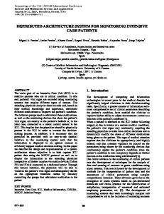
A. The Transit Network The transit system that we have considered is represented as a one-way loop with K stops and N buses, as shown in Figure 1. We will state our assumptions while presenting the specific problem scenarios. N-1

N

3…

2

Stop

…

Bus

1 K

K-1

3

1 2 Figure 1. The Transit Network Used In This Work

B. List of Symbols Here we list the prominent symbols used in this paper.

l

– Loop index

a i , k ,l

– Arrival time of bus i on its lth loop at stop k

d i , k ,l

– Departure time of bus i on its lth loop from stop k

λ k (t ) – Passenger arrival rate at stop k at time t Bi ,k ,l

– Number of passengers departing stop k on bus i on its lth loop

Gi , k ,l

– Number of passengers alighting bus i on its lth loop at stop k

t m ,k

– Arrival time of passenger m at stop k, m ∈ Pk (t1 , t 2 )

bm ,k

– Boarding time of passenger m at stop k, m ∈ Pk (t1 , t 2 )

M k (t1 , t 2 ) – Number of passengers who have arrived at stop k over an interval (t1 , t 2 ) Pk (t1 , t 2 ) – Set of passengers who have arrived at stop k over an interval (t1 , t 2 )

C. Objective Function

3

In our model, we consider two types of waiting costs: off-bus and on-bus costs. The former cost is incurred when a passenger is at a stop waiting for a bus to arrive. The latter cost is incurred when the passenger is on-board a bus but is waiting for the bus to depart from a stop. In this case, the bus may be held due to waiting for other passengers to arrive. We differentiate between these two cost components because passengers waiting outside the bus may experience more inconvenience than those waiting inside, especially in inclement weather conditions. We do not consider the passenger travel costs in this paper because: 1) it is difficult to track an individual passenger through his/her entire trip; 2) from a control point of view, travel control can be treated as an independent problem and can be addressed separately. 1. The off-bus waiting cost, WFi ,k ,l , incurred due to the passengers who will be boarding the ith bus on its lth loop of travel, arriving at the kth stop, is given by

WFi ,k ,l =

∑ f (b

F m,k m∈Pk (d i −1, k , l , ai , k , l )

− t m ,k )

(1)

where f F (t ) is the cost function for an individual off-bus passenger, f F (0) = 0 , f F (t ) ≥ 0 for t ≥ 0 , and t is the waiting time. 2. The on-bus waiting cost, WN i , k ,l , incurred due to the passengers who are already on-board the ith bus on its lth loop of travel, arriving at the kth stop and are waiting for the bus to continue moving to the next stop, is given by WN i , k ,l = (Bi , k −1,l − Gi , k ,l )⋅ f N (d i , k ,l − ai , k ,l ) +

∑ f (d

N i , k ,l m∈Pk (d i −1,k ,l , d i ,k ,l )

− bm , k )

(2)

where f N (t ) is the cost function for an individual on-bus passenger, f N (0) = 0 , f N (t ) ≥ 0 for t ≥ 0 . Note that passengers at their boarding stops may also have an on-bus cost if the bus is not dispatched immediately after their boarding. K t Possible nonlinear structures for the functions f F (t ) and f N (t ) are: f F (t ) = K 1F t K 2 F e 3 F ,

f N (t ) = K 1N t K 2 N e K 3 N t . If we set K 1F = K 1N = K 2 F = K 2 N = 1 and K 3 F = K 3 N = 0 , then we have f F (t ) = t and f N (t ) = t . Here K.. are parameters of the cost model chosen based on the context. Our objective is to minimize the average waiting cost of passengers, including both off-bus and on-bus costs, by appropriately controlling d i ,k ,l ’s. After all buses have traveled through Q loops over time interval [t1 ,t 2 ] , the objective function may be expressed as Q

N

K

min C = ∑∑∑ (WFi , k ,l + WN i , k ,l ) l =1 i =1 k =1

K

∑ M (t , t ) k =1

k

1

2

4

(3)

III. REAL-TIME DISTRIBUTED CONTROL APPROACH

A. Architecture Our MAS architecture mainly consists of two types of agents – Stop Agent and Bus Agent, as schematically shown in Figure 2 (a) . A Stop Agent represents the activity at a given stop, and maintains knowledge of several neighboring stops. This knowledge may be used by a Bus Agent to negotiate with several Stop Agents to get an optimal solution covering a wider range. A Bus Agent interacts with a Stop Agent, when it is at or near a particular stop. At each stop, an APC (Automatic Passenger Counter) is used to count the passengers getting on and off. A WAN (Wide Area Network) is required for communication between stops to exchange information, e.g. the most recent bus departure time, the number of passengers at the stops, etc. Information from these ITS devices will be fed to the on-bus computer as well as a central computer located at a control station in order to conduct the negotiation via wireless communication. AVI (Automatic Vehicle Identification) or GPS (Global Position System) may also be very helpful, especially for those buses traveling between stops. On-Bus Computer

Bus Agent Bus Agent

Stop Agent

Stop Agent

Wireless Communication

Bus Agent

Central Computer

Stop Agent

APC

WAN

(a)

(b) Figure 2. (a) MAS Architecture, (b) Basic Hardware Environment to Implement Our Control Approach.

B. Negotiation Our negotiation algorithm is based on marginal cost calculations, and is similar to the one used by Sandholm (1993) in his TRACONET (TRAnsportation COoperation NET). We note that the negotiation procedure is independent of the number of times the bus has been on the loop. Thus, for notational convenience, we drop the index l in this discussion. Holding a bus at a stop increases the on-bus cost. Simultaneously, it will decrease the future off-bus cost, because the

(

)

interval d i ,k , a i +1,k tends to become shorter as holding decreases the headway between buses i and i+1. A local optimal di,k for minimizing the sum of the on-bus and off-bus costs at a particular stop k for bus i may exist when the

5

on-bus marginal cost, MN i, k (t ) , equals the expected off-bus marginal cost, MFi +1,k (t ) . In other words, a necessary condition for the optimality of dispatching is

( )

( )

*

MN i ,k d i ,k = MFi +1,k d i ,k

*

(4)

Suppose, at time t, negotiation is taking place between bus i and stop k. The on-bus marginal cost, MN i, k (t ) , is given as

MN i ,k (t ) =

∂WN i ,k (t ) ∂t

=

 ∂  f N (t − bm ,k ) (Bi ,k −1 − G i ,k ) ⋅ f N (t − a i ,k ) + ∑ ∂t  m∈Pk (d i −1, k ,t ) 

= (Bi ,k −1 − G i ,k ) ⋅ f N′ (t − a i ,k ) +

(5)

∑ f ′ (t − b )

N m∈Pk (d i −1, k ,t )

m,k

For obtaining the expected off-bus marginal cost, MFi +1, k (t ) , we first determine the conditional expectation of the off-bus cost of passengers arriving at stop k should the bus i leave at time t as ai +1, k ∞ E {WFi +1,k t}= ∫ p ai +1, k (a~i +1,k t ) ∫ λ k (τ ) f F (a~i +1,k − τ )dτ da~i +1,k t t   ~

(

)

where p ai +1, k a~i +1,k t is the conditional probability density function of the arrival times of the next bus (i+1) if bus i leaves stop k at time t. Note that the expression in the innermost integral represents off-bus waiting costs of passengers that arrive within an infinitesimal interval at time τ. Then we obtain the expected off-bus marginal cost as a~i +1, k ∂ ∂ ∞ E (WFi +1,k t ) = − ∫ p ai +1, k (a~i +1,k t ) ∫ λk (τ ) f F (a~i +1,k − τ )dτ da~i +1,k t t   ∂t ∂t ∞ = p ai +1, k (t t )λ k (t ) f F (0) + λ k (t )∫ p ai +1, k (a~i +1,k t ) f F (a~i +1,k − t )da~i +1,k

MFi +1,k (t ) = −

(6)

t

∞ = λ k (t )∫ p ai +1, k (a~i +1,k t ) f F (a~i +1,k − t )da~i +1,k t

(

)

A close form expression for the RHS of (6) is possible for appropriate types of f F (t ) and p ai +1, k a~i +1,k t . For example, if f F (t ) = t , we have

MFi +1,k (t ) = λk (t ) f F (a i +1,k − t )

(7)

(

)

where ai +1,k is the expected arrival time of the next bus. Also, if the p ai +1, k a~i +1,k t is concentrated around a i +1,k ,

(

)

and if f F a~i +1,k − t does not vary significantly in the neighborhood of a i +1,k − t , then (7) becomes a good

~ approximation for (6). Realistically speaking, estimation of a i +1,k is nontrivial, and the use of ITS devices can enhance the accuracy of its estimation. In the absence of any real-time information, a i +1,k becomes the best predictor

~ of a i +1,k . Based on the foregoing marginal cost calculations, we have the following negotiation algorithm.

6

Algorithm 1: Step1. At negotiation time, t , the Bus Agent and the Stop Agent calculate their marginal cost, MN i, k (t ) and

MFi +1,k (t ) , respectively; Step2. If MN i , k (t ) ≥ MFi +1, k (t ) , dispatch the bus immediately; otherwise, hold the bus and increment the negotiation time as t = t + ∆t , where ∆t is a small time interval.

Assuming the last dispatching time as well as the next dispatching time is fixed, Algorithm 1 guarantees only a necessary condition for optimal dispatching. In the following section, we will show that under some reasonable assumptions, the algorithm also guarantees the sufficient condition for optimal dispatching.

C. Local Optimality Conditions The negotiation algorithm based on marginal cost calculations does not guarantee the optimality, for it validates only the necessary conditions. However, if (7) is used to calculate MFi +1, k (t ) and a few other mild assumptions hold, we can then make the conditions also sufficient for the negotiation procedure.

Lemma 1 If f N (t ) is a convex function, then the on-bus marginal cost, MN i, k (t ) , is a monotonically increasing function of t.

Proof: Suppose a i , k ≤ t1 < t 2 ≤ a i +1, k , then

MN i , k (t2 ) − MN i , k (t1 ) = (Bi , k −1 − Gi , k )[ f N′ (t2 − ai , k ) − f N′ (t1 − ai , k )] +

∑ [ f ′ (t

N m∈Pk (a i , k , t1 )

2

− bm, k ) − f N′ (t1 − bm, k )] +

∑ f ′ (t

N m∈Pk (t1 , t 2 )

2

− bm, k )

Since f N (t ) is a convex function, the first and second items on the right side of the above equation are non-negative. Also notice that f N (0 ) = 0 , f N (t ) ≥ 0 for t ≥ 0 , and f N′ (t ) ≥ 0 for t ≥ 0 . So the third item is non-negative as well. Therefore we have MN i , k (t 2 ) − MN i , k (t1 ) ≥ 0 , and have proved Lemma 1.■

Lemma 2 If (i) f F (t ) is a non-decreasing function, and (ii) the passenger arrival rate, λ k (t ) , does not increase over an interval

[t1 ,t 2 ] (a i ,k

≤ t1 < t 2 ≤ a i +1,k ) , (iii) MFi +1,k (t ) is given by (6), then the expected off-bus marginal cost decreases

monotonously over [t1 ,t 2 ] .

7

Proof for Lemma 2 becomes apparent from examining the terms in the RHS of (6). ■ We know that holding a bus reduces the off-bus costs but can increase the on-bus costs. If we perceive the decrement of the off-bus cost as an offer and the increment of the on-bus cost as a price, then our effort is to maximize the net profit. Lemma 1 and Lemma 2 provide us with a direct solution. Lemma 1 says that the price is convex, and Lemma 2 says that the offer is concave (see Figure 3). Hence, the optimality arises when the slopes of the offer and the price are equal.

Theorem 1 If (i) f N (t ) is a convex function, (ii) f F (t ) is a non-decreasing function, (iii) the passenger arrival rate, λ k (t ) , does

(

)

not increase over an interval [t1 ,t 2 ] a i ,k ≤ t1 < t 2 ≤ a i +1,k , and (iv) MFi +1,k (t ) is given by (7), then the optimal

( )

( )

dispatching time, d i*,k , in [t1 , t 2 ] , occurs when the marginal costs are equal, i.e. MN i , k d i*,k = MFi +1, k d i*,k .■

Offer

Price

ai,k

di,k* ai+1,k Figure 3. Optimality Condition

Most of the conditions for Theorem 1 are reasonable. However, we assume the passenger arrival rate to be nonincreasing over the negotiation period. This condition will hold for a stationary process, and not necessarily for a non-stationary process. However, in real world situations, the passenger arrival rate most often has only one peak between successive bus arrivals, occurring just before a scheduled bus arrival time. The optimal dispatching time is most likely to be after that peak and before the next peak. Thus, the negotiation algorithm based on marginal cost calculations is still relevant.

D. Hyperopic Considerations Although Algorithm 1 is efficient for negotiation between a Stop Agent and a Bus Agent, we still have no guarantee of global optimality. This is because optimality of each single stop does not imply optimality of the entire line. For example, when a bus is being held at a stop, hoping that its profit will increase, many passengers, who wait for it at 8

downstream stops, will bear additional costs. The system has to be penalized for the “myopia” of this bus. In other words, holding a bus i at stop k has a double impact on the downstream stops – it will increase the cost of passengers who are waiting for the bus while maybe decreasing the cost of passengers who are waiting for the next bus. A wider range of negotiation may be needed to overcome this “myopia”. A Bus Agent may not only negotiate with the stop at which it is held, but it may also need to negotiate with several downstream stops, where passengers are waiting. A further improvement can be made if we set a Line Agent to supervise the conditions of the entire line. Suppose when bus i is held at stop k, passengers at stop k+1, …, k+m, are also waiting for it to arrive. Then the approximation of the expected off-bus cost at stop k+j ( 1 ≤ j ≤ m ) is given as

WFi ,k + j (t ) =

f (a ∑ ( ) F

m∈Pk + j d i −1, k + j , t

WFi +1,k + j (t ) = ∫

a i + 1, k + j

ai , k + j

i ,k + j

− d i −1,k + j ) + ∫

ai , k + j

t

λk + j (τ ) f F (a i ,k + j − τ )dτ

λ k + j (τ ) f F (a i +1,k + j − τ )dτ

(8)

(9)

Here, we treat the bus travel time to be deterministic. We then have

MFi ,k + j (t ) = −

f ′ (a ∑ ( ) F

m∈Pk + j d i −1, k + j ,t

i ,k + j

− d i −1,k + j ) − ∫

ai , k + j

t

λk + j (τ ) f F′ (a i ,k + j − τ )dτ

MFi +1,k + j (t ) = λ k + j (a i ,k + j ) f F (a i +1,k + j − a i ,k + j )

(10) (11)

The optimum dispatching time, d i*,k , satisfies

MN i , k (d i*,k ) = MFi +1,k (d i*,k ) + ∑ (MFi ,k + j (d i*,k ) + MFi +1,k + j (d i*,k )) m

(12)

j =1

The underlying assumption here is that neither bus i nor bus i+1 will be held at downstream stops. Equation (12) treats the costs at the current stop and downstream stops equally. However, we may want to deal with them with different weights,

MN i , k (d i*,k ) = MFi +1,k (d i*,k ) + ∑ µ j (MFi ,k + j (d i*,k ) + MFi +1,k + j (d i*,k )) m

(13)

j =1

where µ j is weight for stop k+j. Since the estimations for downstream stops are less reliable, we may set smaller weights for them. If we set µ j = 0 for all j, then we ignore the downstream stops and have the same equation as in

Theorem 1. Based on (13), we have the following modified negotiation algorithm:

Algorithm 2: Step1. At negotiation time, t , the Bus Agent i, which is on stop k, calculates its marginal cost MN i, k (t ) using (4);

9

Step2. At the same time, the Stop Agent k calculates its marginal cost MFi +1, k (t ) using (6), it also communicates with the downstream stops, where bus i-1 has already departed from, informing them the estimated arrival time of bus i and having them to calculate their marginal costs, MFi , k + j (t ) , MFi +1, k + j (t ) (j=1,2,…, m, where m is the number of involved downstream stops), based on their local data and using (10) and (11);

Step3. If MN i , k (t ) ≥ MFi +1, k (t ) + ∑ µ j (MFi , k + j (t ) + MFi +1, k + j (t )) , dispatch bus i immediately; otherwise, hold the m

j =1

bus and renew the negotiation time t = t + ∆t , where ∆t is a small time interval.

Note that further improvements can be made by considering the downstream stops where bus i-1 has not yet arrived. This is a subject for future research.

IV. SIMULATION STUDIES

A. Simulation System To verify the efficiency of our real-time distributed framework, we developed a simulation system to test and compare the performance of our framework with that of other simple strategies, namely, On-Schedule and EvenHeadway. The simulations were implemented in the AweSim environment. We set up a loop with NS stops and NB buses as shown in Figure 1. Passenger arrivals at each stop are assumed to be Poisson processes (can be either stationary or non-stationary). Also, the passenger alighting ratio at each stop k is given by ρ k . The travel times between two adjacent stops are identically distributed lognormal random variables with a mean of TBS and variance of σ 2 . This is a reasonable assumption as many of the urban transit loops have large segments with near-equal travel times. Cost functions are f F (t ) = f N (t ) = t . We also consider the dwelling (boarding only) time for each passenger, DW, which is a constant. In all scenarios, we make 10 simulation runs with each being run for 1200 minutes. We test and compare the following four strategies: 1. No-Wait strategy: Buses are not held at stops, and they leave immediately after passenger unloading and loading. 2. Headway-based (Even-Headway) strategy: A bus is held at a stop (beyond unloading and loading) in order to make the headway between the current and the preceding bus equal to that between the current and the succeeding bus.

10

3. Schedule-based (On-Schedule) strategy: A bus is held at a stop (beyond unloading and loading) only if it arrives earlier than the scheduled arrival time. Note that in most transit systems the scheduled arrival time is typically longer than the expected actual arrival time since there is usually some slack in the schedule (Dessouky, et al., 1999). That is, transit agencies incorporate slack between major stops/checkpoints to ensure schedule adherence. If TBS is the expected travel time between two stops, then the scheduled travel time is TBS ⋅ (1 + s ) , where s is the slackness. 4. Negotiation strategy using marginal costs: Buses are held (beyond unloading and loading) according to

Algorithm 2.

B. Simulation for Stationary Passenger Arrivals We use the following physical parameters of the transit system: NS = 10 , NB depends on the scenario, TBS = 5 min ,

σ 2 = 4 , ρ k = 0.4 , DW = 0.05 min , passenger arrival rate λ = 1.0 / min and is identical for all stops. For the Negotiation strategy, we set µ k = 1 for all k. 10. 00% 8. 00%

Savings

6. 00% 4. 00% 2. 00% 0. 00% 5

10

15

20

25

30

- 2. 00% Scheduled Headway On Schedule Even Headway

Negotiation

Figure 4. Savings of Different Strategies Relative to No-Wait Strategy

In Scenario 1, we assume there is sufficient slack only at the terminal stop in the schedule so that all buses leave on time at the terminal stop. This scenario is equivalent to viewing the route as a straight line instead of as a loop. We assume a slackness, s, for all experiments in this scenario to be 0.3. This is comparable to the amount of slack found on bus lines in Los Angeles County (Dessouky et al., 1999). We have simulated the route with different headways. Figure 4 shows the savings, relative to the No-Wait strategy, under different headways. As the figure shows, the Negotiation strategy outperforms the other strategies especially when the headway is less than 10 minutes. As

11

expected, the gap between the Negotiation and On-Schedule strategies becomes smaller as the headway increases. Note that under random travel times and small scheduled headways, holding buses to meet schedules or to even out headways will lead to inferior performance compared to the No-Wait strategy (as reflected in negative savings in Figure 4) as only the early buses are held and the late buses are not allowed to pre-empt their subsequent arrivals. 20 Area2

18

Average Wait

16 Area3

14

Area1

12 10 Area4

8 6 8

9

10

11

No Wait

12

13 14 15 16 Scheduled Headway On Schedule Even Headway

17

18

19

20

Negotiation

Figure 5. Determine Appropriate Slackness

In contrast with scenario 1, we assume in Scenario 2 that buses may leave late at the terminal stop. Once a bus is late, it also affects the performance in the subsequent loops. The relationship between slackness, scheduled headway and system parameters for the loop is SH = TBS ⋅ (1 + s ) ⋅ NS NB , where SH is the scheduled headway.

We first try to determine the best level of s for the different strategies. Figure 5 shows that area 3 is the best working area for all strategies, i.e. slackness, s, should be between 0.2 and 0.3 considering that TBS=10. This result is consistent with the observation of Dessouky et al. (1999) on Los Angeles County routes, which have slackness of 0.25. In area 1 (a system suffering sudden bus breakdowns may lie in this area), the No-Wait and On-Schedule strategies are unstable since the buses cannot make the schedule under these slackness levels. However, the Even-Headway and Negotiation strategies are stable in this region. That is, under these strategies, the average waiting times reach near steady state values. This is because Even-Headway and Negotiation strategies are schedule-independent strategies and have relatively strong self-adjustment ability. In this case, the actual headway is larger than the scheduled headway but the coefficient of variation of actual headway, C (H )2 , are almost constant and small. In area 2, the 12

average waiting times for the No-Wait and On-Schedule strategies decrease significantly as the slackness increases. In area 3, all strategies are stable and this area contains the best level of slackness in the schedule. Area 4 shows that as the slackness continues to increase the average waiting time will then increase. In summary, a scheduled headway of 12 minutes minimizes the average waiting time for this scenario, and at this slackness, all the strategies except NoWait perform equally well.

C. Simulation for Non-Stationary Passenger Arrivals

In reality, passenger arrivals are often non-stationary. We consider two kinds of non-stationary arrivals: 1) Random events causing random bursts of passenger arrivals: Some examples include audiences emerging in random bursts after short events or shows in amusement parks such as Disneyland, movie complexes, and downtown corridors, as well as passenger arrivals at transfer stops of a transit network. In these cases, a large number of passengers arrive when the random event happens (i.e., the show ends or the bus carrying transfer passengers arrives). 2) Passengers being aware of schedules: Here the arrivals are non-stationary and follow a specific pattern (as shown in Figure 10). Such a phenomenon is common whenever SH > 13 min (Bowman and Turnquist, 1981). Scenario – Passenger Arrivals in Bursts Here, the passenger arrival rate consists of random peaks representing bursts of passenger arrivals. We assume that each peak is a gaussian function of time, and the length of each peak period is exponentially distributed with mean of α . However, the average arrival rate λ for each period is a constant. Hence, the arrival rate during each period may be expressed as

 (t − t p )2   λ L ⋅ exp −  2σ 2  p   , t − L ≤ t < t + L  λ (t ) = t + L  p  p p 2 2 2   (τ − t p )2  ∫ L exp − 2σ 2 dτ p tp − 2  

(14)

where L is the length of the period, t p is the midpoint of the period (i.e., peak time), and σ p is the variance of the 2

normal distribution. A typical passenger arrival rate pattern is shown in Figure 6.

13

18 16 14 Arrival Rate

12 10 8 6 4 2 0 500

520

540

560

580

600

Time

Figure 6. Passenger Arrival Rate with Random Bursts

The parameters are kept the same as the earlier case, and we assume there is sufficient slack at the terminal stop so that the buses can always depart on-time at the terminal stop. For the Negotiation strategy, we have set µ k = 0 for all k, because the passenger arrivals at downstream stops are non-stationary with random bursts; as a result, the estimates of future passenger arrivals become unreliable. Hence, prediction of marginal costs at downstream stops does not help much, and may even worsen the solution quality, in this situation. First, we have tested the efficiency of the strategies under different average arrival rates of passengers. We assume

σ p 2 = 1.0 for all situations. The simulation results are shown in Figure 7, again as a percentage savings over the No-wait strategy. The result shows that the Negotiation strategy can save much more than the other strategies when the average arrival rate is less than 1.2/min. However, the performance of all strategies (except No-Wait strategy) are close to each other for average arrival rates greater than 1.2. Overall, the savings of the Negotiation strategy are greater in this nonstationary case than for the previous stationary scenario. Next, we assume that the passenger average arrival rates are identical for all stops at λ = 1.0 / min . We test the performance of different strategies under different σ p values, ranging from 1.0 min 2 to 64 min 2 . We compare 2

the savings of different strategies relative to the No-Wait Strategy. The simulation results are summarized in Figure 8. It is evident that the larger the σ

2 p

, the closer the passenger arrivals will be to a stationary process, and the less

the benefit of the Negotiation strategy can obtain.

14

Next, we have simulated transit lines with different headways ranging from 5 min up to 30 min. Here, we assume that

λ = 1.0 / min and σ p 2 = 1.0 for all situations. Our simulation results summarized in Figure 9 reveal that the Negotiation strategy outperforms other strategies for all tested headways, especially for SH < 15 min.

16. 00%

Savings

12. 00%

8. 00%

4. 00%

0. 00% 0

0. 2

0. 4

0. 6

0. 8

1

1. 2

1. 4

1. 6

1. 8

2

- 4. 00% Average Arrival Rate On Schedule Even Headway

Negotiation

Figure 7. Savings of Different Strategies under Different λ

16. 00%

Savings

12. 00%

8. 00%

4. 00%

0. 00% 1

2

4

8 10

16

32

64

Variance of Normal Distribution On Schedule Even Headway Negotiation

Figure 8. Savings of Different Strategies under Different

15

σ p2

100

24. 00% 20. 00%

Savings

16. 00% 12. 00% 8. 00% 4. 00% 0. 00% 5

10

15

20

25

30

- 4. 00% Scheduled Headway On Schedule Even Headway

Negotiation

Figure 9. Savings of Different Strategies under Different Headways

Scenario – Passenger Arrivals with Awareness of Schedule As we earlier mentioned, many researchers argue that passengers become aware of the schedules when the headway exceeds 13 minutes. A representative probability density function of passenger arrival time assuming a bus scheduled arrival time of 10 clock-time units, is shown in Figure 10 is obtained using the utility theoretic construct of Bowman and Turnquist (1981).

Probability Density

0.16 0.14 0.12 0.1 0.08 0.06 0

2

4

6

Arrival Time

8

10

Figure 10. The Density Function of Passenger Arrival Times based on Utility Theory

We have simulated a straight line configuration for this scenario with the same physical parameters as the previous scenarios. We test the performance with headways ranging from 10 minutes to 30 minutes. The simulation results

16

(Figure 11) show that the Negotiation strategy performs as well as the On-Schedule strategy, while the EvenHeadway strategy performs much worse (even worse than the No-Wait strategy for large headways). Note that when passengers time their arrival to match the scheduled bus departure time, it is unlikely that any other strategy can consistently outperform the On-schedule strategy.

20. 00% 15. 00%

Savings

10. 00% 5. 00% 0. 00% 10

15

20

25

30

- 5. 00% - 10. 00% On Schedule

Scheduled Headway Even Headway

Negotiation

Figure 11. Performance Comparison of Different Strategies with Aware Passengers

V. CONCLUDING REMARKS

The bus-holding problem has been studied for many years. Various strategies have been presented to address this problem. The most common and the simplest method is the On-Schedule strategy. It utilizes only the stationary statistics but not real-time information. This strategy works best when passengers time their arrivals to the scheduled departure time of the bus. The Even-Headway strategy uses only the real-time information regarding the departure time of the last bus. This strategy works best under stationary passenger arrivals with short headways. In the recent years, many studies focus on developing real-time control strategies, intending to obtain better coordination of the system. However, none of the available methods is adequately robust for application in a wide range of transit scenarios.

17

We have developed a negotiation-based framework, wherein stops and buses act as agents. They negotiate based on their marginal costs. Our work proves that under some reasonable assumptions, the framework can find local optimal dispatching times. Our distributed holding control approach distinguishes itself for its ability to harness real-time information and to make decisions directly based on the marginal waiting cost. To verify the efficiency of our strategy, we also developed a simulation system. We conducted simulations for stationary as well as different kinds of non-stationary passenger arrivals. The simulation results verify that our framework is robust and adequate for coordination in a wide range of transit environments.

Another advantage of our Negotiation strategy is that it can consider the waiting cost of continuing passengers with different types of cost functions. In other words, the negotiation algorithm is more flexible and generic compared to the existing transit control methods. Our simulations also show that simple strategies, i.e. On-Schedule and EvenHeadway strategies, are adequate for a narrow range of transit situations. However, for non-stationary situations such as those present in amusement parks, airports, schools, etc., these simple strategies are not adequate and our negotiation-based framework provides significantly better solutions. Although the current objective is to minimize waiting times, we can, with a little additional efforts, can expand our approach to minimize excessive lateness and overcrowding, which are considered among the major issues with modern transportation systems.

ACKNOWLEDGMENT

We acknowledge METRANS, for its kind support of this research.

REFERENCES

[1]

Barnett, A. (1974). “On Controlling Randomness in Transit Operations,” Transportation Science, Vol. 8, pp. 102-116.

[2]

Barnett, A. (1978). “Control Strategies for Transport Systems with Nonlinear Waiting Costs,” Transportation Science, Vol. 12, pp. 119-136.

[3]

Bazan, A. (1995). “A Game-Theoretic Approach to Distributed Control of Traffic Signals,” Proc. First International Conf. on Multi-Agent Systems, San Francisco, CA, USA, pp. 439.

[4]

Bowman, L. A., and M. A. Turnquist (1981). “Service frequency, Schedule Reliability and Passenger Wait Times at Transit Stops,” Transportation Research, Vol. 15A, pp. 465-471.

[5]

Dessouky, M., R. Hall, A. Nowroozi, and K. Mourikas (1999). “Bus Dispatching at Timed Transfer Transit Stations Using Bus Tracking Technology,” Transportation Research, Vol. 7C, pp. 187-208.

[6]

Eberlein, X. J., N. H. M. Wilson, C. Barnhart, and D. Bernstein (1998). “The Real-Time Deadheading Problem in Transit Operations Control,” Transportation Research, Vol. 32B, pp. 77-100.

18

[7]

Eberlein, X. J., N. H. M. Wilson, D. Bernstein (2001). “The Holding Problem with Real-Time Information Available,” Transportation Science, Vol. 35, No. 1, pp. 1-18.

[8]

Jolliffe, J. K., and T. P. Hutchinson (1975). “A Behavioral Explanation of Association Between Bus and Passenger Arrivals at a Bus Stop,” Transportation Science, Vol. 9, pp. 248-292.

[9]

Kohout, R. and K. Erol (1999). “In-Time Agent-Based Vehicle Routing with a Stochastic Improvement Heuristic,” Proc. Sixteenth National Conf. on Artificial Intelligence (AAI-99). Eleventh Innovative Applications of Artificial Intelligence Conf. (IAAI-99), Orlando, FL, USA, pp. 864-869.

[10]

Newell, G. F. (1971). “Dispatching Policies for a Transportation Route”, Transportation Science, Vol. 5, pp. 91-105.

[11]

Newell, G. F. (1974). “Control of Pairing of Buses on a Public Transportation Route, Two Buses, One Control Point,” Transportation Science, Vol. 8, pp. 248-264.

[12]

Okrent, M. M. (1974). “Effects of Transit Service Characteristics on Passenger Waiting Time,” M.S. Thesis, Northwestern University, Department of Civil Engineering, Evanston, Illinois.

[13]

Osuna, E. E., and G. F. Newell (1972). “Control Strategies for an Idealized Public Transportation System,” Transportation Science, Vol. 6, pp. 52-72.

[14]

Powell, W. B. (1983). “Bulk Service Queues with Deviations from Departure Schedules: The Problem of Correlated Headways,” Transportation Research, Vol. 17B, pp. 221-232.

[15]

Powell, W. B. (1985). “Analysis of Bus Holding and Cancellation Strategies in Bulk Arrival, Bulk Service Queues,” Transportation Science, Vol. 6, pp. 52-77.

[16]

Sandholm, T. (1993). “An Implementation of the Contract Net Protocol Based On Marginal Cost Calculations,” Proc. of the Eleventh National Conference on Artificial Intelligence, Washington, DC, USA, pp. 256-262.

[17]

Satapathy, G., and S. R. T. Kumara (2000). “Negotiation for Transportation Tasks with Stochastic Payoffs,” Computer in Industry, 42(2-3), pp. 193-202.

[18]

Schiemek, P. (2000), “BRT Reference Guide,” DOT Archives, http://brt.uolpe.dot.gov/guide/

19

Biographical Sketches

Jiamin Zhao, is a Doctoral Candidate in the Department of Industrial and Systems Engineering. His research interests are in developing effective optimization and control strategies for transit operations. He got his B.S. in Department of Automation at Tsinghua University, China. Satish Bukkapatnam, Ph.D., is an Assistant Professor of Industrial and Systems Engineering at the University of Southern California. His research has yielded methods to build models for monitoring and control of complex nonlinear dynamic systems using data from sensor signals, specifically for applications in manufacturing and, recently, transportation. He has over 35 refereed publications on these topics, and his research has received support from National Science Foundation and the Office of Naval Research. He received his MS and Ph.D. degrees in Industrial and Manufacturing Engineering from Pennsylvania State University. PI: Maged M. Dessouky, Ph.D., is an Associate Professor of Industrial and Systems Engineering, University of Southern California. Prior to joining USC, Dr. Dessouky was employed at Hewlett-Packard (Systems Analyst), Bellcore (Member of Technical Staff), and Pritsker Corporation (Senior Systems Analyst). Dr. Dessouky research interests are in the theoretical and practical understanding of models and heuristic methods for transportation system optimization. He is currently an investigator on several NSF transit-related projects. He received his Ph.D. in Industrial Engineering from University of California, Berkeley, and M.S. and B.S. degrees from Purdue University. He is the Area Editor of Planning and Scheduling for the International Journal of Computers & Industrial Engineering.

20