Distributed Batch Gaussian Process Optimization

Distributed Batch Gaussian Process Optimization Erik A. Daxberger 1 Bryan Kian Hsiang Low 2

Abstract This paper presents a novel distributed batch Gaussian process upper confidence bound (DB-GP-UCB) algorithm for performing batch Bayesian optimization (BO) of highly complex, costly-to-evaluate black-box objective functions. In contrast to existing batch BO algorithms, DBGP-UCB can jointly optimize a batch of inputs (as opposed to selecting the inputs of a batch one at a time) while still preserving scalability in the batch size. To realize this, we generalize GP-UCB to a new batch variant amenable to a Markov approximation, which can then be naturally formulated as a multi-agent distributed constraint optimization problem in order to fully exploit the efficiency of its state-of-the-art solvers for achieving linear time in the batch size. Our DB-GP-UCB algorithm offers practitioners the flexibility to trade off between the approximation quality and time efficiency by varying the Markov order. We provide a theoretical guarantee for the convergence rate of DB-GP-UCB via bounds on its cumulative regret. Empirical evaluation on synthetic benchmark objective functions and a real-world optimization problem shows that DB-GP-UCB outperforms the stateof-the-art batch BO algorithms.

1. Introduction Bayesian optimization (BO) has recently gained considerable traction due to its capability of finding the global maximum of a highly complex (e.g., non-convex, no closedform expression nor derivative), noisy black-box objective 1

Ludwig-Maximilians-Universität, Munich, Germany. A substantial part of this research was performed during his student exchange program at the National University of Singapore under the supervision of Bryan Kian Hsiang Low and culminated in his Bachelor’s thesis. 2 Department of Computer Science, National University of Singapore, Republic of Singapore. Correspondence to: Bryan Kian Hsiang Low . Proceedings of the 34 th International Conference on Machine Learning, Sydney, Australia, PMLR 70, 2017. Copyright 2017 by the author(s).

function with a limited budget of (often costly) function evaluations, consequently witnessing its use in an increasing diversity of application domains such as robotics, environmental sensing/monitoring, automatic machine learning, among others (Brochu et al., 2010; Shahriari et al., 2016). A number of acquisition functions (e.g., probability of improvement or expected improvement (EI) over the currently found maximum (Brochu et al., 2010), entropybased (Villemonteix et al., 2009; Hennig & Schuler, 2012; Hernández-Lobato et al., 2014), and upper confidence bound (UCB) (Srinivas et al., 2010)) have been devised to perform BO: They repeatedly select an input for evaluating/querying the black-box function (i.e., until the budget is depleted) that intuitively trades off between sampling where the maximum is likely to be given the current, possibly imprecise belief of the function modeled by a Gaussian process (GP) (i.e., exploitation) vs. improving the GP belief of the function over the entire input domain (i.e., exploration) to guarantee finding the global maximum. The rapidly growing affordability and availability of hardware resources (e.g., computer clusters, sensor networks, robot teams/swarms) have motivated the recent development of BO algorithms that can repeatedly select a batch of inputs for querying the black-box function in parallel instead. Such batch/parallel BO algorithms can be classified into two types: On one extreme, batch BO algorithms like multi-points EI (q-EI) (Chevalier & Ginsbourger, 2013), parallel predictive entropy search (PPES) (Shah & Ghahramani, 2015), and the parallel knowledge gradient method (q-KG) (Wu & Frazier, 2016) jointly optimize the batch of inputs and hence scale poorly in the batch size. On the other extreme, greedy batch BO algorithms (Azimi et al., 2010; Contal et al., 2013; Desautels et al., 2014; González et al., 2016) boost the scalability by selecting the inputs of the batch one at a time. We argue that such a highly suboptimal approach to gain scalability is an overkill: In practice, each function evaluation is often much more computationally and/or economically costly (e.g., hyperparameter tuning for deep learning, drug testing on human subjects), which justifies dedicating more time to obtain better BO performance. In this paper, we show that it is in fact possible to jointly optimize the batch of inputs and still preserve scalability in the batch size by giving practitioners the flexibility to trade off BO performance for time efficiency.

Distributed Batch Gaussian Process Optimization

To achieve this, we first observe that, interestingly, batch BO can be perceived as a cooperative multi-agent decision making problem whereby each agent optimizes a separate input of the batch while coordinating with the other agents doing likewise. To the best of our knowledge, this has not been considered in the BO literature. In particular, if batch BO can be framed as some known class of multi-agent decision making problems, then it can be solved efficiently and scalably by the latter’s state-of-the-art solvers. The key technical challenge would therefore be to investigate how batch BO can be cast as one of such to exploit its advantage of scalability in the number of agents (hence, batch size) while at the same time theoretically guaranteeing the resulting BO performance. To tackle the above challenge, this paper presents a novel distributed batch BO algorithm (Section 3) that, in contrast to greedy batch BO algorithms (Azimi et al., 2010; Contal et al., 2013; Desautels et al., 2014; González et al., 2016), can jointly optimize a batch of inputs and, unlike the batch BO algorithms (Chevalier & Ginsbourger, 2013; Shah & Ghahramani, 2015; Wu & Frazier, 2016), still preserve scalability in the batch size. To realize this, we generalize GP-UCB (Srinivas et al., 2010) to a new batch variant amenable to a Markov approximation, which can then be naturally formulated as a multi-agent distributed constraint optimization problem (DCOP) in order to fully exploit the efficiency of its state-of-the-art solvers for achieving linear time in the batch size. Our proposed distributed batch GPUCB (DB-GP-UCB) algorithm offers practitioners the flexibility to trade off between the approximation quality and time efficiency by varying the Markov order. We provide a theoretical guarantee for the convergence rate of our DBGP-UCB algorithm via bounds on its cumulative regret. We empirically evaluate the cumulative regret incurred by our DB-GP-UCB algorithm and its scalability in the batch size on synthetic benchmark objective functions and a realworld optimization problem (Section 4).

2. Problem Statement, Background, and Notations Consider the problem of sequentially optimizing an unknown objective function f : D ! R where D ⇢ Rd denotes a domain of d-dimensional input feature vectors. We consider the domain to be discrete as it is known how to generalize results to a continuous, compact domain via suitable discretizations (Srinivas et al., 2010). In each iteration t = 1, . . . , T , a batch Dt ⇢ D of inputs is selected for evaluating/querying f to yield a corresponding column vector yDt , (yx )> x2Dt of noisy observed outputs yx , f (x) + ✏ with i.i.d. Gaussian noise ✏ ⇠ N (0, n2 ) and noise variance n2 .

Regret. Supposing our goal is to get close to the global maximum f (x⇤ ) as rapidly as possible where x⇤ , arg maxx2D f (x), this can be achieved by minimizing a standard batch BO objective such as the batch or full cumulative regret (Contal et al., 2013; Desautels et al., 2014): The notion of regret intuitively refers to a loss in reward from not knowing x⇤ beforehand. Formally, the instantaneous regret incurred by selecting a single input x to evaluate its corresponding f is defined as rx , f (x⇤ ) f (x). Assuming a fixed cost of evaluating f for every possible batch Dt of the same size, the batch and full cumulative regrets are, respectively, defined as sums (over iteration t = 1, . . . , T ) of the smallest instantaneous regret incurred PT by any input within every batch Dt , i.e., RT , t=1 minx2Dt rx , and of the instantaneous regrets incurred by all inputs of every batch Dt , i.e., RT0 , PT P t=1 x2Dt rx . The convergence rate of a batch BO algorithm can then be assessed based on some upper bound on the average regret RT /T or RT0 /T (Section 3) since the currently found maximum after T iterations is no further away from f (x⇤ ) than RT /T or RT0 /T . It is desirable for a batch BO algorithm to asymptotically achieve no regret, i.e., limT !1 RT /T = 0 or limT !1 RT0 /T = 0, implying that it will eventually converge to the global maximum. Gaussian Processes (GPs). To guarantee no regret (Section 3), the unknown objective function f is modeled as a sample of a GP. Let {f (x)}x2D denote a GP, that is, every finite subset of {f (x)}x2D follows a multivariate Gaussian distribution (Rasmussen & Williams, 2006). Then, the GP is fully specified by its prior mean mx , E[f (x)] and covariance kxx0 , cov[f (x), f (x0 )] for all x, x0 2 D, which, for notational simplicity (and w.l.o.g.), are assumed to be zero, i.e., mx = 0, and bounded, i.e., kxx0  1, respectively. Given a column vector yD1:t-1 , (yx )> x2D1:t-1 of noisy observed outputs for some set D1:t 1 , D1 [ . . . [ Dt 1 of inputs after t 1 iterations, a GP model can perform probabilistic regression by providing a predictive distribution p(fDt |yD1:t-1 ) = N (µDt , ⌃Dt Dt ) of the latent outputs fDt , (f (x))> x2Dt for any set Dt ✓ D of inputs selected in iteration t with the following posterior mean vector and covariance matrix: µDt ,KDt D1:t-1(KD1:t-1 D1:t-1+ n2 I) 1 yD1:t-1 , ⌃Dt Dt ,KDt Dt KDt D1:t-1(KD1:t-1 D1:t-1+ n2 I) where KBB0 , (kxx0 )x2B,x0 2B0

1

KD1:t-1 Dt (1) for all B, B 0 ⇢ D.

GP-UCB and its Greedy Batch Variants. Inspired by the UCB algorithm for the multi-armed bandit problem, the GP-UCB algorithm (Srinivas et al., 2010) selects, in each iteration, an input x 2 D for evaluating/querying f that trades off between sampling close to an expected maximum (i.e., with large posterior mean µ{x} ) given the current GP belief of f (i.e., exploitation) vs. that of high predictive un-


certainty (i.e., with large posterior variance ⌃{x}{x} ) to improve the GP belief of f over D (i.e., exploration), that is, maxx2D µ{x} + t1/2 ⌃1/2 {x}{x} where the parameter t > 0 is set to trade off between exploitation vs. exploration for bounding its cumulative regret.

the agents have been assigned to optimize. Complete and approximation algorithms exist for solving a DCOP; see (Chapman et al., 2011; Leite et al., 2014) for reviews of such algorithms.

Existing generalizations of GP-UCB such as GP batch UCB (GP-BUCB) (Desautels et al., 2014) and GP-UCB with pure exploration (GP-UCB-PE) (Contal et al., 2013) are greedy batch BO algorithms that select the inputs of the batch one at a time (Section 1). Specifically, to avoid selecting the same input multiple times within a batch (hence reducing to GP-UCB), they update the posterior variance (but not the posterior mean) after adding each input to the batch, which can be performed prior to evaluating its corresponding f since the posterior variance is independent of the observed outputs (1). They differ in that GPBUCB greedily adds each input to the batch using GP-UCB (without updating the posterior mean) while GP-UCB-PE selects the first input using GP-UCB and each remaining input of the batch by maximizing only the posterior variance (i.e., pure exploration). Similarly, a recently proposed UCB-DPP-SAMPLE algorithm (Kathuria et al., 2016) selects the first input using GP-UCB and the remaining inputs by sampling from a determinantal point process (DPP). Like GP-BUCB, GP-UCB-PE, and UCB-DPP-SAMPLE, we can theoretically guarantee the convergence rate of our DB-GP-UCB algorithm, which, from a theoretical point of view, signifies an advantage of GP-UCB-based batch BO algorithms over those (e.g., q-EI and PPES) inspired by other acquisition functions such as EI and PES. Unlike these greedy batch BO algorithms (Contal et al., 2013; Desautels et al., 2014), our DB-GP-UCB algorithm can jointly optimize the batch of inputs while still preserving scalability in batch size by casting as a DCOP to be described next.

3. Distributed Batch GP-UCB (DB-GP-UCB)

Distributed Constraint Optimization Problem (DCOP). A DCOP can be defined as a tuple (X , V, A, h, W) that comprises a set X of input random vectors, a set V of |X | corresponding finite domains (i.e., a separate domain for each random vector), a set A of agents, a function h : X ! A assigning each input random vector to an agent responsible for optimizing it, and a set W , {wn }n=1,...,N of non-negative payoff functions such that each function wn defines a constraint over only a subset Xn ✓ X of input random vectors and represents the joint payoff that the corresponding agents An , {h(x)|x 2 Xn } ✓ A achieve. Solving a DCOP involves finding the input values of X that maximize the sum of all functions w1 , P . . . , wn (i.e., social N welfare maximization), that is, maxX n=1 wn (Xn ). To achieve a truly decentralized solution, each agent can only optimize its local input random vector(s) based on the assignment function h but communicate with its neighboring agents: Two agents are considered neighbors if there is a function/constraint involving input random vectors that

A straightforward generalization of GP-UCB (Srinivas et al., 2010) to jointly optimize a batch of inputs is to simply consider summing the GP-UCB acquisition function over all inputs of the batch. This, however, results in selecting the same input |Dt | times within a batch, hence reducing to GP-UCB, as explained earlier in Section 2. To resolve this issue but not suffer from the suboptimal behavior of greedy batch BO algorithms such as GP-BUCB (Desautels et al., 2014) and GP-UCB-PE (Contal et al., 2013), we propose a batch variant of GP-UCB that jointly optimizes a batch of inputs in each iteration t = 1, . . . , T according to maxDt ⇢D 1> µDt + ↵t1/2 I[fD ; yDt |yD1:t-1 ]1/2

(2)

where the parameter ↵t > 0, which performs a similar role to that of t in GP-UCB, is set to trade off between exploitation vs. exploration for bounding its cumulative regret (Theorem 1) and the conditional mutual information1 I[fD ; yDt |yD1:t-1 ] can be interpreted as the information gain on f over D (i.e., equivalent to fD , (f (x))> x2D ) by selecting the batch Dt of inputs for evaluating/querying f given the noisy observed outputs yD1:t-1 from the previous t 1 iterations. So, in each iteration t, our proposed batch GP-UCB algorithm (2) selects a batch Dt ⇢ D of inputs for evaluating/querying f that trades off between sampling close to expected maxima P (i.e., with a large sum of posterior means 1> µDt = x2Dt µ{x} ) given the current GP belief of f (i.e., exploitation) vs. that yielding a large information gain I[fD ; yDt |yD1:t-1 ] on f over D to improve its GP belief (i.e., exploration). It can be derived that I[fD ; yDt |yD1:t-1 ] = 0.5 log |I + n 2 ⌃Dt Dt | (Appendix A), which implies that the exploration term in (2) can be maximized by spreading the batch Dt of inputs far apart to achieve large posterior variance individually and small magnitude of posterior covariance between them to encourage diversity. Unfortunately, our proposed batch variant of GP-UCB (2) involves evaluating prohibitively many batches of inputs (i.e., exponential in the batch size), hence scaling poorly in the batch size. However, we will show in this section that our batch variant of GP-UCB is, interestingly, amenable to a Markov approximation, which can then be naturally formulated as a multi-agent DCOP in order to fully exploit the 1 In contrast to the BO algorithm of Contal et al. (2014) that also uses mutual information, our work here considers batch BO by exploiting the correlation information between inputs of a batch in our acquisition function in (2) to encourage diversity.


efficiency of its state-of-the-art solvers for achieving linear time in the batch size. Markov Approximation. The key idea is to design the structure of a matrix Dt Dt whose log-determinant can closely approximate that of Dt Dt , I + n 2 ⌃Dt Dt residing in the I[fD ; yDt |yD1:t-1 ] term in (2) and at the same time be decomposed into a sum of log-determinant terms, each of which is defined by submatrices of Dt Dt that all depend on only a subset of the batch. Such a decomposition enables our resulting approximation of (2) to be formulated as a DCOP (Section 2). At first glance, our proposed idea may be naively implemented by constructing a sparse block-diagonal matrix Dt Dt using, say, the N > 1 diagonal blocks of Dt Dt . Then, log | Dt Dt | can be decomposed into a sum of logdeterminants of its diagonal blocks2 , each of which depends on only a disjoint subset of the batch. This, however, entails an issue similar to that discussed at the beginning of this section of selecting the same |Dt |/N inputs N times within a batch due to the assumption of independence of outputs between different diagonal blocks of Dt Dt . To address this issue, we significantly relax this assumption and show that it is in fact possible to construct a more refined, dense matrix approximation Dt Dt by exploiting a Markov assumption, which consequently correlates the outputs between all its constituent blocks and is, perhaps surprisingly, still amenable to the decomposition to achieve scalability in the batch size. Specifically, evenly partition the batch Dt of inputs into N 2 {1, . . . , |Dt |} disjoint subsets Dt1 , . . . , DtN and Dt Dt ( Dt Dt ) into N ⇥ N square blocks, i.e., Dt D t , [ Dtn Dtn0 ]n,n0 =1,...,N ( Dt Dt , [ Dtn Dtn0 ]n,n0 =1,...,N ). Our first result below derives a decomposition of the logdeterminant of any symmetric positive definite block matrix Dt Dt into a sum of log-determinant terms, each of which is defined by a separate diagonal block of the 1 Cholesky factor of Dt Dt : Proposition 1. Consider the Cholesky factorization of 1 a symmetric positive definite Dt Dt , U > U where Cholesky factor U , [Unn0 ]n,n0 =1,...,N (i.e., partitioned into N ⇥ N square blocks) is an upper triangular block matrix (i.e., Unn0 = 0 for n > n0 ). Then, log | Dt Dt | = PN > 1 |. n=1 log |(Unn Unn ) Its proof (Appendix B) utilizes properties of the determinant and that the determinant of an upper triangular block matrix is a product QN of determinants of its diagonal blocks (i.e., |U | = n=1 |Unn |). Proposition 1 reveals a subtle possibility of imposing some structure on the inverse of 2

The determinant of a block-diagonal matrix is a product of determinants of its diagonal blocks.

Dt Dt such that each diagonal block Unn of its Cholesky > factor (and hence each log |(Unn Unn ) 1 | term) will depend on only a subset of the batch. The following result presents one such possibility:

Proposition 2. Let B 2 {1, . . . , N is B-block-banded3 , then > (Unn Unn )

1

=

Dtn Dtn

1} be given. If

B Dtn Dtn

1 B DB Dtn tn

1 Dt D t

B D Dtn tn

(3) for n S= 1, . . . , N where ⌘ , min(n + B, N ), ⌘ B B , [ Dtn , n0 =n+1 Dtn0 , Dtn Dtn Dtn Dtn0 ]n0 =n+1,...,⌘ , 0 00 B B B D , [ ] , Dtn0 Dtn00 n ,n =n+1,...,⌘ , and Dtn Dtn Dtn tn > B . Dtn Dtn

Its proof follows directly from a block-banded matrix result of (Asif & Moura, 2005) (i.e., Theorem 1). Proposition 2 1 indicates that if Dt Dt is B-block-banded (Fig. 1b), then > each log |(UnnSUnn ) 1 | term depends on only the subset ⌘ B Dtn [ Dtn = n0 =n Dtn0 of the batch Dt (Fig. 1c). Our next result defines a structure of the blocks within the B-block band of B-block-banded inverse of Dt Dt : Proposition 3. Let 8 > < Dtn Dtn0 B Dtn Dtn Dtn Dtn0 , > : B Dtn Dtn0

where

1 Dt Dt

1 B DB Dtn tn 1 B DB Dtn 0 tn0

Dt Dt

Dt Dt

B D Dtn tn0 B D Dtn 0 tn0

in terms of to induce a

if | |  B, if < B, if

> B;

(4) , n n0 for n, n0 = 1, . . . , N (see Fig. 1a). Then, is B-block-banded (see Fig. 1b).

Its proof follows directly from a block-banded matrix result of (Asif & Moura, 2005) (i.e., Theorem 3). It can be ob1 served from (4) and Fig. 1 that (a) though Dt Dt is a sparse B-block-banded matrix, Dt Dt is a dense matrix approximation for B = 1, . . . , N 1; (b) when B = N 1 or N = 1, Dt Dt = Dt Dt ; and (c) the blocks within the B-block band of Dt Dt (i.e., |n n0 |  B) coincide with that of Dt Dt while each block outside the Bblock band of Dt Dt (i.e., |n n0 | > B) is fully specified by the blocks within the B-block band of Dt Dt (i.e., |n n0 |  B) due to its recursive series of |n n0 | B reduced-rank approximations (Fig. 1a). Note, however, that > the log |(Unn Unn ) 1 | terms (3) for n = 1, . . . , N depend on only the blocks within (and not outside) the B-block band of Dt Dt (Fig. 1c). Remark 1. Proposition 3 provides an attractive principled interpretation: Let "x , n 1 (yx µ{x} ) denote a scaled 3

A block matrix P , [Pnn0 ]n,n0 =1,...,N (i.e., partitioned into N ⇥ N square blocks) is B-block-banded if any block Pnn0 outside its B-block band (i.e., |n n0 | > B) is 0.

Distributed Batch Gaussian Process Optimization Dt1

Dt2

Dt3

Dt1

Dt1 Dt1

Dt1 Dt2

Dt1 Dt3

Dt1 Dt4

Dt1

Dt2

Dt2 Dt1

Dt2 Dt2

Dt2 Dt3

Dt2 Dt4

Dt2

Dt3

Dt3 Dt1

Dt3 Dt2

Dt3 Dt3

Dt3 Dt4

Dt3

0

Dt4

Dt4 Dt1

Dt4 Dt2

Dt4 Dt3

Dt4 Dt4

Dt4

0

n

n0 > 1

n0

|n

(a)

Dt4 n>1

n0 |  1

Dt1

n

Dt2

Dt3

n0

0

(b)

|n

1 Dt Dt

Dt1

Dt2

Dt3

n0

Dt4 n>1

0

Dt1

U11

U12

0

0

0

Dt2

0

U22

U23

0

Dt3

0

0

U33

U34

Dt4

0

0

0

U44

0

n0 > 1

Dt Dt

Dt4 n>1

n0 |  1

n

n0 > 0

(c) U = cholesky(

0  n0

1 D t Dt )

n1

1

Figure 1. Dt Dt , Dt Dt , and U with B = 1 and N = 4. (a) Shaded blocks (i.e., |n n0 |  B) form the B-block band while unshaded blocks (i.e., |n n0 | > B) fall outside the band. Each arrow denotes a recursive call. (b) Unshaded blocks outside the B-block band 1 of Dt Dt (i.e., |n n0 | > B) are 0, which result in the (c) unshaded blocks of its Cholesky factor U being 0 (i.e., n n0 > 0 or 0 n n > B). Using (3) and (4), U11 , U22 , U33 , and U44 depend on only the shaded blocks of Dt Dt enclosed in red, green, blue, and purple, respectively.

residual incurred by the GP predictive mean (1). Its covariance is then cov["x , "x0 ] = {x}{x0 } . In the same spirit as a Gaussian Markov random process, imposing a B-th order Markov property on the residual process {"x }x2Dt is equivalent to approximating Dt Dt with Dt Dt (4) whose inverse is B-block-banded. In other words, if |n n0 | > B, then {"x }x2Dtn and {"x }x2Dtn0 are conditionally independent given {"x }x2Dt \(Dtn [Dtn0 ) . This conditional independence assumption therefore becomes more relaxed with a larger batch Dt . Proposition 2 demonstrates the importance of such a B-th order Markov assumption (or, equiva1 lently, the sparsity of B-block-banded Dt Dt ) to achieving scalability in the batch size. Remark 2. Regarding the approximation quality of Dt Dt (4), the following result (see Appendix C for its proof) shows that the Kullback-Leibler (KL) distance of Dt Dt from Dt Dt measures an intuitive notion of the approximation error of Dt Dt being the difference in information gain when relying on our Markov approximation, which can be bounded by some quantity ⌫t : Proposition 4. Let the KL distance DKL ( , e ) , 0.5(tr( e 1 ) log | e 1 | |Dt |) between two symmetric positive definite |Dt | ⇥ |Dt | matrices and e measure the error of approximating with e . Also, let ˜I[fD ; yD |yD ] , 0.5 log | D D | denote the approxit 1:t-1 t t mated information gain, and C I[f{x} ; yDt |yD1:t-1 ] for all x 2 D and t 2 N. Then, for all t 2 N, DKL ( Dt Dt , Dt Dt ) = ˜I[fD ; yDt |yD1:t-1 ] I[fD ; yDt |yD1:t-1 ]  (exp(2C)

1) I[fD ; yDt |yD1:t-1 ] , ⌫t .

Proposition 4 implies that the approximated information gain ˜I[fD ; yDt |yD1:t-1 ] is never smaller than the exact information gain I[fD ; yDt |yD1:t-1 ] since DKL ( Dt Dt , Dt Dt ) 0 with equality when N = 1, in which case Dt Dt = Dt Dt (4). Thus, intuitively, our proposed Markov approximation hallucinates information into Dt Dt to yield an optimistic estimate of the information gain (by selecting a particular batch), ultimately making our resulting algorithm overconfident in selecting a batch. This overconfidence is information-theoretically quantified by the approximation error DKL ( Dt Dt , Dt Dt )  ⌫t . Remark 3. The KL distance DKL ( Dt Dt , Dt Dt ) of Dt Dt from Dt Dt is also the least among all |Dt | ⇥ |Dt | matrices with a B-block-banded inverse, as proven in Appendix D.

DCOP Formulation. By exploiting the approximated information gain ˜I[fD ; yDt |yD1:t-1 ] (Proposition 4), Proposition 1, (3), and (4), our batch variant of GP-UCB (2) can be reformulated in an approximate sense4 to a distributed batch GP-UCB (DB-GP-UCB) algorithm5 that jointly optimizes a batch of inputs in each iteration t = 1, . . . , T according to Dt , arg max Dt ⇢D

N X

n=1

B wn (Dtn [ Dtn )

B wn (Dtn [ Dtn ) , 1> µDtn +(0.5↵t log |

with

B Dtn Dtn |Dtn

,

Dtn Dtn

B Dtn Dtn

B |) Dtn Dtn |Dtn

1 B DB Dtn tn

1/2

(5)

B D . Dtn tn

P 1/2 Note that our acquisition function (5) uses N n=1 (log | · |) PN 1/2 instead of ( n=1 log | · |) to enable the decomposition. 5 Pseudocode for DB-GP-UCB is provided in Appendix E. 4


Note that (5) is equivalent to our batch variant of GP-UCB (2) when N = 1. It can also be observed that (5) is naturally formulated as a multi-agent DCOP (Section 2) whereby every agent an 2 A is responsible for optimizing a disjoint subset Dtn of the batch Dt for n = 1, . . . , N and each function wn defines a constraint over only the S⌘ B subset Dtn [ Dtn = n0 =n Dtn0 of the batch Dt and represents the joint payoff that the corresponding agents An , {an0 }⌘n0 =n ✓ A achieve. As a result, (5) can be efficiently and scalably solved by the state-of-the-art DCOP algorithms (Chapman et al., 2011; Leite et al., 2014). For example, the time complexity of an iterative message-passing algorithm called max-sum (Farinelli et al., 2008) scales exponentially in only the largest arity maxn2{1,...,N } |Dtn [ B Dtn | = (B+1)|Dt |/N of the functions w1 , . . . , wN . Given a limited time budget, a practitioner can set a maximum arity of ! for any function wn , after which the number N of functions is adjusted to d(B + 1)|Dt |/!e so that the time incurred by max-sum to solve the DCOP in (5) is O(|D|! ! 3 B|Dt |)6 per iteration (i.e., linear in the batch size |Dt | by assuming ! and the Markov order B to be constants). In contrast, our batch variant of GP-UCB (2) incurs exponential time in the batch size |Dt |. The max-sum algorithm is also amenable to a distributed implementation on a cluster of parallel machines to boost scalability further. If a solution quality guarantee is desired, then a variant of maxsum called bounded max-sum (Rogers et al., 2011) can be used7 . Finally, the Markov order B can be varied to trade off between the approximation quality of Dt Dt (4) and the time efficiency of max-sum in solving the DCOP in (5). Regret Bounds. Our main result to follow derives probabilistic bounds on the cumulative regret of DB-GP-UCB: Theorem 1. Let 2 (0, 1) be given, C1 , 4/ log(1 + n 2 ), T , maxD1:T ⇢D I[fD ; yD1:T ], ↵t , PT C1 |Dt | exp(2C) log(|D|t2 ⇡ 2 /(6 )), and ⌫¯T , t=1 ⌫t . Then, for the batch and full cumulative regrets incurred by our DB-GP-UCB algorithm (5), RT RT0

 2 T |DT |

 2 (T ↵T N (

2

↵T N ( T

+ ⌫¯T ))

hold with probability of at least 1 6

T

+ ⌫¯T )

1/2

and

1/2

.

We assume the use of online sparse GP models (Csató & Opper, 2002; Hensman et al., 2013; Hoang et al., 2015; 2017; Low et al., 2014b; Xu et al., 2014) that can update the GP predictive/posterior distribution (1) in constant time in each iteration. 7 Bounded max-sum is previously used in (Rogers et al., 2011) to solve a related maximum entropy sampling problem (Shewry & Wynn, 1987) formulated as a DCOP. But, the largest arity of any function wn in this DCOP is still the batch size |Dt | and, unlike the focus of our work here, no attempt is made in (Rogers et al., 2011) to reduce it, thus causing max-sum and bounded max-sum to incur exponential time in |Dt |. In fact, our proposed Markov approximation can be applied to this problem to reduce the largest arity of any function wn in this DCOP to again (B + 1)|Dt |/N .

Its proof (Appendix F), when compared to that of GP-UCB (Srinivas et al., 2010) and its greedy batch variants (Contal et al., 2013; Desautels et al., 2014), requires tackling the additional technical challenges associated with jointly optimizing a batch Dt of inputs in each iteration t. Note that the uncertainty sampling based initialization strategy proposed by p Desautels et al. (2014) can be employed to replace the exp(2C) term (i.e., growing linearly in |Dt |) appearing in our regret bounds by a kernel-dependent constant factor of C 0 that is independent of |Dt |; values of C 0 for the most commonly-used kernels are replicated in Table 2 in Appendix G (see section 4.5 in (Desautels et al., 2014) for a more detailed discussion on this issue). Table 1 in Appendix G compares the bounds on RT of DB-GP-UCB (5), GP-UCB-PE, GP-BUCB, GP-UCB, and UCB-DPP-SAMPLE. Compared to the bounds on RT of GP-UCB-PE and UCB-DPP-SAMPLE, our bound includes the additional kernel-dependent factor of C 0 , which is similar to GP-BUCB. In fact, our regret bound is of the same form as that of GP-BUCB except that our bound incorporates a parameter N of our Markov approximation and an upper bound ⌫¯T on the cumulative approximation error, both of which vanish for our batch variant of GP-UCB (2): Corollary 1. For our batch variant of GP-UCB (2), the 1/2 cumulative regrets reduce to RT  2 T |DT | 2 ↵T T 1/2 and RT0  2 (T ↵T T ) . Corollary 1 follows directly from Theorem 1 and by noting that for our batch variant (2), N = 1 (since Dt Dt then trivially reduces to Dt Dt ) and ⌫t = 0 for t = 1, . . . , T . Finally, the convergence rate of our DB-GP-UCB algorithm is dominated by the growth behavior of T + ⌫¯T . While it is well-known that the bounds on the maximum mutual information T established for the commonly-used linear, squared exponential, and Matérn kernels in (Srinivas et al., 2010; Kathuria et al., 2016) (i.e., replicated in Table 2 in Appendix G) only grow sublinearly in T , it is not immediately clear how the upper bound ⌫¯T on the cumulative approximation error behaves. Our next result reveals that ⌫¯T in fact only grows sublinearly in T as well: Corollary 2. ⌫¯T  (exp(2C) 1) T . Corollary 2 follows directly from the definitions of ⌫t in Proposition 4 and ⌫¯T and T in Theorem 1 and applying the chain rule for mutual information. Since T grows sublinearly in T for the above-mentioned kernels (Srinivas et al., 2010) and C can be chosen to be independent of T (e.g., C , |Dt | 1 ) (Desautels et al., 2014), it follows from Corollary 2 that ⌫¯T grows sublinearly in T . As a result, Theorem 1 guarantees sublinear cumulative regrets for the above-mentioned kernels, which implies that our DBGP-UCB algorithm (5) asymptotically achieves no regret, regardless of the degree of our proposed Markov approxi-


mation (i.e., configuration of [N, B]). Thus, our batch variant of GP-UCB (2) achieves no regret as well.

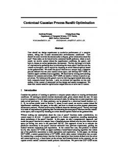
4. Experiments and Discussion This section evaluates the cumulative regret incurred by our DB-GP-UCB algorithm (5) and its scalability in the batch size empirically on two synthetic benchmark objective functions such as Branin-Hoo (Lizotte, 2008) and gSobol (González et al., 2016) (Table 3 in Appendix H) and a real-world pH field of Broom’s Barn farm (Webster & Oliver, 2007) (Fig. 3 in Appendix H) spatially distributed over a 1200 m by 680 m region discretized into a 31 ⇥ 18 grid of sampling locations. These objective functions and the real-world pH field are each modeled as a sample of a GP whose prior covariance is defined by the widelyused squared exponential kernel kxx0 , s2 exp( 0.5(x x0 )> ⇤ 2 (x x0 )) where ⇤ , diag[`1 , . . . , `d ] and s2 are its length-scale and signal variance hyperparameters, respectively. These hyperparameters together with the noise variance n2 are learned using maximum likelihood estimation (Rasmussen & Williams, 2006). The performance of our DB-GP-UCB algorithm (5) is compared with the state-of-the-art batch BO algorithms such as GP-BUCB (Desautels et al., 2014), GP-UCB-PE (Contal et al., 2013), SM-UCB (Azimi et al., 2010), q-EI (Chevalier & Ginsbourger, 2013), and BBO-LP by plugging in GP-UCB (González et al., 2016), whose implementations8 are publicly available. These batch BO algorithms are evaluated using a performance metric that measures regret incurred by a tested algorithm: PT the cumulative ⇤ et , arg maxxt 2D µ{xt } (1) f (x ) f (e x ) where x t t=1 is the recommendation of the tested algorithm after t batch evaluations. For each experiment, 5 noisy observations are randomly selected and used for initialization. This is independently repeated 64 times and we report the resulting mean cumulative regret incurred by a tested algorithm. All experiments are run on a Linux system with Intelr Xeonr E5-2670 at 2.6GHz with 96 GB memory. For our experiments, we use a fixed budget of T |DT | = 64 function evaluations and analyze the trade-off between batch size |DT | (i.e., 2, 4, 8, 16) vs. time horizon T (respectively, 32, 16, 8, 4) on the performance of the tested algorithms. This experimental setup represents a practical scenario of costly function evaluations: On one hand, when a function evaluation is computationally costly (i.e., time-consuming), it is more desirable to evaluate f for a larger batch (e.g., |DT | = 16) of inputs in parallel in each iteration t (i.e., if hardware resources permit) to reduce the total time needed (hence smaller T ). On the other hand, 8 Details on the used implementations are given in Table 4 in Appendix I. We implemented DB-GP-UCB in MATLAB to exploit the GPML toolbox (Rasmussen & Williams, 2006).

when a function evaluation is economically costly, one may be willing to instead invest more time (hence larger T ) to evaluate f for a smaller batch (e.g., |DT | = 2) of inputs in each iteration t in return for a higher frequency of information and consequently a more adaptive BO to achieve potentially better performance. In some settings, both factors may be equally important, that is, moderate values of |DT | and T are desired. To the best of our knowledge, such a form of empirical analysis does not seem to be available in the batch BO literature. Fig. 2 shows results9 of the cumulative regret incurred by the tested algorithms to analyze their trade-off between batch size |DT | (i.e., 2, 4, 8, 16) vs. time horizon T (respectively, 32, 16, 8, 4) using a fixed budget of T |DT | = 64 function evaluations for the Branin-Hoo function (left column), gSobol function (middle column), and real-world pH field (right column). Our DB-GP-UCB algorithm uses the configurations of [N, B] = [4, 2], [8, 5], [16, 10] in the experiments with batch size |DT | = 4, 8, 16, respectively; in the case of |DT | = 2, we use our batch variant of GPUCB (2) which is equivalent to DB-GP-UCB when N = 1. It can be observed that DB-GP-UCB achieves lower cumulative regret than GP-BUCB, GP-UCB-PE, SM-UCB, and BBO-LP in all experiments (with the only exception being the gSobol function for the smallest batch size of |DT | = 2 where BBO-LP performs slightly better) since DB-GPUCB can jointly optimize a batch of inputs while GPBUCB, GP-UCB-PE, SM-UCB, and BBO-LP are greedy batch algorithms that select the inputs of a batch one at time. Note that as the real-world pH field is not as wellbehaved as the synthetic benchmark functions (see Fig. 3 in Appendix H), the estimate of the Lipschitz constant by BBO-LP is potentially worse, hence likely degrading its performance. Furthermore, DB-GP-UCB can scale to a much larger batch size of 16 than the other batch BO algorithms that also jointly optimize the batch of inputs, which include q-EI, PPES (Shah & Ghahramani, 2015) and q-KG (Wu & Frazier, 2016): Results of q-EI are not available for |DT | 4 as they require a prohibitively huge computational effort to be obtained10 while PPES can only operate with a small batch size of up to 3 for the Branin-Hoo function and up to 4 for other functions, as reported in (Shah & Ghahramani, 2015), and q-KG can only operate with a small batch size of 4 for all tested functions (including the Branin-Hoo function and four others), as reported in (Wu & Frazier, 2016). The scalability of DB-GP-UCB is attributed to our proposed Markov approximation of our 9 Error bars are omitted in Fig. 2 to preserve the readability of the graphs. A replication of the graphs in Fig. 2 including standard error bars is provided in Appendix K. 10 In the experiments of González et al. (2016), q-EI can reach a batch size of up to 10 but performs much worse than GP-BUCB, which is likely due to a considerable downsampling of possible batches available for selection in each iteration.

Distributed Batch Gaussian Process Optimization DB-GP-UCB GP-UCB-PE GP-BUCB SM-UCB BBO-LP qEI

6 5

Regret

4

4 3

2

2

1

1

3

20

2

5

0

30

10

20

30

3

DB-GP-UCB GP-UCB-PE GP-BUCB SM-UCB BBO-LP

2.5

10

0 10

batch BO algorithms.

15

5

3

0

Regret

6

10

20

30

8

5. Conclusion

6

This paper develops a novel distributed batch GP-UCB (DB-GP-UCB) algorithm for performing batch BO of highly complex, costly-to-evaluate, noisy black-box objective functions. In contrast to greedy batch BO algorithms (Azimi et al., 2010; Contal et al., 2013; Desautels et al., 2014; González et al., 2016), our DB-GP-UCB algorithm can jointly optimize a batch of inputs and, unlike (Chevalier & Ginsbourger, 2013; Shah & Ghahramani, 2015; Wu & Frazier, 2016), still preserve scalability in the batch size. To realize this, we generalize GP-UCB (Srinivas et al., 2010) to a new batch variant amenable to a Markov approximation, which can then be naturally formulated as a multi-agent DCOP in order to fully exploit the efficiency of its state-of-the-art solvers such as max-sum (Farinelli et al., 2008; Rogers et al., 2011) for achieving linear time in the batch size. Our proposed DB-GP-UCB algorithm offers practitioners the flexibility to trade off between the approximation quality and time efficiency by varying the Markov order. We provide a theoretical guarantee for the convergence rate of our DB-GP-UCB algorithm via bounds on its cumulative regret. Empirical evaluation on synthetic benchmark objective functions and a real-world pH field shows that our DB-GP-UCB algorithm can achieve lower cumulative regret than the greedy batch BO algorithms such as GP-BUCB, GP-UCB-PE, SM-UCB, and BBO-LP, and scale to larger batch sizes than the other batch BO algorithms that also jointly optimize the batch of inputs, which include q-EI, PPES, and q-KG. For future work, we plan to generalize DB-GP-UCB (a) to the nonmyopic context by appealing to existing literature on nonmyopic BO (Ling et al., 2016) and active learning (Cao et al., 2013; Hoang et al., 2014a;b; Low et al., 2008; 2009; 2011; 2014a) as well as (b) to be performed by a multi-robot team to find hotspots in environmental sensing/monitoring by seeking inspiration from existing literature on multi-robot active sensing/learning (Chen et al., 2012; 2013b; 2015; Low et al., 2012; Ouyang et al., 2014). For applications with a huge budget of function evaluations, we like to couple DB-GP-UCB with the use of parallel/distributed sparse GP models (Chen et al., 2013a; Hoang et al., 2016; Low et al., 2015) to represent the belief of the unknown objective function efficiently.

2.5 2

1.5

1.5

1

1

0.5

0.5

4

2

0

0 5

5

10

15

1.5

5

10

15

4

3 1

1 2 0.5

0.5

1

0

0 2

1

4

6

0

8


0.8

Regret

0

15


1.5

Regret

10

2

4

6

8

2

0.8

2

0.6

1.5

0.4

1

0.2

0.5

4

6

8

0.6 0.4 0.2 0

0 1

2

3

T

Branin-Hoo

4

0 1

2

3

4

We have also investigated and analyzed the trade-off between approximation quality and time efficiency of our DPGP-UCB algorithm and reported the results in Appendix J due to lack of space. To summarize, it can be observed from our results that the approximation quality improves near-linearly with an increasing Markov order B at the expense of higher computational cost (i.e., exponential in B).

1

2

3

T

T

gSobol

pH field

4

Figure 2. Cumulative regret incurred by tested algorithms with varying batch sizes |DT | = 2, 4, 8, 16 (rows from top to bottom) using a fixed budget of T |DT | = 64 function evaluations for the Branin-Hoo function, gSobol function, and real-world pH field.

batch variant of GP-UCB (2) (Section 3), which can then be naturally formulated as a multi-agent DCOP (5) in order to fully exploit the efficiency of one of its state-of-the-art solvers called max-sum (Farinelli et al., 2008). In the experiments with the largest batch size of |DT | = 16, we have reduced the number of iterations in max-sum to less than 5 without waiting for convergence to preserve the efficiency of DB-GP-UCB, thus sacrificing its BO performance. Nevertheless, DB-GP-UCB can still outperform the other tested


Acknowledgements This research is supported by Singapore Ministry of Education Academic Research Fund Tier 2, MOE2016-T2-2-156. Erik A. Daxberger would like to thank Volker Tresp for his advice throughout this research project.

References Anderson, B. S., Moore, A. W., and Cohn, D. A nonparametric approach to noisy and costly optimization. In Proc. ICML, 2000. Asif, A. and Moura, J. M. F. Block matrices with L-blockbanded inverse: Inversion algorithms. IEEE Trans. Signal Processing, 53(2):630–642, 2005. Azimi, J., Fern, A., and Fern, X. Z. Batch Bayesian optimization via simulation matching. In Proc. NIPS, pp. 109–117, 2010. Brochu, E., Cora, V. M., and de Freitas, N. A tutorial on Bayesian optimization of expensive cost functions, with application to active user modeling and hierarchical reinforcement learning. arXiv:1012.2599, 2010. Cao, N., Low, K. H., and Dolan, J. M. Multi-robot informative path planning for active sensing of environmental phenomena: A tale of two algorithms. In Proc. AAMAS, pp. 7–14, 2013. Chapman, A., Rogers, A., Jennings, N. R., and Leslie, D. A unifying framework for iterative approximate bestresponse algorithms for distributed constraint optimisation problems. The Knowledge Engineering Review, 26 (4):411–444, 2011. Chen, J., Low, K. H., Tan, C. K.-Y., Oran, A., Jaillet, P., Dolan, J. M., and Sukhatme, G. S. Decentralized data fusion and active sensing with mobile sensors for modeling and predicting spatiotemporal traffic phenomena. In Proc. UAI, pp. 163–173, 2012. Chen, J., Cao, N., Low, K. H., Ouyang, R., Tan, C. K.-Y., and Jaillet, P. Parallel Gaussian process regression with low-rank covariance matrix approximations. In Proc. UAI, pp. 152–161, 2013a. Chen, J., Low, K. H., and Tan, C. K.-Y. Gaussian processbased decentralized data fusion and active sensing for mobility-on-demand system. In Proc. RSS, 2013b. Chen, J., Low, K. H., Jaillet, P., and Yao, Y. Gaussian process decentralized data fusion and active sensing for spatiotemporal traffic modeling and prediction in mobilityon-demand systems. IEEE Trans. Autom. Sci. Eng., 12: 901–921, 2015.

Chevalier, C. and Ginsbourger, D. Fast computation of the multi-points expected improvement with applications in batch selection. In Proc. 7th International Conference on Learning and Intelligent Optimization, pp. 59–69, 2013. Contal, E., Buffoni, D., Robicquet, A., and Vayatis, N. Parallel Gaussian process optimization with upper confidence bound and pure exploration. In Proc. ECML/PKDD, pp. 225–240, 2013. Contal, E., Perchet, V., and Vayatis, N. Gaussian process optimization with mutual information. In Proc. ICML, pp. 253–261, 2014. Csató, L. and Opper, M. Sparse online Gaussian processes. Neural Computation, 14(3):641–669, 2002. Desautels, T., Krause, A., and Burdick, J. W. Parallelizing exploration-exploitation tradeoffs in Gaussian process bandit optimization. JMLR, 15:4053–4103, 2014. Farinelli, A., Rogers, A., Petcu, A., and Jennings, N. R. Decentralised coordination of low-power embedded devices using the max-sum algorithm. In Proc. AAMAS, pp. 639–646, 2008. González, J., Dai, Z., Hennig, P., and Lawrence, N. D. Batch Bayesian optimization via local penalization. In Proc. AISTATS, 2016. Hennig, P. and Schuler, C. J. Entropy search for information-efficient global optimization. JMLR, 13: 1809–1837, 2012. Hensman, J., Fusi, N., and Lawrence, N. D. Gaussian processes for big data. In Proc. UAI, 2013. Hernández-Lobato, J. M., Hoffman, M. W., and Ghahramani, Z. Predictive entropy search for efficient global optimization of black-box functions. In Proc. NIPS, pp. 918–926, 2014. Hoang, Q. M., Hoang, T. N., and Low, K. H. A generalized stochastic variational Bayesian hyperparameter learning framework for sparse spectrum Gaussian process regression. In Proc. AAAI, pp. 2007–2014, 2017. Hoang, T. N., Low, K. H., Jaillet, P., and Kankanhalli, M. Active learning is planning: Nonmyopic ✏-Bayesoptimal active learning of Gaussian processes. In Proc. ECML/PKDD Nectar Track, pp. 494–498, 2014a. Hoang, T. N., Low, K. H., Jaillet, P., and Kankanhalli, M. Nonmyopic ✏-Bayes-optimal active learning of Gaussian processes. In Proc. ICML, pp. 739–747, 2014b. Hoang, T. N., Hoang, Q. M., and Low, K. H. A unifying framework of anytime sparse Gaussian process regression models with stochastic variational inference for big data. In Proc. ICML, pp. 569–578, 2015.


Hoang, T. N., Hoang, Q. M., and Low, K. H. A distributed variational inference framework for unifying parallel sparse Gaussian process regression models. In Proc. ICML, pp. 382–391, 2016.

Ouyang, R., Low, K. H., Chen, J., and Jaillet, P. Multirobot active sensing of non-stationary Gaussian processbased environmental phenomena. In Proc. AAMAS, pp. 573–580, 2014.

Kathuria, T., Deshpande, A., and Kohli, P. Batched Gaussian process bandit optimization via determinantal point processes. In Proc. NIPS, pp. 4206–4214, 2016.

Rasmussen, C. E. and Williams, C. K. I. Gaussian Processes for Machine Learning. MIT Press, 2006.

Leite, A. R., Enembreck, F., and Barthès, J.-P. A. Distributed constraint optimization problems: Review and perspectives. Expert Systems with Applications, 41(11): 5139–5157, 2014. Ling, C. K., Low, K. H., and Jaillet, P. Gaussian process planning with Lipschitz continuous reward functions: Towards unifying Bayesian optimization, active learning, and beyond. In Proc. AAAI, pp. 1860–1866, 2016. Lizotte, D. J. Practical Bayesian optimization. Ph.D. Thesis, University of Alberta, 2008. Low, K. H., Dolan, J. M., and Khosla, P. Adaptive multirobot wide-area exploration and mapping. In Proc. AAMAS, pp. 23–30, 2008. Low, K. H., Dolan, J. M., and Khosla, P. Informationtheoretic approach to efficient adaptive path planning for mobile robotic environmental sensing. In Proc. ICAPS, pp. 233–240, 2009. Low, K. H., Dolan, J. M., and Khosla, P. Active Markov information-theoretic path planning for robotic environmental sensing. In Proc. AAMAS, pp. 753–760, 2011. Low, K. H., Chen, J., Dolan, J. M., Chien, S., and Thompson, D. R. Decentralized active robotic exploration and mapping for probabilistic field classification in environmental sensing. In Proc. AAMAS, pp. 105–112, 2012. Low, K. H., Chen, J., Hoang, T. N., Xu, N., and Jaillet, P. Recent advances in scaling up Gaussian process predictive models for large spatiotemporal data. In Ravela, S. and Sandu, A. (eds.), Dynamic Data-Driven Environmental Systems Science: First International Conference, DyDESS 2014, pp. 167–181. LNCS 8964, Springer International Publishing, 2014a. ¨ ul, E. B. Low, K. H., Xu, N., Chen, J., Lim, K. K., and Ozg¨ Generalized online sparse Gaussian processes with application to persistent mobile robot localization. In Proc. ECML/PKDD Nectar Track, pp. 499–503, 2014b. Low, K. H., Yu, J., Chen, J., and Jaillet, P. Parallel Gaussian process regression for big data: Low-rank representation meets Markov approximation. In Proc. AAAI, pp. 2821– 2827, 2015.

Rogers, A., Farinelli, A., Stranders, R., and Jennings, N. R. Bounded approximate decentralised coordination via the max-sum algorithm. AIJ, 175(2):730–759, 2011. Shah, A. and Ghahramani, Z. Parallel predictive entropy search for batch global optimization of expensive objective functions. In Proc. NIPS, pp. 3312–3320, 2015. Shahriari, B., Swersky, K., Wang, Z., Adams, R. P., and de Freitas, N. Taking the human out of the loop: A review of Bayesian optimization. Proceedings of the IEEE, 104 (1):148–175, 2016. Shewry, M. C. and Wynn, H. P. Maximum entropy sampling. J. Applied Statistics, 14(2):165–170, 1987. Srinivas, N., Krause, A., Kakade, S., and Seeger, M. Gaussian process optimization in the bandit setting: No regret and experimental design. In Proc. ICML, pp. 1015– 1022, 2010. Villemonteix, J., Vazquez, E., and Walter, E. An informational approach to the global optimization of expensiveto-evaluate functions. J. Glob. Optim., 44(4):509–534, 2009. Webster, R. and Oliver, M. Geostatistics for Environmental Scientists. John Wiley & Sons, Inc., 2007. Wu, J. and Frazier, P. The parallel knowledge gradient method for batch Bayesian optimization. In Proc. NIPS, pp. 3126–3134, 2016. Xu, N., Low, K. H., Chen, J., Lim, K. K., and Ozgul, E. B. GP-Localize: Persistent mobile robot localization using online sparse Gaussian process observation model. In Proc. AAAI, pp. 2585–2592, 2014.


A. Derivation of I[fD ; yDt |yD1:t-1 ] Term in (2) By the definition of conditional mutual information,

I[fD ; yDt |yD1:t-1 ] = H[yDt |yD1:t-1 ] H[yDt |fD , yD1:t-1 ] = H[yDt |yD1:t-1 ] H[yDt |fDt ] = 0.5|Dt | log(2⇡e) + 0.5 log | n2 I + ⌃Dt Dt | = 0.5 log(| n2 I + ⌃Dt Dt || n2 I| 1 ) = 0.5 log(| n2 I + ⌃Dt Dt || n 2 I|) = 0.5 log |I + n 2 ⌃Dt Dt |

0.5|Dt | log(2⇡e)

0.5 log |

2 n I|

where the third equality is due to the definition of Gaussian entropy, that is, H[yDt |yD1:t-1 ] , 0.5|Dt | log(2⇡e) + 0.5 log | n2 I +⌃Dt Dt | and H[yDt |fDt ] , 0.5|Dt | log(2⇡e)+0.5 log | n2 I|, the latter of which follows from ✏ = yx f (x) ⇠ N (0, n2 ) for all x 2 Dt and hence p(yDt |fDt ) = N (0, n2 I).

B. Proof of Proposition 1

log | = = = = =

D t Dt |

1

log | Dt Dt | log |U > U | log |U > ||U | log |U |2 N Y 2 log |Unn | n=1

N X

=

2

=

n=1 N X

= =

n=1 N X n=1 N X n=1

= =

N X

n=1 N X n=1

log |Unn |

log |Unn |2 > log |Unn ||Unn | > log |Unn Unn |

> log |Unn Unn | > log |(Unn Unn )

1

1

|

where the first, third, fourth, eighth, ninth, and last equalities follow from the properties of the determinant, the second 1 equality is due to the Cholesky factorization of Dt Dt , and the fifth equality follows from the property that the determinant QN of an upper triangular block matrix is a product of determinants of its diagonal blocks (i.e., |U | = n=1 |Unn |).


C. Proof of Proposition 4 From the definition of DKL (

Dt Dt ,

Dt Dt ),

DKL ( ⇣Dt Dt , Dt Dt ) 1 = 0.5 tr( Dt Dt Dt Dt ) log | ⇣ ⌘ 1 = 0.5 log | Dt Dt Dt Dt |

Dt Dt

1 Dt Dt |

|Dt |

⌘

= 0.5 log | Dt Dt | + log | Dt Dt | = 0.5 log | Dt Dt | 0.5 log | Dt Dt | = ˜I[fD ; yDt |yD1:t-1 ] I[fD ; yDt |yD1:t-1 ] . The second equality is due to tr(

Dt Dt

1 Dt Dt )

= tr(

1 D t Dt )

Dt Dt

= tr(I) = |Dt |, which follows from the observations 1 Dt Dt

that the blocks within the B-block bands of Dt Dt and Dt Dt coincide and follows that DKL ( Dt Dt , Dt Dt ) = ˜I[fD ; yDt |yD1:t-1 ] I[fD ; yDt |yD1:t-1 ] |Dt | ⇣ ⌘ X = 0.5 log | Dt Dt | 0.5 log 1 + n 2 ⌃b{xb1}{xb } b=1

 0.5 log =

|Dt | X

Y

1+

n

x2Dt

0.5 log 1 +

2

n

b=1



|Dt | X

⇣

0.5 log 1 +

b=1

 exp(2C)

|Dt | X

n

2

⌃{x}{x}

2

|Dt | X

X b=1

⇣

n

⇣

2

⌃b{xb1}{xb }

1)

0.5 log 1 +

= (exp(2C)

1) I[fD ; yDt |yD1:t-1 ] .

n

2

⇣ 0.5 log 1 +

⇣ 0.5 log 1 +

exp(2C)⌃b{xb1}{xb }

= (exp(2C)

b=1

|Dt | X

b=1 |Dt |

⌃{xb }{xb }

0.5 log 1 +

b=1

!

⌘ ⌘

|Dt | X b=1

|Dt | X b=1

⌃b{xb1}{xb }

⌘

n

n

2

2

is B-block-banded (Proposition 3). It

⌃b{xb1}{xb }

⌃b{xb1}{xb }

⇣ 0.5 log 1 + ⇣ 0.5 log 1 +

n

n

⌘

⌘

2

⌃b{xb1}{xb }

2

⌃b{xb1}{xb }

⌘ ⌘

The second and last equalities are due to Lemma 4 in Appendix F and ⌃b{xb1}{xb } is defined in Definition 1 in Appendix F. The first inequality is due to Hadamard’s inequality and the observation that the blocks within the B-block bands of Dt Dt and Dt Dt (and thus their diagonal elements) coincide. The second inequality is due to Lemma 2 in Appendix F. The third inequality is due to Bernoulli’s inequality. Remark. The first inequality can also be interpreted as bounding the approximated information gain for an arbitrary Dt Dt by the approximated information gain for the Dt Dt with the highest possible degree of our proposed Markov approximation, i.e., for N = |Dt | and B = 0. In this case, all inputs of the batch are assumed to have conditionally independent corresponding outputs such that the determinant of the approximated matrix reduces toQthe product of its diagonal elements which are equal to the diagonal elements of the original matrix. Thus, | Dt Dt |  x2Dt 1 + n 2 ⌃{x}{x} which interestingly coincides with Hadamard’s inequality. Note that we only consider B 1 for our proposed algorithm (Proposition 2) since the case of B = 0 entails an issue similar to that discussed at the beginning of Section 3 of selecting the same input |Dt | times within a batch.

D. Minimal KL Distance of Approximated Matrix For the approximation quality of Dt Dt (4), the following result shows that the Kullback-Leibler (KL) distance of Dt Dt from Dt Dt is the least among all |Dt | ⇥ |Dt | matrices with a B-block-banded inverse: Proposition 5. Let KL distance DKL ( , e ) , 0.5(tr( e 1 ) log | e 1 | |Dt |) between two |Dt | ⇥ |Dt | symmetric positive definite matrices and e measure the error of approximating with e . Then, DKL ( D D , D D )  t

t

t

t


DKL ( Proof.

Dt Dt ,

e ) for any matrix e with a B-block-banded inverse.

DKL ( ⇣Dt Dt ,

= 0.5 tr( ⇣ = 0.5 tr( ⇣ = 0.5 tr( = DKL (

Dt Dt ) + DKL ( Dt Dt , 1 Dt Dt Dt Dt ) log | Dt Dt Dt Dt Dt Dt

Dt Dt

e e

, e) .

1

)

1

)

The second equality is due to tr(

e)

⌘ ⇣ |Dt | + 0.5 tr( ⌘ log | Dt Dt | log | e 1 | |Dt | ⌘ log | Dt Dt e 1 | |Dt | Dt Dt

1 D t Dt )

1 D t Dt |

= tr(

Dt Dt

1 Dt Dt )

D t Dt

e

1

) log |

Dt Dt

e

1

| |Dt |

⌘

= tr(I) = |Dt |, which follows from the observa1

tions that the blocks within the B-block bands of Dt Dt and Dt Dt coincide and Dt Dt is B-block-banded (Proposition 3). The third equality follows from the first observation above and the definition that e 1 is B-block-banded. Since DKL ( Dt Dt , e ) 0, DKL ( Dt Dt , Dt Dt )  DKL ( Dt Dt , e ).

E. Pseudocode for DB-GP-UCB

Algorithm 1 DB-GP-UCB Input: Objective function f , input domain D, batch size |Dt |, time horizon T , prior mean mx and kernel kxx0 , approximation parameters B and N for t = 1, . . . , T do 8 q > < 1> µDt + ↵t I[fD ; yDt |y (2) if B = N 1 , D 1:t-1 ] Select acquisition function a(Dt ) , q P N > > : B | 0.5↵t log | Dtn Dtn |Dtn (5) otherwise n=1 1 µDtn + Select batch Dt , arg maxDt ⇢D a(Dt ) Query batch Dt to obtain yDt , (f (x) + ✏)> x2D t end for e , arg maxx2D µ{x} Output: Recommendation x

F. Proof of Theorem 1

We first define a different notion of posterior variance: Definition 1 (Updated Posterior Variance). Let Dt , {x1 , . . . , x|Dt | } be the batch selected in iteration t. Assume an arbitrary ordering of the inputs in Dt . Then, for 0  b 1 < |Dt |, ⌃b{xb1}{xb } is defined as the updated posterior variance at input xb that is obtained by applying (1) conditioned on the previous inputs in the batch Dtb 1 , {x1 , . . . , xb 1 }. Note that performing this update is possible without querying Dtb 1 since ⌃b{xb1}{xb } is independent of the outputs yDb 1 . For b

1 = 0, ⌃b{xb1}{xb } reduces to ⌃{xb }{xb } .

t

The following lemmas are necessary for proving our main result here: P1 Lemma 1. Let 2 (0, 1) be given and t , 2 log(|D|⇡t / ) where t=1 ⇡t 1 = 1 and ⇡t > 0. Then, ⇣ ⌘ Pr 8x 2 D 8t 2 N |f (x) µ{x} |  t1/2 ⌃1/2 1 . {x}{x}

Lemma 1Pabove corresponds to Lemma 5.1 in (Srinivas et al., 2010); see its proof therein. For example, ⇡t = t2 ⇡ 2 /6 > 0 1 satisfies t=1 ⇡t 1 = 1.

Lemma 2. For f sampled from a known GP prior with known noise variance n2 , the ratio of ⌃{xb }{xb } to ⌃b{xb1}{xb } for all xb 2 Dt is bounded by ⇣ ⌘ ⌃{xb }{xb } = exp 2 I[f ; y |y ]  exp(2C) b 1 D1:t-1 {xb } Dt ⌃b{xb1}{xb }


where ⌃b{xb1}{xb } and Dtb

1

are previously defined in Definition 1, and for all x 2 D and t 2 N, C

I[f{x} ; yDb 1 |yD1:t-1 ] t

is a suitable constant. Lemma 2 above is a combination of Proposition 1 and equation 9 in (Desautels et al., 2014); see their proofs therein. The only difference is that we equivalently bound the ratio of variances instead of the ratio of standard deviations, thus leading to an additional factor of 2 in the argument of exp. Remark. Since the upper bound exp(2C) will appear in our regret bounds, we need to choose C suitably. A straightforward choice C , |Dt | 1 = maxA⇢D,|A||Dt | 1 I[fD ; yA ] maxA⇢D,|A||Dt | 1 I[fD ; yA |yD1:t-1 ] I[fD ; yDb 1 |yD1:t-1 ] t I[f{x} ; yDb 1 |yD1:t-1 ] (see equations 11, 12, and 13 in (Desautels et al., 2014)) is unfortunately unsatisfying from the t perspective of asymptotic scaling since it grows at least as ⌦(log |Dt |), thus implying that exp(2C) grows at least linearly in |Dt | and yielding a regret bound that is also at least linear in |Dt |. The work of Desautels et al. (2014) shows that when initializing an algorithm suitably, one can obtain a constant C independent of the batch size |Dt |. Refer to Section 4 in (Desautels et al., 2014) for a more detailed discussion. Lemma 3. For all t 2 N and xb 2 Dt ,

where C0 , 2/ log(1 +

n

2

⇣ ⌃b{xb1}{xb }  0.5C0 log 1 +

n

2

⌃b{xb1}{xb }

⌘

).

Lemma 3 above corresponds to an intermediate step of Lemma 5.4 in (Srinivas et al., 2010); see its proof therein. Lemma 4. The information gain for a batch Dt chosen in any iteration t can be expressed in terms of the updated posterior variances of the individual inputs xb 2 Dt , b 2 {1, . . . , |Dt |} of the batch Dt . That is, for all t 2 N, I[fD ; yDt |yD1:t-1 ] = 0.5

|Dt | X b=1

⇣ log 1 +

n

2

⌘ ⌃b{xb1}{xb } .

Lemma 4 above corresponds to Lemma 5.3 in (Srinivas et al., 2010) (the only difference being that we equivalently sum over 1, . . . , |Dt | instead of 1, . . . , T ); see its proof therein.

Lemma 5. Let 2 (0, 1) be given, C0 , 2/ log(1 + n 2 ), and ↵t , C0 |Dt | exp(2C) t where t and exp(2C) are previously defined in Lemmas 1 and 2, respectively. Then, ! X p Pr 8Dt ⇢ D 8t 2 N |f (x) µ{x} |  ↵t I[fD ; yDt |yD1:t-1 ] 1 . x2Dt

Proof. For all Dt ⇢ D and t 2 N,

X

x2Dt

= 

t

t

⌃{x}{x}

|Dt | X b=1 |Dt |

t

X b=1

⌃{xb }{xb } exp(2C) ⌃b{xb1}{xb }

 0.5C0 exp(2C)

t

|Dt | X b=1

⇣ log 1 +

= C0 exp(2C) t I[fD ; yDt |yD1:t-1 ] = |Dt | 1 ↵t I[fD ; yDt |yD1:t-1 ]

n

2

⌃b{xb1}{xb }

⌘


where the first inequality is due to Lemma 2, the second inequality is due to Lemma 3, and the second equality is due to Lemma 4. Thus, X

1/2

t

x2Dt

1/2

⌃{x}{x}

s X  |Dt |

t ⌃{x}{x}

x2Dt



p ↵t I[fD ; yDt |yD1:t-1 ]

where the first inequality is due to the Cauchy-Schwarz inequality. It follows that X

p Pr 8Dt ⇢ D 8t 2 N |f (x) µ{x} |  ↵t I[fD ; yDt |yD1:t-1 ] x2Dt ! X X 1/2 1/2 Pr 8Dt ⇢ D 8t 2 N |f (x) µ{x} |  t ⌃{x}{x} x2D x2D t t⌘ ⇣ Pr 8x 2 D 8t 2 N |f (x) µ{x} |  t1/2 ⌃1/2 {x}{x} 1

!

where the first two inequalities are due to the property that for logical propositions A and B, [A =) B] =) [Pr(A)  Pr(B)], and the last inequality is due to Lemma 1. Lemma 6. Let ⌫t for all t 2 N,

˜I[fD ; yD |yD ] t 1:t-1

I[fD ; yDt |yD1:t-1 ] be an upper bound on the approximation error of

N q X 0.5 log |

n=1

B | Dtn Dtn |Dtn

p



Dt D t .

Then,

N (I[fD ; yDt |yD1:t-1 ] + ⌫t ) .

Proof. N q X

n=1 v

0.5 log |

B | Dtn Dtn |Dtn

u N u X  tN 0.5 log |

B | Dtn Dtn |Dtn

q n=1 = N ˜I[fD ; yDt |yD1:t-1 ] q = N (I[fD ; yDt |yD1:t-1 ] + ˜I[fD ; yDt |yD1:t-1 ] p  N (I[fD ; yDt |yD1:t-1 ] + ⌫t )

I[fD ; yDt |yD1:t-1 ])

where the first inequality is due to the Cauchy-Schwarz inequality. Lemma 7. Let t 2 N be given. If X

x2Dt

|f (x)

P for all Dt ⇢ D, then x2D t rx q 2 |Dt | 2 ↵t N (I[fD ; yDt |yD1:t-1 ] + ⌫t ).

µ{x} |  

p

(6)

↵t I[fD ; yDt |yD1:t-1 ]

q 2 ↵t N (I[fD ; yDt |yD1:t-1 ] + ⌫t )

and

minx2Dt rx




Proof.

X

rx

x2D t X

= =

x2D Xt

x2D t 0

@

(f (x⇤ )

f (x))

f (x⇤ )

X

X

x2D t

= = 

q q q

f (x) 1

x2D t

µ{x} +

q

↵t N (I[fD ; yDt |yD1:t-1 ] + ⌫t )A 0

↵t N (I[fD ; yDt |yD1:t-1 ] + ⌫t ) + @

X

x2D t

X

↵t N (I[fD ; yDt |yD1:t-1 ] + ⌫t ) +

x2D q t

↵t N (I[fD ; yDt |yD1:t-1 ] + ⌫t ) + q = 2 ↵t N (I[fD ; yDt |yD1:t-1 ] + ⌫t ) .

µ{x}

µ{x}

X

x2D t

X

x2D t

f (x)

f (x) 1

(7)

f (x)A

↵t N (I[fD ; yDt |yD1:t-1 ] + ⌫t )

The first equality in (7) is by definition (Section 2). The first inequality in (7) is due to X

f (x⇤ )

x2DX t

=

f (x)

x2Dt⇤

  =

X

x2Dt⇤

X

x2Dt⇤

X

x2Dt⇤

  

X

x2Dt⇤

X

x2D t

X

x2D t

µ{x} + µ{x} +

q ↵t I[fD ; yDt⇤ |yD1:t-1 ] q ↵t ˜I[fD ; yDt⇤ |yD1:t-1 ]

v u N u X µ{x} + t↵t 0.5 log | n=1

N p Xq µ{x} + ↵t 0.5 log |

µ{x} + µ{x} +

p

↵t

n=1 N q X

n=1

0.5 log |

(8)

⇤ D ⇤ |D ⇤B | Dtn tn tn

⇤ D ⇤ |D ⇤B | Dtn tn tn

B

D tn D tn |D tn

q ↵t N (I[fD ; yDt |yD1:t-1 ] + ⌫t )

|

where, in (8), the first inequality is due to (6), the second inequality is due to Proposition 4 (see the paragraph after this qP PN p N proposition in particular), the third inequality is due to the simple observation that n=1 an n=1 an , the fourth ⇤ inequality follows from the definition of Dt in (5) and, with a slight abuse of notation, Dt is defined as a batch of |Dt | inputs x⇤ , and the last inequality is due to Lemma 6. The last inequality in (7) follows from (6) and an argument equivalent to the one in (8) (i.e., by substituting Dt⇤ by Dt ). From (7),

min rx 

x2D t

q 1 X rx  2 |Dt | |Dt | x2D t

2↵

t

N (I[fD ; yDt |yD1:t-1 ] + ⌫t ) .


Main Proof. RT0 T X X = rx t=1 x2D t

T q X  2 ↵t N (I[fD ; yDt |yD1:t-1 ] + ⌫t ) t=1 v u T u X  2t T ↵t N (I[fD ; yDt |yD1:t-1 ] + ⌫t )

v t=1 u u  2t T ↵ N T

T X t=1

I[fD ; yDt |yD1:t-1 ] +

q = 2 T ↵T N I[fD ; yD1:T ] + ⌫¯T p 2 q T ↵T N ( T + ⌫¯T ) = C2 T |DT | exp(2C) T N ( T + ⌫¯T )

T X

⌫t

t=1

!

holds with probability 1 where the first equality is by definition (Section 2), the first inequality follows from Lemmas 5 and 7, the second inequality is due to the Cauchy-Schwarz inequality, the third inequality is due to the non-decreasing ↵ Pt Twith increasing t, the second equality follows from the chain rule for mutual information and the definition of ⌫¯T , t=1 ⌫t , the fourth inequality is by definition (Theorem 1), and the third equality is due to the definition of ↵t in Lemma 5, |D1 | = . . . = |DT | and the definition that C2 , 4C0 = 8/ log(1 + n 2 ). Analogous reasoning leads to the result that

RT =

T X t=1

min rx  2

x2D t

holds with probability 1

q T |DT |

2↵

T

N(

T

+ ⌫¯T ) =

q C2 T |DT |

1

exp(2C)

T

N(

T

+ ⌫¯T )

, where the first equality is by definition (Section 2).

G. Comparison of Regret Bounds

Table 1. Bounds on RT ( TP, 2 log(|D|T 2 ⇡ 2 /(6 )), C1 , 4/ log(1 + n 2 ), C2 , 2C1 , C3 , 9C1 ). Note that |DT | = 1 in T T for GP-UCB and HDPP , 1)-DPP with kernel K (see t=1 H(DP P (Kt )) with H(DP P (K)) denoting the entropy of a (|Dt | (Kathuria et al., 2016) for details on their proposed kernels). Also, note that for DB-GP-UCB andp GB-BUCB, we assume the use of the initialization strategy proposed by Desautels et al. (2014); otherwise, the factor C 0 is replaced by exp(2C).

BO Algorithm

DB-GP-UCB (5) GP-UCB-PE (Contal et al., 2013) GP-BUCB (Desautels et al., 2014) GP-UCB (Srinivas et al., 2010) UCB-DPP-SAMPLE (Kathuria et al., 2016)

Bound on RT p C C2 T |DT | 1 T N ( T + ⌫¯T ) p C1 T |DT | 1 T T p C 0 C2 T |DT | 1 T |DT | T p C2 T T T 0

p 2C3 T |DT |

T

[

T

HDPP + |DT | log(|D|)]

Distributed Batch Gaussian Process Optimization Table 2. Bounds on maximum mutual information T (Srinivas et al., 2010; Kathuria et al., 2016) and values of C 0 (Desautels et al., 2014) for different commonly-used kernels (↵ , d(d + 1)/(2⌫ + d(d + 1))  1 with ⌫ being the Matérn parameter).

Kernel

Linear RBF Matérn

T

C0

d log(T |DT |) d (log(T |DT |)) (T |DT |)↵ log(T |DT |)

exp(2/e) exp((2d/e)d ) e

H. Synthetic Benchmark Objective Functions and Real-World pH Field

Table 3. Synthetic benchmark objective functions.

Name

Function

Branin-Hoo

f (x) = a(x2 bx21 + cx1 r)2 + s(1 t) cos(x1 ) + s where a = 1, b = 5.1/(4⇡ 2 ), c = 5/⇡, r = 6, s = 10, and t = 1/(8⇡). d Y |4xi

2| + ai 1 + ai i=1 where d = 2 and ai = 1 for i = 1, . . . , d. P2 f (x) = 1 r(xi )) i=1 (g(xi )

gSobol

f (x) =

Mixture of cosines

where g(xi ) = (1.6xi

D

[ 5, 15]2

[ 5, 5]2

[ 1, 1]2

0.5)2 and r(xi ) = 0.3 cos(3⇡(1.6xi

0.5)).

18 8.5

16 8

14

12

7.5

10 7

8 6.5

6

4

6

2 5.5

5

10

15

20

25

Figure 3. Real-world pH field of Broom’s Barn farm (Webster & Oliver, 2007).

30


I. Details on the Implementations of Batch BO Algorithms Table 4. Details on the available implementations of the batch BO algorithms for comparison with DB-GP-UCB in our experiments.

BO Algorithm

Language

URL of Source Code

GP-BUCB SM-UCB GP-UCB-PE q-EI BBO-LP

MATLAB MATLAB MATLAB R Python

http://www.gatsby.ucl.ac.uk/˜tdesautels/ http://www.gatsby.ucl.ac.uk/˜tdesautels/ http://econtal.perso.math.cnrs.fr/software/ http://cran.r-project.org/web/packages/DiceOptim/ http://sheffieldml.github.io/GPyOpt/

J. Analysis of the Trade-Off between the Approximation Quality vs. Time Efficiency of DB-GP-UCB We now analyze the trade-off between the approximation quality vs. time efficiency of DB-GP-UCB by varying the Markov order B and number N of functions in DCOP. The mixture of cosines function (Anderson et al., 2000) is used as the objective function f and modeled as a sample of a GP. A large batch size |DT | = 16 is used as it allows us to compare a multitude of different configurations of [N, B] 2 {[16, 14], [16, 12], . . . , [16, 0], [8, 6], [8, 4], [8, 2], [8, 0], [4, 2], [4, 0], [2, 0]}. The acquisition function in our batch variant of GP-UCB (2) is used as the performance metric to evaluate the approximation quality of the batch DT (i.e., by plugging DT into (2) to compute the value of the acquisition function) produced by our DB-GP-UCB algorithm (5) for each configuration of [N, B]. Fig. 4 (top) shows results of the normalized values of the acquisition function in (2) achieved by plugging in the batch DT produced by DP-GP-UCB (5) for different configurations of [N, B] such that the optimal value of (2) (i.e., achieved in the case of N = 1) is normalized to 1. Fig. 4 (bottom) shows the corresponding time complexity of DP-GP-UCB plotted in log|D| -scale, thus displaying the values of (B + 1)|DT |/N . It can be observed that the approximation quality improves near-linearly with an increasing Markov order B at the expense of higher computational cost (i.e., exponential in B). Value of acq. function

1.02 1 0.98 0.96 0.94 0.92 B=N-1 N=1 [16,14] [16,12] [16,10] [16,8] [16,6] [16,4] [16,2] [16,0]

[8,6]

[8,4]

[8,2]

[8,0]

[4,2]

[4,0]

[2,0]

B=N-1 N=1 [16,14] [16,12] [16,10] [16,8] [16,6] [16,4] [16,2] [16,0]

[8,6]

[8,4]

[8,2]

[8,0]

[4,2]

[4,0]

[2,0]

Time complexity

20 15 10 5 0

Configuration of [N,B]

Figure 4. (Top) Mean of the normalized value of the acquisition function in (2) (over 64 experiments of randomly selected noisy observations of size 5) achieved by plugging in the batch DT (of size 16) produced by our DP-GP-UCB algorithm (5) for different configurations of [N, B] (including the case of N = 1 yielding the optimal value of (2)); note that the horizontal line is set at the optimal baseline of y = 1 for easy comparison and the y-axis starts at y = 0.915. (Bottom) Time complexity of DP-GP-UCB for different configurations of [N, B] plotted in log|D| -scale.


K. Replication of Regret Graphs including Error Bars 6

6 DB-GP-UCB GP-UCB-PE GP-BUCB SM-UCB BBO-LP qEI

4

Regret

Regret

4

5

3

12 10

3

2

2

1

1

0

0

DB-GP-UCB GP-UCB-PE GP-BUCB SM-UCB BBO-LP qEI

14

Regret

5

16 DB-GP-UCB GP-UCB-PE GP-BUCB SM-UCB BBO-LP qEI

8 6 4

5

10

15

20

25

30

2 5

10

15

T 3

25

0

30

1

0.5

0.5

4

6

8

10

12

14

2

4

6

8

10

12

14

1.2

2

4

6

8

10

12

14

16

6

7

8

3.5

4

T 4


1.2 1


3.5 3 2.5

0.8

0.8

Regret

Regret

1

Regret

3

0

16

1.4

1.4

30

4

T


25

1

T 1.6

20

2

0

16

5

1.5

1

2

15


6

Regret

2

1.5

0

10

7 DB-GP-UCB GP-UCB-PE GP-BUCB SM-UCB BBO-LP

2.5

Regret

2

5

T

3 DB-GP-UCB GP-UCB-PE GP-BUCB SM-UCB BBO-LP

2.5

Regret

20

T

0.6

0.6

2 1.5

0.4

0.4 0.2

0.2

0

0

1

2

3

4

5

6

7

8

1 0.5 1

2

3

4

T

5

6

7

0

8

0.9

0.7

2

3

4

5

T 2

0.8 DB-GP-UCB GP-UCB-PE GP-BUCB SM-UCB BBO-LP

0.8

1

T


0.7 0.6


1.5

0.5

0.5

Regret

Regret

Regret

0.6

0.4

1

0.4 0.3

0.3

0.1

0.5

0.2

0.2 1

1.5

2

2.5

T

Branin-Hoo

3

3.5

4

0.1

1

1.5

2

2.5

T

gSobol

3

3.5

4

0

1

1.5

2

2.5

3

T

pH field

Figure 5. Cumulative regret incurred by tested algorithms with varying batch sizes |DT | = 2, 4, 8, 16 (rows from top to bottom) using a fixed budget of T |DT | = 64 function evaluations for the Branin-Hoo function, gSobol function, and real-world pH field. The error bars denote the standard error.