High Dimensional Bayesian Optimization with Elastic Gaussian Process

High Dimensional Bayesian Optimization with Elastic Gaussian Process

Santu Rana * 1 Cheng Li * 1 Sunil Gupta 1 Vu Nguyen 1 Svetha Venkatesh 1

Abstract Bayesian optimization is an efficient way to optimize expensive black-box functions such as designing a new product with highest quality or tuning hyperparameter of a machine learning algorithm. However, it has a serious limitation when the parameter space is high-dimensional as Bayesian optimization crucially depends on solving a global optimization of a surrogate utility function in the same sized dimensions. The surrogate utility function, known commonly as acquisition function is a continuous function but can be extremely sharp at high dimension - having only a few peaks marooned in a large terrain of almost flat surface. Global optimization algorithms such as DIRECT are infeasible at higher dimensions and gradient-dependent methods cannot move if initialized in the flat terrain. We propose an algorithm that enables local gradient-dependent algorithms to move through the flat terrain by using a sequence of gross-tofiner Gaussian process priors on the objective function as we leverage two underlying facts a) there exists a large enough length-scales for which the acquisition function can be made to have a significant gradient at any location in the parameter space, and b) the extrema of the consecutive acquisition functions are close although they are different only due to a small difference in the length-scales. Theoretical guarantees are provided and experiments clearly demonstrate the utility of the proposed method on both benchmark test functions and real-world case studies.

1. Introduction Bayesian optimization method has established itself as an efficient way to optimize black-box functions (Jones et al., *

Equal contribution 1 Centre for Pattern Recognition and Data Analytics (PRaDA), Deakin University, Australia. Correspondence to: Santu Rana . Proceedings of the 34 th International Conference on Machine Learning, Sydney, Australia, PMLR 70, 2017. Copyright 2017 by the author(s).

1998) which are also expensive to evaluate. Examples include experimental design to optimize the quality of a physical product (Brochu et al., 2010) or hyperparameter tuning of machine learning algorithms (Bardenet et al., 2013). In both cases the response functions are unknown and each evaluation of either making the product to test the quality or training a model from large data can be time-consuming. Likewise, it has found applications in a variety of domains including computer vision (Denil et al., 2012) and sensor set selection (Garnett et al., 2010). Bayesian optimization is a sequential procedure where a probabilistic form of the unknown function is maintained using a Gaussian process (GP). A GP is specified by a mean function and a covariance function. A popular choice of covariance function is the squared exponential kernel (Rasmussen and Williams, 2005). A crucial parameter of the kernel is the length-scale which dictates prior belief about the smoothness of the objective function. The posterior of a Gaussian process is analytically tractable and is used to estimate both the mean and the variance of the estimation at unobserved locations. Next, a cheap surrogate function is built that seeks the location where lies the highest possibility of obtaining a higher response. The possibility is expressed through a variety of acquisition functions which trade-off exploitation of the predicted best mean and exploration around high predicted variance. Typical acquisition functions include Expected Improvement (EI) (Mockus, 1994) and GP-UCB (Srinivas et al., 2010). Acquisition functions are continuous functions, yet they may be extremely sharp functions at higher dimensions, especially when the size of observed data is small. Generally, they have some peaks and a large area of mostly flat surface. For this reason, the global optimization of high-dimensional acquisition functions is hard and can be prohibitively expensive. This makes it difficult to scale Bayesian optimization to high dimensions. Generic global optimization algorithms such as DIRECT (Jones et al., 1993) or simplex-based methods such as Nelder-Mead (Olsson and Nelson, 1975) or genetic algorithm based methods (Runarsson and Yao, 2005; Beyer and Schwefel, 2002) perform reasonably when the dimension is low, but at higher dimensions they can become extremely inefficient and actually become infeasible within the practical limitation of resource and time. Multi-start based method start


Limited work has addressed the issue of highdimensionality in Bayesian optimization. Nearly all the existing work assumes that the objective function only depends on a limited number of “active” features (Chen et al., 2012; Wang et al., 2013; Djolonga et al., 2013). For example, Wang et al. (2013) projected the high-dimensional space into a low-dimensional subspace by random embedding and then optimized the acquisition function in a low-dimensional subspace assuming that many dimensions are correlated. This assumption seems too restrictive in real applications (Kandasamy et al., 2015; Li et al., 2017). The Add-GP-UCB model (Kandasamy et al., 2015) allows the objective function to vary along the entire feature domain. The objective function is assumed to be the sum of a set of low-dimensional functions with disjoint feature dimensions. Thus the optimization of acquisition function is performed in the low-dimensional space. Li et al. (2016a) further generalized the AddGP-UCB by eliminating an axis-aligned representation. However, none of them are not applicable if the underlying function does not have assumed structure, that is, if the dimensions are not correlated or if the function is not decomposable in some predefined forms. Thus efficient Bayesian optimization for high dimensional functions is still an open problem. To address that we propose an efficient algorithm to optimize the acquisition function in high dimension without requiring any assumption on the structure of the underlying function. We recall a key characteristic of the acquisition function that they are mostly flat functions with only a few peaks. Gradients on the large mostly flat surfaces of the high-dimensional acquisition functions would be close to zero. Thus gradient-dependent methods would fail to work since a random initialization would most likely fall in the large flat region. However, we theoretically prove that for a location where the gradient is currently insignificant it is possible to find a large enough kernel length-scale which when used to build a new GP can make the derivative of the new acquisition function becomes significant. Different locations may need different length-scales above which the derivative at that location becomes significant. We prove it for both the Expected Improvement (EI) and Upper Confidence Bound (UCB) acquisition functions. Next, we theoretically prove that the difference in the acquisition func-

GaussianPDF(10d)

1

kernel length scale = 0.5 kernel length scale = 0.3 kernel length scale = 0.1

0.8

Simple Regret

from multiple initializations to achieve local maxima and then choose the best one. However, the multi-start method may not be able to find the non-flat portion of the acquisition function by random search. A related discussion for high dimensional Bayesian optimization concerns with the usefulness of Gaussian process for high dimensional modeling. Fortunately, Srinivas et al. (2010) showed that Gaussian process (GP) can handle “curse of dimensionality” to a good extent.

0.6

0.4

0.2 0

20

40

60

80

100

Iteration

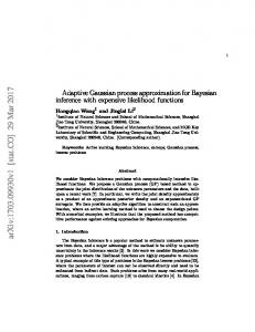
Figure 1. Simple regret as a function of iteration for an unnormalized GaussianPDF function with maximum of 1 in 10 dimension using three different length scales for SE kernel. Average and standard errors for 20 trials with different initializations is reported.

tions is smooth with respect to the change in length-scales, which implies that the extremums of the consecutive acquisition functions are close if the difference in the lengthscales is small. Based on these two observations we build a novel optimization algorithm for acquisition functions. In the first part of our algorithm we search for a large enough length-scale for which a randomly selected location in the domain starts to have significant gradients. Next, we gradually reduce the length scale to move from a gross to a finer function approximation, controlling this transition by slowly reducing the length-scale of the Gaussian process kernel. We solve a sequence of local optimization problems wherein we begin with a very gross approximation of the function and then the extrema of this approximation is used as the initial point for the optimization of the next approximation which is a little bit finer. Following this sequence we reach to the extrema of the acquisition function for the Gaussian process with the target length-scale. The target length-scale is either pre-specified by the user or estimated for some covariance functions. It may seem to the reader that the problem can be avoided if a large length scale is chosen for the original GP model itself, however, as it shows in Figure 1 the right length-scale actually lies at a smaller value, especially for high dimensional functions. Since in our algorithm we use Gaussian processes with large to small length-scales akin to fitting an elastic function, we denote our method as Elastic Gaussian Process (EGP) method. We note that EGP is a meta-algorithm that enables a gradient-dependent local optimization algorithm to perform by removing the problem associated with flat surface. Newton’s gradient based method is used as a local optimization tool for our algorithm. It is to be noted that our algorithm EGP can easily be converted to pursue a global solution by employing multiple starts with different random initializations. We demonstrate our algorithm on two synthetic examples and two real-world applications involving one of training


cascaded classifier and the other involving optimization of an alloy based on thermodynamic simulation. We compare with the the state-of-the-art additive model (Kandasamy et al., 2015), high dimensional optimization using random embedding (Wang et al., 2013), a vanilla multi-start method and 2x random search. All the methods are given equal computational budget to have a fair comparison. In all experiments our proposed method outperforms the baselines. In summary, our main contributions are:

where k = [k(xt+1 , x1 ) · · · k(xt+1 , xt )]T and K(x, x) = K(x1:t , x1:t ). We simplify the problem by using m(x1:t ) = 0. The predictive distribution of ft+1 can be represented by 2 ft+1 | f1:t ∼ N (µt+1 (xt+1 | x1:t , f1:t ), σt+1 (xt+1 | x1:t , f1:t )) (2.3)

with µt+1 (.) = kT K−1 f1:t T −1 k(xt+1 , xt+1 ) − k K k.

and

2 σt+1 (.)

=

2.2. Bayesian Optimization • Proposal of a new method to handle high dimensional Bayesian optimization without any assumptions about the underlying structure in the objective function; • Derivation of theoretical guarantees that underpins our proposed algorithm; • Validation on both synthetic and real-world applications to demonstrate the usefulness of our method.

2. Background 2.1. Gaussian Process We briefly review Gaussian process (Rasmussen and Williams, 2005) here. Gaussian process (GP) is a distribution over functions specified by its mean m(.) and covariance kernel function k(., .). Give a set of observations x1:t , the probability of any finite set of f is Gaussian f (x1:t ) ∼ N (m(x1:t ), K(x1:t , x1:t )) where f (x1:t ) is a vector of response values of K(x1:t , x1:t ) is a covariance matrix presented by  k(x1 , x1 ) · · · k(x1 , xt )  .. .. .. K(x1:t , x1:t ) =  . . . k(xt , x1 )

···

(2.1) x1:t and    (2.2)

k(xt , xt )

where k is a kernel function. If the observations are contaminated with noise, K should include the noise variance. The choice of the kernel depends on prior beliefs about smoothness properties of the objective function. A popular kernel function is the squared exponential (SE) function, which is defined as 1 k(xi , xj ) = exp − 2 ||xi − xj ||2 2l

A traditional optimization problem is to find the maximum or minimum of a function f (x) over a compact domain X . In real applications such as hyperparameter tuning for a machine learning model or experiments involving making of physical products, f (x) is unknown in advance and expensive to evaluate. Bayesian optimization (BO) is a powerful tool to optimize such expensive black-box functions. A common method to model the unknown function is using a Gaussian process as a prior. The posterior is maintained based on observations and allows prediction for expected function values at unseen locations (Eq.2.3). A acquisition function a(x | x1:t , f1:t ) is constructed to guide the search for the optimum. Some examples about acquisition functions include Expected Improvement (EI) and UCB (Srinivas et al., 2010). The EI-based acquisition function is to compute the expected improvement with respect to the current maximum f (x+ ). The improvement function is written as I(x) = max{0, ft+1 (x) − f (x+ )} ft+1 (x) is Gaussian distributed with the mean µ(x) and variance σ 2 (x), as per the predictive distribution of GP (2.3). Thus the expected improvement is the expectation over these Gaussian variables. In closed form (Mockus et al., 1978; Jones et al., 1998), ( (µ(x) − f (x+ ))Φ(Z) + σ(x)φ(Z) σ(x) > 0 EI(x) = 0 σ(x) = 0 (2.4) (x+ ) where Z = µ(x)−f . Φ(Z) and φ(Z) are the CDF and σ(x) PDF of standard normal distribution. The UCB (Srinivas et al., 2010) acquisition function is defined as UCB(x) = µ(x) + νσ(x) (2.5)

where the kernel length-scale l reflects the smoothness of the objective function.

where ν is a sequence of increasing positive numbers.

The predictive distribution of GP is tractable analytically. For a new point xt+1 , the joint probability distribution of the known values f1:t = f (x1:t ) and the predicted function value ft+1 is given by K(x, x) k f1:t m(x1:t ) ∼N , ft+1 m(xt+1 ) kT k(xt+1 , xt+1 )

In each iteration of Bayesian optimization, the most promising xt+1 is found by maximizing the acquisition function and then yt+1 is evaluated. The new observation is augmented to update the GP and in turn is used to construct a new acquisition function. These steps are repeated till a satisfactory outcome is reached or the iteration budget is exhausted.


2.2.1. O PTIMIZATION OF ACQUISITION F UNCTIONS

3. High-dimensional Bayesian Optimization with Elastic Gaussian Process We would like to employ Bayesian optimization to solve a high-dimensional maximization problem maxx∈X f (x) in a compact subset X ⊆ R. To model f (x), we use a Gaussian process with zero mean as a prior and the SE kernel as the covariance function with a target length-scale lτ . The target length-scale can be set by the user or can be separately inferred by using the maximum likelihood-based estimation method (Snoek et al., 2012). The SE kernel although a simple kernel, is versatile and popular. Hence we choose to use it in our framework. Acquisition functions, such as EI (Mockus, 1994) and UCB (Srinivas et al., 2010), depend on the predictive mean µ(x) and variance σ 2 (x) of GP µ(x) σ 2 (x)

= kT K−1 y =

1 − kT K−1 k

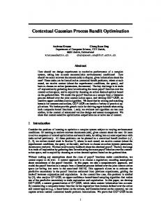
Hence, the acquisition function is also associated with the GP kernel length-scale l and we denote it as a(x | D1:t , l). The core task of Bayesian optimization is to find the most promising point xt+1 for the next function evaluation by globally maximizing acquisition function. Figure 2 serves as an inspired example for our approach. We plot the acquisition function for different length-scales. As can be seen when the length-scale is low, some portions of the parameter space are flat. This is especially remark-

5 x*l=0.4 4

xinit l=0.35

x*l=0.35

l =0.4 l =0.35

3

l =0.3 l =0.25 l =0.2 l =0.15 l =0.1

a(x)

In Bayesian optimization, the objective function is expensive to evaluate while the acquisition function is tractable analytically. Our task is to maximize the acquisition function a(x | D1:t ) over a compact region or with constraints. Global optimization heuristics are often used to find the extremum of a function. The gradient-based and derivativefree approaches are two main types. Gradients for the EI acquisition function can be computed as in (Frean and Boyle, 2008). DIRECT (Jones et al., 1993) is a popular choice to globally optimize the acquisition function. It is a deterministic and derivative-free algorithm which divides the search space into smaller and smaller hyperrectangles and leverages the Lipschitizian-continuity of the acquisition function. However. it takes time exponential to dimension and becomes practically infeasible beyond 10 dimensions. The multi-start gradient based approach is potentially attractive in high dimension but it mostly fails in high-dimensional scenario as a random initialization may not be able to escape from the large flat region that acquisition functions generally have. Our proposed method utilizes properties of the acquisition function to derive a meta-algorithm that enables the gradient-based optimizer to move even when initialized in a seemingly flat region.

2 1 0 0

0.2

0.4

0.6

0.8

1

x

Figure 2. The illustration for the elastic Gaussian process (EGP) at one dimension. The acquisition function presents different terrains with varied kernel length-scales l. The optimal points at l = 0.35 and l = 0.4 are close. The optimal point x∗l=0.35 can be ∗ achieved if the initial point (xinit l=0.35 ) is the point xl=0.4 .

able in high-dimensional problems. For example, the acquisition function with length-scale 0.1 is extremely flat. However when the length-scale is above 0.2, the acquisition functions starts to have significant gradients. Additionally, we also show that the optimal solutions for different length-scales are close. We construct our method based on the above observations. Specifically in Lemma 1 we theoretically guarantee that it is possible to find a large enough length-scale for which the derivative of the acquisition function becomes non-insignificant at any location in the domain. Proof for both the Expected Improvement (EI) and Upper Confidence Bound (UCB) based acquisition functions are derived. Relying on this guarantee, we search for a large enough length-scale for which a randomly selected location in the domain starts to have significant gradients. Next in Lemma 2, we theoretically guarantee that the difference in the acquisition function is smooth with respect to the change in length-scale. This implies that the extrema of the consecutive acquisition functions are close but different only due to a small difference in the length-scales. The details of these lemmas are provided later. However, we can now conceive that an algorithm to overcome flat region can be constructed by first finding a large enough length-scale to solve for the optima at that length-scale and then gradually reduce the length-scale and solve a sequence of local optimization problems wherein the optimum of a larger length-scale is used as the initialization for the optimization of the acquisition function based on the Gaussian process with a smaller length-scale. This is continued till the optimum at the target length-scale lτ is reached. We denote our method as Elastic GP (EGP) method. The whole proposed algorithms are presented in Alg.1 and Alg. 2.


Algorithm 1 High Dimensional Bayesian Optimization with Elastic Gaussian Process 1: for t = 1, 2 · · · do 2: Sample the next point xt+1 ←argmaxxt+1∈X a(x | D1:t , l) using Alg. 2 3: Evaluate the value yt+1 4: Augment the data D1:t+1 = {D1:t , {xt+1 , yt+1 }} 5: Update the kernel matrix K 6: end for 3.1. Theoretical Analysis In the first step of our algorithm (seen in Step 1 of Alg.2) , we want to show that gradient of the acquisition functions becomes significant beyond a certain l so that our algorithm can find an optimal solution compared to any start point.

∂a(x)

Lemma 1. ∃l :

∂x ≥ ε for lτ ≤ l ≤ lmax . 2

Proof. The Lemma can be proved if we prove that ∂a(x) ∂xi ≥ ε, ∀i. We consider both forms: UCB and EI. • For the UCB acquisition function (Eq. 2.5), the partial derivative of UCB can be written as ∂a(x) ∂xi

= =

The

∂kT ∂xi

∂µ(x) ∂σ(x) +ν ∂xi ∂xi ∂kT −1 ν ∂kT −1 K y+ (− K k) ∂xi σ(x) ∂xi

is dependent on the form of the covariance func∂cov(x,x )

j tion: it is 1 × t matrix whose (1, j)th element is . ∂xi For the SE kernel ∂cov(x, xj ) ||x − xj ||2 (xi − xji ) = exp − − ∂xi 2l2 l2 dji (3.1) = − 2 cov(x, xj ) l

where dji = xi − xji . To simplify the proof, we assume that we have the worst case that only one observation x0 exists and thus ∂a(x) ∂xi y0 ∂cov(x, x0 ) vcov(x, x0 ) ∂cov(x, x0 ) = −p 2 ∂xi ∂xi 1 − cov (x, x0 ) d0i d0i vcov(x, x0 ) cov(x, x0 ) = − 2 cov(x, x0 )y0 + p 2 l 1 − cov (x, x0 ) l2 ! vcov 2 (x, x0 ) d0i = 2 p − cov(x, x0 )y0 (3.2) l 1 − cov 2 (x, x0 )

Algorithm 2 Optimizing acquistion function using EGP Input: a random start point xinit ∈ χ, the length-scale interval 4l, l = lτ . 1: Step 1: 2: while l ≤ lmax do 3: Sample x∗ ← argmaxx∗ ∈X a(x | D1:t , l) starting

with xinit ; 4: if ||xinit − x∗ || = 0 then 5: l = l + 4l 6: else 7: xinit = x∗ , break; 8: end if 9: end while 10: Step 2: 11: while l ≥ lτ do 12: l = l − 4l 13: Sample x∗ ← argmaxx∗ ∈X a(x | D1:t , l) starting

with xinit ; 14: if ||xinit − x∗ || = 0 then 15: 4l=4l/2 16: else 17: xinit = x∗ 18: end if 19: end while

Output: the optimal point xt+1 = x∗ to be used in Alg.1

The cov(x, x0 ) is a small value due to ||x − x0 || 0 and then the first term in the fourth line of the Eq.(3.2) can be ignored compared to its second term. Therefore we have ∂a(x) ∂xi

d0i cov(x, x0 )y0 l2 d0i y0 ||x − x0 ||2 = − 2 exp − l 2l2 = −

(3.3)

We rewrite it as α ∂a(x) α1 2 ∂xi = l2 exp − l2 where α1 = |d0i y0 | and α2 = ||x − x0 ||2 /2. 2 α2 To have ∂a(x) ≥ εl ∂xi ≥ ε, the equation exp − l2 α1 must hold for a l between lτ ≤ l ≤ lmax . In fact, we can find a l to hold the inequality since exp − αl22 is a decreasing 2 function with the range (0, 1] whilst εl α1 is an increasing function with the range (0, +∞) by considering lτ can approach to 0 and lmax can approach to infinity in theory. Therefore Lemma 1 has been proved for the UCB acquisition function.


• For the EI acquisition function (Eq. 2.4), the partial derivative can be written as ∂a(x) ∂xi

=

where Z =

[ZΦ(Z) + φ(Z)]

µ(x)−f (x+ ) σ(x)

and

∂σ(x) =− ∂xi ∂Z = ∂xi

∂σ(x) ∂Z + σ(x)Φ(Z) ∂xi ∂xi

∂kT −1 K k /σ(x) ∂xi

∂kT −1 ∂σ(x) K y−Z ∂xi ∂xi

/σ(x)

therefore, ∂kT −1 ∂kT −1 K k /σ(x)+Φ(Z) K y ∂xi ∂xi (3.4) We substitute Eq.(3.1) into Eq. (3.4) and make the similar assumption within the proof at the UCB acquisition function. The Eq. (3.4) then becomes as ∂a(x) = −φ(Z) ∂xi

For the UCB, we compute the derivative of g(x, l) with respect to l based on Eq.(3.3) ||x − x0 ||2 ∂g(xi , l) 2d0i y0 exp − = ∂l l3 2l2 d0i y0 ||x − x0 ||2 ||x − x0 ||2 + 2 exp − l 2l2 l3

∂a(x) ∂xi y0 Φ(Z)∂cov(x, x0 ) φ(Z)cov(x, x0 ) ∂cov(x, x0 ) = −p ∂xi ∂xi 1 − cov 2 (x, x0 ) ! 2 φ(Z)cov (x, x0 ) d0i = 2 p − cov(x, xj )y0 Φ(Z) l 1 − cov 2 (x, x0 ) Since φ(Z) lies 0-1, we can ignore the first term. The equation above is further written as ||x − x0 ||2 µ(x) − f (x+ ) ∂a(x) d0i y Φ( ) = − 2 exp − 0 ∂xi l 2l2 σ(x) As l increasing, µ(x) becomes smaller and σ(x) becomes larger and then Φ(·) → 1. The equation above becomes similar with Eq.(3.3). Therefore Lemma 1 is proved for EI. In the second step of our algorithm (seen in Step 2 of Alg.2), our purpose is to find 4l which makes the start point of the local optimizer move to a finer region. We need to show that ∂a(x) ∂a(x) − ≤ ε, f or 4l < δ ∂xi l=l∗ ∂xi l=l∗ +4l 1:t ,l) being smooth. The folIt is directly related to ∂a(x|D ∂x lowing lemma guarantees that.

Lemma 2. g(x, l) is a smooth function with respect to l, 1:t ,l) where g(x, l) = ∂a(x|D . ∂x

i ,l) Apparently, ∂g(x is continuous in the domain of l. ∂l Therefore, g(x, l) is a smooth function with respect to l. The similar proof can be done for EI.

4. Experiments We evaluate our method on three different benchmark test functions and two real-world applications including training cascaded classifiers and for alloy composition optimization. We use low memory BFGS implementation in NLopt (Johnson, 2014) as the local optimization algorithm, and a variant of DIRECT (GN DIRECT L) for global optimization1 . Our comparators are: • Global optimization using DIRECT (Global) • Multi-start local optimization (Multi-start) • High-dimensional Bayesian optimization via additive models (Kandasamy et al., 2015) (Add-d0 , where d0 is the dimensionality in each group) • Bayesian optimization using random embedding (Wang et al., 2013) (REMBO-d0 , where d0 is the projected dimensionality) • Best of 2 x Random search, which has shown competitiveness over many algorithms(Li et al., 2016b). Global optimization with DIRECT is used only at dimension d ≤ 10 as it consistently returns erroneous results at higher dimension. For the additive model variables are divided into a set of additive clusters by maximizing the marginal likelihood (Kandasamy et al., 2015). In all experiments, we use EI as the acquisition function and the SE kernel as the covariance function. The search bounds are rescaled √ to [0, 1]. We use the target length-scale lτ = 0.1, lmax = d and 4lmin = 10−5 . In Figure 1 we plot the simple regret vs iteration for three different choices of scale l = 0.1, 0.3 and 0.5. Out of them l = 0.1 provides the fastest convergence, justifying our choice for the lengthscale. In our experience any smaller length-scale slows down the convergence and surprisingly, in most of the cases lτ = 0.1 turns out to be a good choice. The number of initial observations are set at d + 1. All the algorithms are 1

The code is available on request.


1

1 0.5

0.5 0

0.8

1.5

0

10

20

30

40

50

0

60

0.8

0.6 0.4 Global Multistart EGP Best(2xRandom Search)

0.2

0

10

20

30

40

50

0

60

Iteration

Iteration

(a) Hertmann6d(Topt = 6ms)

(b) Hertmann6d(Topt = 60ms)

GaussianPDF(10d)

1

Simple Regret

1.5

GaussianPDF(10d)

1

Global Multistart EGP Best(2xRandom Search)

2

Simple Regret

Simple Regret

2

Hartmann6(6d)

2.5


Simple Regret

Hartmann6(6d)

3 2.5

0

20

40

60

0.6 0.4 Global Multistart EGP Best(2xRandom Search)

0.2

80

0

100

0

20

Iteration

40

60

80

100

Iteration

(c) Gaussian10d(Topt = 10ms) (d) Gaussian10d(Topt = 100ms)

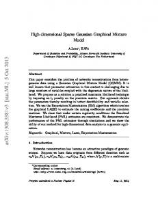
Figure 3. Simple regret as a function of Bayesian optimization iteration. Optimization time Topt shown is for each iteration. Both mean (line) and the standard errors are reported for 20 trials with random initializations.

3

Simple Regret

10


2.5

Rosenbrock(20d)

1.5 1

0

50

6 4

100

150

200

0

0.8 0.6 0.4 EGP Multistart Best(2xRandom Search)

0.2

0

50

Iteration

100

150

GaussianPDF(50d)

1 0.9

2

0.5

GaussianPDF(20d)

1

Multistart Best(2xRandom Search) EGP

8

2

0

#10 5

Simple Regret

Rosenbrock(10d)

Simple Regret

#10 5

Simple Regret

3.5

200

Iteration

0

0

50

100

0.8 0.7 0.6 0.5 0.4 0.3

150

200

Iteration

(a) Rosenbrock10d(Topt = 1sec) (b) Rosenbrock20d(Topt = 2sec) (c) Gaussian20d(Topt = 2sec)

0.2

Multistart EGP Best(2xRandom Search) 100

200

300

400

500

Iteration

(d) Gaussian50d(Topt = 5sec)

Figure 4. Simple regret as a function of Bayesian optimization iteration. Optimization time Topt has been set as 0.1 × d sec. Both mean (line) and the standard errors are reported for 20 trials with random initializations.

given the same fixed time duration per iteration (Topt ). The computer used is a Xeon Quad-core PC running at 2.6 GHz, with 16 GB of RAM. Bayesian optimization has been implemented in Matlab with mex interface to a C-based acquisition function optimizer that uses NLOPT library. We run each algorithm 20 trials with different initializations and report the average results and standard errors . 4.1. Benchmark Test Functions In this study we demonstrate the application of Bayesian optimization on three different benchmark test functions 1. Hertmann6d in [0, 1] for all dimensions. 2. Unnormalized Gaussian PDF with a maximum of 1 in [−1, 1]d for d=20 and [−0.5, 0.5]d for d=50. 3. Generalized Rosenbrock function (Picheny et al., 2013) in [−5, 10]d . We set the covariance matrix ofthe Gaussian PDF  to be A ··· 0   a block diagonal matrix Σ =  ... . . . ... , where 0 A =

h

1 0.9

0.9 1

i

···

A

. In this case, variables are partially

correlated and, therefore, the function does not admit additive decomposition with high probability. The function is further scaled such that the maximum value of the function

remains at 1 irrespective of the number of variables (dimensions). Since, for all these test functions neither the assumptions of additive decomposition based method or the assumptions of REMBO (many dimensions are correlated) are true, they perform poorly on these. Hence, we do not include them in our comparison for benchmark functions. We first demonstrate the efficiency of our EGP based optimization given limited amount of time. In Figure 3 we show how the three algorithms perform when given two different amounts of optimization time per iteration (Topt = 0.001×d and Topt = 0.01×d) on both Hertmann6 and Gaussian PDF functions. The plot shows that when Topt is small then Multi-start performs the worst, even performing lower than the 2x Random search. However, both EGP and the DIRECT perform much better and almost perform similarly. When Topt is increased then all the methods start to perform almost similarly with EGP providing slightly better performance. This demonstrates two things: a) EGP is more efficient in using time than the Multi-start, and b) EGP being gradient-based is more numerically precise than the grid-based DIRECT algorithm. In Figure 4 we demonstrate our method on both Rosenbrock and Gaussian PDF functions at high dimensions. The optimization time for all these high-dimensional optimization problem is set as Topt = 0.1×d sec. EGP clearly beats all the comparators for these benchmark test functions. Then UCB acquisition function has the similar behaviour with EI for our model although no result shown here.


d=33

0.66

d=24

0.615

0.65

d=22

0.74

0.61

0.72

0.605

0.7

4.6

0.6

Utility

0.63

AUC

4.5

AUC

0.64

AUC

d=13

4.7

4.4

0.68

0.62

4.3 EGP Best(2xRandom Search) REMBO-10 Add-10

0.61 0.6 0

50

100

150

Iteration

(a) Ionosphere

EGP Best(2xRandom Search) REMBO-10 Add-10

0.595 0.59 0

20

40

60

80

100

120

Iteration

(b) German

EGP Best(2xRandom Search) REMBO-10 Add-10

0.66 0.64 0

20

40

60

80

Iteration

(c) IJCNN1

100

EGP REMBO-5 Add-5

4.2 4.1 0

5

10

15

20

25

30

Iteration

(d) Alloy optimization

Figure 5. (a)-(c) Training AUC as a function of iteration for cascade classifier training. The number of stages in the classifier is equal to the number of features in three datasets from left to right a) Ionosphere d = 33, b) German d = 24, c) IJCNN1 d = 22. Both mean (line) and the standard errors (shaded region) are reported for 20 trials with random initializations. (d) Alloy utility value as a function of the iteration for the optimization of AA-2050 alloy system.

4.2. Training cascade classifier Here we evaluate our method by training a cascade classifier on three real datasets from UCI repository (Blake and Merz, 1998): Ionosphere, German and IJCNN1. A K-cascade classifier consists of K stages and each stage has a weak classifier, a one-level decision stump. Instances are re-weighted after each stage. Generally, independently computing the thresholds are not an optimal strategy and thus we seek to find an optimal set of thresholds by maximizing the training AUC. Features in all datesets are scaled between [0, 1]. The number of stages is set same with the number of features in the dataset. Therefore, simultaneously optimizing thresholds in multiple stages is a difficult task and thus being used as a challenging test case for highdimensional Bayesian optimization. We create the additive model with 10 dimensions per group and 10 dimensions for random embedding in REMBO. The results are plotted in Figure 5 (a)-(c). In all three cases EGP provides the best performance. REMBO performs the worst of all. Surprisingly, for IJCNN1 the Random Search turned out to be competitive to EGP. However, in the other two datasets it performs much worse than EGP. 4.3. Optimizing alloy for aeronautic applications AA-2050 is a low density high corrosion resistant alloy and is used for aerospace applications. The current alloy has been designed decades ago and is considered by our metallurgist collaborator as a prime candidate for further improvement. ThermoCalc, a software based thermodynamic simulator (Andersson et al., 2002), is used to compute the utility of a composition by looking at the occurrences of different phases at different temperatures. Some phases are beneficial for mechanical properties whereas some are not. Guided by our metallurgist partners a weighted combination of phase fractions is used as the utility function The alloy consists of 9 elements (Al, Cu, Mg, Zn, Cr, Mn, Ti, Zr, and Sc) and along with that we have 4 operational pa-

rameters that have to be optimized together. In all we have a 13-dimensional optimization problem. The result is given in Figure 5(d). Since, the simulations are expensive we run only upto 30 iterations and compare with only the additive model and the REMBO. We ran only once after starting from expert-specified starting points. Clearly, EGP is quicker in reaching better value and always remained better than both the baselines.

5. Conclusion In this paper we propose a novel algorithm for Bayesian optimization in high dimension. At high dimension the acquisition function becomes very flat on a large region of the space rendering gradient-dependent methods to fail at high dimension. We prove a) gradient can be induced by increasing the length-scales of the GP prior and b) acquisition functions which differ only due to small difference in length-scales are close. Based on these we formulate our algorithm that first finds a large enough length-scale to enable the gradient-dependent optimizer to perform, and then the gradually reduces the length-scale while also sequentially using the optimum of the larger length-scale as the initialization for the smaller. In experiments the proposed algorithm clearly performs better than the baselines on a set of test functions and two real applications of training cascade classifiers and alloy composition optimization.

Acknowledgement This work is partially funded by Australian Government through ARC and the Telstra-Deakin Centre of Excellence in Big Data and Machine Learning. Prof Venkatesh is the recipient of an ARC Australian Laureate Fellowship (FL170100006). We thank our metallurgist collaborators Dr.Thomas Dorin from Institute of Frontier Materials Deakin and his team for the alloy case study and anonymous reviewers for their valuable comments.


References Jan-Olof Andersson, Thomas Helander, Lars Höglund, Pingfang Shi, and Bo Sundman. Thermo-calc & dictra, computational tools for materials science. Calphad, 26 (2):273–312, 2002. Rémi Bardenet, Má ty a´ s Brendel, Kégl Balázs, et al. Collaborative hyperparameter tuning. In Proceedings of the 30th International Conference on Machine Learning (ICML-13), pages 199–207, 2013. Hans-Georg Beyer and Hans-Paul Schwefel. Evolution strategies–a comprehensive introduction. Natural computing, 1(1):3–52, 2002.

Kirthevasan Kandasamy, Jeff G. Schneider, and Barnabs Pczos. High Dimensional Bayesian Optimisation and Bandits via Additive Models. In ICML, 2015. C. Li, K. Kandasamy, B. Poczos, and J. Schneider. High dimensional bayesian optimization via restricted projection pursuit models. In AISTATS, pages 1–9, 2016a. Cheng Li, Sunil Kumar Gupta, Santu Rana, Svetha Venkatesh, Vu Nguyen, and Alistair Shilton. High dimensional bayesian optimisation using dropout. In The 26th International Joint Conference on Artificial Intelligence, 2017.

Catherine Blake and Christopher J Merz. {UCI} repository of machine learning databases. 1998.

L. Li, K. Jamieson, G. DeSalvo, A. Rostamizadeh, and A. Talwalkar. Hyperband:a novel bandit-based approach to hyperparameter optimization. In ArXiv e-prints, 2016b.

Eric Brochu, Vlad M. Cora, and Nando de Freitas. A tutorial on bayesian optimization of expensive cost functions, with application to active user modeling and hierarchical reinforcement learning. 2010.

J. Mockus, V. Tiesis, and A. Zilinskas. The application of bayesian methods for seeking the extremum. Towards Global Optimisation, (2):117–129, 1978.

Bo Chen, Rui Castro, and Andreas Krause. Joint optimization and variable selection of high-dimensional gaussian processes. In Proc. International Conference on Machine Learning (ICML), 2012. Misha Denil, Loris Bazzani, Hugo Larochelle, and Nando de Freitas. Learning where to attend with deep architectures for image tracking. Neural Comput., 24(8):2151– 2184, August 2012. Josip Djolonga, Andreas Krause, and Volkan Cevher. Highdimensional gaussian process bandits. In Advances in Neural Information Processing Systems, 2013. Marcus Frean and Phillip Boyle. Using Gaussian Processes to Optimize Expensive Functions, pages 258–267. Berlin, Heidelberg, 2008. Roman Garnett, Michael A Osborne, and Stephen J Roberts. Bayesian optimization for sensor set selection. In International Conference on Information Processing in Sensor Networks, 2010. Steven G. Johnson. The nlopt nonlinear-optimization package, 2014. URL http://ab-initio.mit.edu/ nlopt. D. R. Jones, C. D. Perttunen, and B. E. Stuckman. Lipschitzian optimization without the lipschitz constant. Journal of Optimization Theory and Applications, 79(1): 157–181, 1993. Donald R. Jones, Matthias Schonlau, and William J. Welch. Efficient global optimization of expensive black-box functions. Journal of Global Optimization, 13(4):455– 492, 1998. ISSN 1573-2916.

Jonas Mockus. Application of bayesian approach to numerical methods of global and stochastic optimization. Journal of Global Optimization, 4(4):347–365, 1994. Donald M Olsson and Lloyd S Nelson. The nelder-mead simplex procedure for function minimization. Technometrics, 17(1):45–51, 1975. Victor Picheny, Tobias Wagner, and David Ginsbourger. A benchmark of kriging-based infill criteria for noisy optimization. Structural and Multidisciplinary Optimization, 48(3):607–626, 2013. Carl Edward Rasmussen and Christopher K. I. Williams. Gaussian Processes for Machine Learning. The MIT Press, 2005. Thomas Philip Runarsson and Xin Yao. Search biases in constrained evolutionary optimization. Systems, Man, and Cybernetics, Part C: Applications and Reviews, IEEE Transactions on, 35(2):233–243, 2005. Jasper Snoek, Hugo Larochelle, and Ryan P Adams. Practical bayesian optimization of machine learning algorithms. In NIPS, pages 2951–2959, 2012. Niranjan Srinivas, Andreas Krause, Sham Kakade, and Matthias Seeger. Gaussian process optimization in the bandit setting: No regret and experimental design. In ICML, 2010. Ziyu Wang, Masrour Zoghi, Frank Hutter, David Matheson, and Nando De Freitas. Bayesian optimization in high dimensions via random embeddings. In IJCAI, pages 1778–1784, 2013.