Distributed Computer Vision Algorithms Through Distributed Averaging. Roberto ..... The idea of. GPCA is to fit a polynomial to the data and then recover the.
Distributed Computer Vision Algorithms Through Distributed Averaging Roberto Tron Ren´e Vidal Center for Imaging Science, Johns Hopkins University, Baltimore MD 21218, USA {tron,rvidal}@cis.jhu.edu
http://www.vision.jhu.edu
Abstract
distributed counterparts. Our basic building blocks are distributed algorithms for least squares estimation, which were first presented in [12]. We show that the same principles can be applied to all the algorithms covered in this paper. The first one, Distributed PCA, has been the subject of numerous papers (see [11] and references therein). In particular, our method can be related to [1], with the difference that [1] assumes fixed tree topology and uses local QR decompositions instead of arbitrary topologies and local weighted averages. We are not aware of any previous distributed version of GPCA [10]. Triangulation of 3-D points in a camera network has been studied in the context of camera localization [4, 8]. In those works, however, the triangulation is performed independently at each camera, while our approach uses all the images simultaneously. Prior work on pose estimation [9] averages pose estimates computed independently at each node, while we work directly with the image points. Finally, while SfM is very much related to the problem of network localization (see [8] and references therein), we are not aware of any work that uses orthographic projection model and factorization methods in a distributed setting. Overall, our main contribution is to address all the aforementioned problems under a common distributed optimization framework.
Traditional computer vision and machine learning algorithms have been largely studied in a centralized setting, where all the processing is performed at a single central location. However, a distributed approach might be more appropriate when a network with a large number of cameras is used to analyze a scene. In this paper we show how centralized algorithms based on linear algebraic operations can be made distributed by using simple distributed averages. We cover algorithms such as SVD, least squares, PCA, GPCA, 3-D point triangulation, pose estimation and affine SfM.
1. Introduction Imagine we have a large network of N cameras for analyzing a scene. A traditional solution would be to send all the images to a central node, where a large problem is set up and solved. Unfortunately, this approach is not scalable. As the number of sensors increases, the load on the central node increases, possibly exceeding the available resources. In addition, if the central node fails, the entire network becomes useless. Therefore, it might be better to use a distributed approach, where each camera in the network processes its own data, collaborates with neighboring cameras and finds a globally optimal solution to the problem using simple local computations. In this way, the computation load is shared by all the nodes (which require only a fraction of the resources) and the architecture is robust to individual node failures. We show that, for specific linear algebra operations, such as least squares and SVD (§3), the problem reduces to finding the average or the minimum of a set of values in a distributed fashion, for which well-studied algorithms are available (§2). We also show that this is the case for a few standard machine learning (§4) and computer vision (§5) algorithms.
2. Basic Distributed Algorithms In this section, we review some basic distributed algorithms. We represent the network with a connected undirected graph G = (V, E), where V = {1, . . . , N } represents the nodes and E ⊂ V × V represents the pairs (i, j) ∈ E that can communicate directly. The set of neighbors of node i is denoted as Ni = {j ∈ V : (i, j) ∈ E} and its degree as di = |Ni |. A path on the graph from node i to node j is a sequence of nodes (w0 , w1 , . . . , wm ) such that wk ∈ V, (wk , wk+1 ) ∈ E for all k and m is the length of the path. The diameter of G is defined as the maximum length of the shortest path among any pair of nodes.
Prior work. Over the past few years, many distributed algorithms for camera networks have been developed (see [8] and references therein for a review). However, different distributed approaches have been used for different problems. In this paper we propose a more general approach to directly translate specific centralized algorithms to their
2.1. Distributed Averaging Assume each node has a measurement ui ∈ R and that PN we need to compute the average u ¯ = N1 i=1 ui . 57
A first trivial approach is to aggregate averages along a spanning tree up to a designated central node. This approach is the most efficient in some situations. However, it requires selecting a central node, which could fail, and maintaining a spanning tree, which could be difficult in the case of packet losses. In addition, this kind of algorithm does not take advantage of wireless communications, where messages can be easily broadcasted from one node to its neighbors. A second alternative approach is to use an average consensus algorithm [5]. In its simplest form, each node maintains a state xi , which is initialized with a measurement xi (0) = ui . The nodes then iterate the difference equations X xi (t + 1) = xi (t) + ε (xj (t) − xi (t)), (1)
For the sake of brevity, from now on we will denote (3) and other similar quantities as A = stack({Ai }N i=1 ). Assume that we want to compute A> A (or a scaled version of it) at each node. The problem is distributed, because it involves data from all the nodes. Let us define N N 1 1 X > 1 X C = A> A = Ai Ai = Ci , (4) N N i=1 N i=1 where Ci = A> i Ai is the local correlation matrix at node i. We first remark that C is a matrix with dimension m × m, independently of the number of nodes N and of measurements n. Therefore, as the dimension of the problem grows (for instance, if we add more nodes or data at each node), the requirements for storing Ci and C at each node do not change. Our second and most important remark is that C can be computed as an average of the local Ci by using the methods of §2.1. If N is also known at each node, then the matrix A> A can be computed exactly. Moreover, since Ci is symmetric, the nodes can save transmission bandwidth by computing the Cholesky decomposition Ci = Q> i Qi and transmitting only the factor Qi , which can be represented as a lower triangular m × r matrix, where r is the rank of Ci . However, computing C in this way is advantageous only if r � n (otherwise we can just use the original data). Assume now that each node i has also a vector bi ∈ Rni and define the vector b = stack({bi }N i=1 ). Assume we want to compute A> b at each node or a scaled version of it. Similarly to before, define the cross-correlation vector
j∈Ni
where ε < (maxi {di })−1 . It can be shown that each state converges to the average of the initial values, i.e., limt→∞ xi = u ¯. The main advantages are that each node has an estimate of the mean at each iteration, that each node needs to communicate only with its neighbors and that no central coordination is needed. The price to pay is a larger number of iterations to converge. Consensus algorithm can also be adapted to situations where the topology of the network is changing or packet losses are present [13]. In all our experiments we will employ average consensus. Extensions. Both averaging algorithms mentioned above can be extended to the case of multivariate data ui ∈ Rm by applying them to each component. They can also be extended to the case where each node has multiple data points and we are interested in averaging the entire dataset. Specifi ically, assume each node i has ni measurements {uij }nj=1 P P N ni and we want to compute u ¯ = PN1 n i=1 j=1 uij . By i=1 i PN Pni ui defining ui = j=1 uij we can write u ¯ = PNN n i=1 . N i=1 i Therefore, u ¯ can be obtained by dividing the average of the ui by the average of the ni (i.e., by averaging twice).
d=
N N 1 X > 1 X 1 > A b= Ai bi = di , N N i=1 N i=1
(5)
m where di = A> i bi ∈ R is the local cross-correlation vector at node i. As before, d can be computed using distributed averaging and its dimension depends only on m. In the following, we use the distributed computation of C and d to build distributed versions of various algorithms.
2.2. Distributed computation of the minimum
3.1. Singular Value Decomposition (SVD)
Assume now that we are interested in computing u = mini ui . A simple distributed algorithm can be defined as
Assume we want to compute the compact SVD of the matrix A defined in (3), namely, A = UΣV> , where U ∈ Rn×r and V ∈ Rm×r have orthonormal columns, Σ ∈ Rr×r is diagonal with non-negative entries and r is the rank of the matrix. From (4) and the SVD of A we have 1 C = V( Σ2 )V> , (6) N which is the SVD of C. Therefore, the nodes can recover V (even without knowing N ) after a distributed average. If N is known, then the nodes can also recover Σ. While the matrices V and Σ are common to all the nodes, the matrix U must be stored similarly to A, i.e., each node computes the part of the factorization corresponding to its data as
x(0) = ui ,
xi (t + 1) =
min
j∈{Ni ∪i}
xj (t).
(2)
It is easy to show that, after at most T = diam(G) iterations, this algorithm converges to xi (T ) = u ∀i ∈ V.
3. Distributed Linear Algebra Algorithms In this section, we introduce the key insight for reducing distributed linear algebra operations to averages. Assume that each node i has a matrix Ai ∈ Rni ×m and let n = P N i=1 ni . Define the matrix � �> A> . . . A> A = A> ∈ Rn×m . (3) 1 2 N
Ui = Ai VΣ−1 . 58
(7)
3.2. Distributed Nullspace Estimation
ˆ can be computed using the algorithms in The average µ §2.1. The matrix V can be obtained from the global correla˜ > . The tion matrix C as described in §3 by setting A = Y remaining operations can all be performed locally.
Assume that, given the matrix A, we want to find the vector x0 = argmin kAxk2 . (8)
Conceptually, the proposed algorithm is just a distributed average of vectors followed by a distributed SVD. Notice that the local storage requirements do not depend on the number of nodes N . However, this approach gives a real advantage only if rank(Y) � n.
x:kxk=1
It is well known that the solution is given by x0 = v m where v m is the last column of V (completed to be a square orthonormal matrix, if necessary). Therefore, by computing the SVD of C, the desired result can be found at each node.
We tested our distributed PCA algorithm on a synthetic dataset distributed across a network with ten nodes in a ring topology. Each node has ni = 50 vectors in R2 clustered around a 1-D subspace that is slightly different for each node. Figure 1(a) shows the distribution of the vectors and the 1-D subspaces estimated using either only the local data at each node or the entire dataset. Note that each single node cannot estimate the global subspace fit alone. We used consensus to compute the distributed average and we report in Figure 1(b) the maximum subspace angles between the estimate at each node and the centralized solution after each consensus iteration. The errors converge to zero for all the nodes in the network.
3.3. Distributed Linear Least Squares Assume we want to solve a distributed system of equations Ax = b in a least squares sense, i.e., we want to find x0 = argmin kAx − bk2 .
(9)
x
The solution can be obtained by solving A> Ax0 = A> b, or equivalently, Cx0 = d, which is a m × m linear system of equations that each node can solve locally after computing the two distributed averages C and d.
4. Applications in Subspace Learning In this section we use the basic algorithms from the previous section to build distributed versions of algorithms for dimensionality reduction and subspace clustering.
20 10
4.1. Principal Component Analysis (PCA) 0
Imagine that � each node� i has a collection of ni vectors Yi = y i1 , . . . , y ini ∈ Rm×ni . Considering all we have a distributed dataset Y = �the nodes together, � Y1 , . . . , YN ∈ Rm×n . We can reduce the dimensionality of this dataset by employing PCA, which approximates the vectors using an affine subspace model given by ˆ ij + µ, ˆ ij = Vc ˆ y ij ' y
−10 −20 −30
−20
−10
0
10
20
30
(a) Data points (different colors indicate data from different nodes), subspaces estimated locally at each node (thin colored lines) and subspace estimated from the entire dataset (thick black line).
(10)
Basis angle errors (degrees)
ˆ ij ∈ Rm is the approximation of y ij , µ ˆ ∈ Rm is an where y m׈ r ˆ offset vector, V ∈ R represents an orthonormal basis for an rˆ-dimensional space in Rm and cij are the coefficients for ˆ {cij } and µ ˆ ij in this basis. PCA finds V, ˆ that minimize y the total reconstruction error in three steps: ˆ as the average of the entire dataset, i.e., µ ˆ= 1. Compute µ PN P ni 1 y and compute a centered version of ij i=1 j=1 n ˜ ij = y ij − µ ˆ (to which we collectively refer the data y ˜ as the matrix Y).
15
10
5
0
2. Compute the SVD of the centered data matrix, say ˜ = VΣU> and set V ˆ as the first rˆ columns of V. Y ˆ >y ˜ ij . 3. Compute the coefficients as cij = V
0
10
20 30 Iterations
40
50
(b) Maximum subspace angle between the subspace estimated locally at each node and the centralized solution after each iteration of consensus.
Figure 1. Results for distributed PCA.
Given this centralized solution and the algorithms presented in §3, it is easy to give a distributed version of PCA. 59
4.2. Generalized PCA (GPCA)
2. Estimate the distance of each point from its subspace ˆ> y |. as dij = |b
� Imagine now � that the measurements at each node Yi = y i1 . . . y ini are drawn from a union of K hyperplanes with m normals {bk }N k=1 ∈ R . In other words, for any point y ij there exist a k ∈ {1, . . . , K} such that b> k y ij = 0. This is the case, for instance, when the data Yi represent images of faces belonging to different individuals under varying lighting conditions. Our goal is to obtain a distributed algorithm that recovers the normals {bk } and clusters the data accordingly. Generalized PCA (GPCA) [10] is a non-iterative algorithm for solving this clustering problem. The idea of GPCA is to fit a polynomial to the data and then recover the normals from this polynomial. The main insight is to notice that any point y ij in any one of the hyperplanes satisfies 0=
K Y
> b> k y ij = pK (y ij ) = νK (y ij ) c,
ij
|bk−1 y ij |+δ
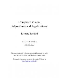
with δ being a small regularization constant. (b) Pick the normal at the point for which dij is miniˆk = b ˆˆıˆ where (ˆı, ˆ) = argmin mal, i.e., b (i,j) dij . A distributed implementation of this procedure is straightforward. All the steps use only local information, except for steps (3) and (4b), which require the computation of a global minimum. For these steps, we can use the algorithm of §2.2. Note that, the node must exchange the normal that attains the minimum in addition to the value of the minimum distance. ˆk } have been estimated, each node can Once the normals {b assign each one of its points to the closest subspace. This gives a complete, distributed version of GPCA. We tested our algorithm on a synthetic dataset distributed in a network of ten nodes connected with a ring topology. Each node generates ni = 60 data points in one of three 1-D subspaces in R2 and adds isotropic Gaussian noise whose variance is about 15% the variance of the data. Note that each node has only samples from one of the subspaces. Figure 2(a) shows an instance of the generated data together with the estimated subspaces. We report in Figure 2(b) the squared Euclidean distances between the coefficient vector c computed with a centralized algorithm and the vectors computed after each iteration of the consensus algorithm in the distributed version. All the local estimates converge to the centralized solution. In addition, the maximum angle between any normal estimated at any node and the corresponding normal from the centralized solution is 1.48 · 10−6 .
(11)
k=1
where pK is a homogeneous � polynomial in m variables with MK (m) = K+m−1 coefficients, which we denote m−1 with the vector c ∈ RMK (m) . Also, νK (y ij ) denotes the Veronese map of the vector y ij , which contains all the monomials of degree K in the entries in y ij . For the exact definition of this map, we refer the reader to [10]. The vector of coefficients c can be linearly estimated from the data. Specifically, define the matrix Ai = i stack({νK (y ij )> }nj=1 ) at each node i and the matrix A = N stack({Ai }i=1 ) . Then, according to (11), the coefficient vector c must satisfy Ac = 0, i.e., c is in the nullspace of A. In the case of noisy data points that do not exactly correspond to the subspaces, the coefficient vector can be still estimated in a least square sense as c = argminx:kxk=1 kAxk2 . In both cases, each node can estimate c using the algorithm of §3.2. Once we have obtained the coefficients c of the polynomial pK , we use polynomial differentiation to recover the normals. In the case of data lying perfectly on the hyperplanes, the gradient of pK computed at one of the points y ij gives a vector which is parallel to the normal bk of the k-th hyperplane to which that point belongs, i.e., ∇x pK (x)|x=yij ∼ bk , where b> k y ij = 0.
ij
3. For the first subspace k = 1, pick the normal at the ˆ1 = b ˆˆıˆ where (ˆı, ˆ) = point with minimum dij , i.e., b argmin(i,j) dij . 4. For the other subspaces k = 2, . . . , K, repeat d , (a) Update the distances using dij ← ˆ> ij
5. Applications in Computer Vision In this section we give distributed versions of three basic but important computer vision algorithms: point triangulation, linear pose estimation and affine Structure from Motion.
(12)
5.1. Point triangulation
When the data is noisy, we can still use this relation to get an estimate (although not perfect) of the normal at each point. Hence, all we need is to get one point in each cluster such that we can obtain the normal for each subspace. We will now explain how this can be done in a distributed way. In ˆij (with two indexes) to indicate the the following, we use b ˆk (with a sinnormal estimated at point y ij using (12) and b gle index) to indicate the normal estimated by the algorithm for the k-th subspace. The algorithm proceeds as follows: ˆij = ∇x pK (x) 1. Estimate b for each point. k ∇x pK (x)k
�> Py Pz ∈ R3 is � �> visible to all the cameras and let pi = pix piy ∈ R2 denote its image in the i-th camera. Denote as Ri ∈ SO(3) and T i ∈ R3 the rotation and translation of the i-th camera. Using the standard projective camera model [2] we have � � T i P h, λi phi = Ri (13) � Assume that a 3-D point P = Px
where λi ∈ R is the depth of the point P for camera i and the notation v h = stack(v, 1) indicates the vector v in
x=y ij
60
5.2. Linear pose estimation 2
Assume we have an object defined in a predetermined Np reference frame by NP points {P l }l=1 ∈ R3 and that this object undergoes a rigid-body transformation defined by the rotation R0 ∈ SO(3) and the translation T 0 ∈ R3 . Again, using the standard projective camera model, we have
1 0 −1
λil phil = Ri (R0 P l + T 0 ) + T i ,
−2 −4
−2
0
2
where pil ∈ R and λil are the image and the depth of the l-th point for the i-th camera. The camera poses (Ri , T i ) are assumed to be known. Our goal is to design a distributed version of the linear algorithm for recovering the pose (R0 , T o ) from the images [2]. Similar to the triangulation problem, if we multiply on the left by the cross product matrix [phil ]× , we get the relationship
4
10
10
0
10
[phil ]× (Ri (R0 P l + T 0 ) + T i ) = 0.
−10
10
y
2
−20
0
50
100
150
0
z
Squared Euclideand distances
(a) Data points (different colors indicate data from different nodes) and estimated 1-D subspaces (black lines).
10
(15)
Iterations
x z
y z x
yx z
10
Figure 2. Results for distributed GPCA.
5 y
{pi }N i=1 ,
homogeneous coordinates. Given the images one can triangulate the 3-D point P using a well known linear algorithm. First, each node i constructs � � Ai = [phi ]× Ri T i , (14)
0
−2
2
0
6
4
x
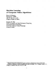
(a) Synthetic camera setup of five cameras looking at an object (a cube) composed of eight 3-D points.
where [pi ]× is the matrix representing the cross product1 . Then, the coordinates of P can be recovered using the relation AP h = 0, where A = stack({Ai }N i=1 ). In practice, in our distributed setting, each node can recover P h from the nullspace of A by applying the algorithm of §3.2 and then normalize the vector so that the last entry is equal to one. The 3-D coordinates of P are then easily extracted from P h . We tested our algorithm on a synthetic camera setup with five calibrated cameras looking at an object (Figure 3(a)). For simplicity, we assumed that all the cameras can see all the 3-D points. The images of the points in each camera have been corrupted by adding Gaussian noise with standard deviation equivalent to 15 pixels on a 1000 × 1000 image. In Figure 3(b) we show the final reconstruction together with the trajectories of the points as they are estimated during successive iterations and converge to the centralized solution. 1 [p ] v i ×
y x z y x z
−2
(b) Squared Euclidean distances between the coefficient vectors c estimated with the centralized and distributed GPCA algorithms after each iteration of consensus.
(16)
1 0 −1
1 0 −1 −2
−2
−1
0
1
(b) The centralized reconstruction of the eight 3-D points (circles) and the trajectories of each point as they are estimated after each consensus iteration. Different colors indicate data from different nodes. The squares indicate the estimates of the nodes after one iteration. The errors are magnified five times for visualization purposes.
Figure 3. Results for distributed triangulation.
= pi × v ∀v ∈ R3 and [pi ]× pi = 0
61
Rotation error [degrees]
4
2
stead of the projective camera model used previously, in this section we will consider the orthographic projection model (which can be easily generalized to the affine model [6]). Under this assumption, the image points satisfy the equation
1
pilk = Mik P l + tik .
3
0
0
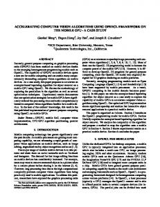
10 20 30 (a) Rotation errors (degrees).
40
When the cameras are calibrated, Mik ∈ R2×3 and tik contain the first two rows of, respectively, the rotation and translation between the camera i and the 3-D object at frame k. For ease of explanation, we define the motion matrices N i Mi = stack({Mik }K i }i=1 ), and the k=1 � ), M = stack({M � structure matrix S = P 1 · · · P NP 3×N . The goal of SfM P is to recover M and S from the image points {pilk }. Since the motion and structure of the scene can only be recovered up to a choice of the world’s reference frame, it is customary to place the origin of the world’s PNPreference frame at the center of the 3-D points, so that l=1 P l = 0. As a consequence, t can be estimated by each camera ik PNP pilk . Each camera i can then form the as tik = N1P l=1 matrices Wik ∈ R2×NP , whose NP columns are the meanP subtracted images {wilk = pilk − tik }N l=1 . Define Wi = Ki stack({Wik }k=1 ) and W = stack({Wi }N i=1 . It is easy to verify that W can be factorized as
50
Translation error
0.2 0.15 0.1 0.05 0
0
10 20 30 40 (b) Translation errors (Euclidean distance).
(17)
50
Figure 4. Results for distributed pose estimation. The plots show the errors between the pose estimated at each node after each consensus iteration and the pose estimated by the centralized algorithm.
This relation gives equations that are linear in the unknowns R0 and T 0 and can be rewritten as Dil x = dil , where the vector x = stack(vec(R0 ), T 0 ) ∈ R12 contains all the entries of R0 and T 0 , while Dil and dil contain the coefficients of the equation given by (16). To obtain a distributed Np � solution, each node constructs Ai = stack {Dij }j=1 and Np � bi = stack {dij }j=1 from all the constraints given by the points that are visible in camera i. It is then possible to use the distributed algorithm of §3.3 to estimate x. Given this vector, one can finally extract R0 and T 0 . In the presence of noise, it might be necessary to project the estimated R0 back to the space of rotations SO(3), see [2]. We tested our algorithm on the same setup used for §5.1 (Figure 3(a)), but we now assumed that the geometry of the cube is known and that we want to recover its pose. In Figure 4 we report the rotation and translation errors of the distributed algorithm with respect to the centralized version. Both errors converge toward zero as the iterations proceed.
W = MS
(18)
and that Wi = Mi S for all i. From (18), the matrix W is of rank at most three and it can be factorized using the SVD of W = UΣV> . This can be done by using the distributed algorithm of §3.1, where we identify Ai = Wi , i S = V> and Mi = Ui Σ = Wi V. We define {Uik }K k=1 by partitioning Ui in the same way as Wi . The estimates M and S obtained from the SVD are referred to as affine motion and structure, since they are valid only up to an affine transformation Q ∈ R3×3 . In fact, M = UQ and
S = Q−1 ΣV>
(19)
give a valid factorization for any invertible Q. However, with calibrated cameras, one can fix Q by knowing that the first two rows of each motion matrix Mik should be rows of a rotation matrix. Since Mik = Uik Q, we have that > > Mik M> ik = Uik QQ Uik = I2×2 , the two by two identity matrix. This gives the following three linear equations for finding the entries of the symmetric matrix Y = QQ>
5.3. Distributed Affine Structure from Motion Assume now that we have NP unknown 3-D points P {P l}N l=1 that are moving. Assume that each camera i collects a video and tracks all the 3-D points for Ki frames. Theoretically, each camera could solve a local Structure from Motion (SfM) problem and obtain the 3-D structure [6]. However, in this section we propose a distributed algorithm that uses all the frames from all the cameras to obtain better results. i Denote as {pilk }k=1,...,K l=1,...,NP the images of the 3-D points PN projected in the i-th camera and let K = i=1 Ki . In-
> > > e> 1 Uik YUik e1 = e2 Uik YUik e2 = 1, > e> 1 Uik YUik e2 = 0,
(20)
� �> � �> where e1 = 1 0 , e2 = 0 1 and i = 1, . . . , N . These equations can be rewritten as Ai y = 0, where y = vec(Y) and the entries of Ai are functions of Ui as given by (20). To obtain y (and hence Y) from all the equation 62
5
implement a number of machine learning (PCA, GPCA) and computer vision (triangulation, pose estimation, affine SfM) algorithms. A distinctive feature of our algorithms is that the amount of storage required at each node depends only on the local data and remains constant as the number of cameras increases. On the downside, these linear algorithms are usually far from optimal and only used as an initialization for other non-linear procedures (e.g., bundle adjustment). Also, from the perspective of communication cost, they might not give substantial advantages: for instance, the distributed SVD illustrated in this paper is not efficient when the rank of the data r is in the order of the number of vectors n. In our future work we plan to address these challenges. Acknowledgments. This work has been supported by the National Science Foundation grant 0834470.
Mean error
10
Ring Linear Tree
0
10
−5
10
−10
10
0
50
100
150
Iterations
Figure 5. Results for distributed structure from motion. Subspace angle errors between the distributed and the centralized solutions averaged over all the nodes and objects different kinds of topology.
from all the cameras, one can apply the algorithm of §3.2. After this step, each node can independently compute the common Q from the Cholesky decomposition of Y. Given Q, from (19) we obtain S and Mik , i.e., the structure of the scene and the pose of each camera. We use the Hopkins 155 dataset [7] to test our algorithm. This dataset contains features extracted from videos with multiple moving objects. We consider separately the tracks for each distinct object appearing in any of the videos, obtaining 135 single-object sequences. We simulated a network setup with N = 5 cameras connected with a ring topology. For each sequence, we divided the available frames roughly equally among the cameras (to simulate the fact that each camera can track the object from different angles). We used 150 iteration of consensus for each step of our algorithm. We compared the final distributed and centralized solutions by computing the maximum subspace angle [3] between the subspaces spanned by the rows of the structure matrices at each node, which are invariant to the unknown change of basis for the affine structure. The maximum error is 1.12 · 10−8 and about 95% of the time the error is below 7 · 10−10 . In all cases, the centralized and distributed solutions are numerically equivalent. Using the same experimental setting, we have also compared different choices of topology. In Figure 5 we show the subspace angle errors averaged over all the nodes for all the sequences for three choices of topology: linear (each node has at most two neighbors), ring and a binary tree. Intuitively, the presence of loops (ring topology) leads to faster convergence for consensus.
References [1] Z.-J. Bai, R. Chan, and F. Luk. Principal component analysis for distributed data sets with updating. Advanced Parallel Processing Technologies, pages 471–483, 2005. [2] R. Hartley and A. Zisserman. Multiple View Geometry in Computer Vision. Cambridge, 2nd edition, 2004. [3] H. Hotelling. Relations between two sets of variates. Biometrika, 28:321–372, 1936. [4] W. Mantzel, H. Choi, and R. Baraniuk. Distributed camera network localization. In Asilomar Conference on Signals, Systems and Computers, volume 2, pages 1381–1386, 2004. [5] R. Olfati-Saber, J. Fax, and R. Murray. Consensus and cooperation in networked multi-agent systems. Proceedings of the IEEE, 95(1):215–233, 2007. [6] C. J. Poelman and T. Kanade. A paraperspective factorization method for shape and motion recovery. IEEE Trans. on Pattern Analysis and Machine Intelligence, 19(3):206–18, 1997. [7] R. Tron and R. Vidal. A benchmark for the comparison of 3-D motion segmentation algorithms. In IEEE Conference on Computer Vision and Pattern Recognition, 2007. [8] R. Tron and R. Vidal. Distributed algorithms for camera sensor networks. Signal Processing Magazine, 2011. [9] R. Tron, R. Vidal, and A. Terzis. Distributed pose averaging in camera networks via consensus on SE(3). In International Conference on Distributed Smart Cameras, 2008. [10] R. Vidal, Y. Ma, and S. Sastry. Generalized Principal Component Analysis (GPCA). IEEE Transactions on Pattern Analysis and Machine Intelligence, 27(12):1–15, 2005. [11] A. Wiesel and A. Hero. Decomposable principal component analysis. IEEE Transactions on Signal Processing, 57(11):4369 –4377, 2009. [12] L. Xiao, S. Boyd, and S. Lall. A scheme for robust distributed sensor fusion based on average consensus. In Symposium on Information Processing of Sensor Networks (IPSN), pages 63–70, 2005. [13] A. T. Y. Chen, R. Tron and R. Vidal. Corrective consensus: Converging to the exact average. In Conference on Decision and Control, 2010.
6. Conclusions In this paper we have shown how simple distributed linear problems, such as least squares and SVD, can be easily implemented by reducing them to distributed averages, which can be computed using the spanning tree based method or consensus. This insight provides a straightforward way to 63


![[PDF] Computer Vision: Principles, Algorithms ... - Google Sites](https://m.moam.info/img/260x300/pdf-computer-vision-principles-algorithms-google-s_64785b99097c4744708cbdb9.jpg)


![[PDF] Computer Vision: Principles, Algorithms, Applications, Learning ...](https://m.moam.info/img/260x300/pdf-computer-vision-principles-algorithms-applicat_64784ad2097c4796708ca59a.jpg)