as a probability distribution - a fuzzy shape. In this paper we continue to deal with evaluating symmetry of incomplete data, speci cally evaluating symmetry.
Symmetry of Fuzzy Data Hagit Zabrodsky�
Shmuel Peleg�
David Avnirz
Institute of Computer Science� and Department of Organic Chemistryz The Hebrew University of Jerusalem 91904 Jerusalem, Israel
Abstract Symmetry is usually viewed as a discrete feature: an object is either symmetric or non-symmetric. Following the view that symmetry is a continuous feature, a Continuous Symmetry Measure (CSM) has been developed to evaluate symmetries of shapes and objects. In this paper we extend the symmetry measure to evaluate the imperfect symmetry of fuzzy shapes, i.e shapes with uncertain point localization. We nd the probability distribution of symmetry values for a given fuzzy shape. Additionally, for every such fuzzy shape, we nd the most probable symmetric shape.
1 Introduction One of the basic features of shapes and objects is symmetry. Symmetry is considered a pre-attentive feature which enhances recognition and reconstruction of shapes and objects [2]. Symmetry is also an important parameter in physical and chemical processes and is an important criterion in medical diagnosis. The exact mathematical de nition of symmetry [4] is inadequate to describe and quantify the symmetries found in the natural world nor those found in the visual world. Furthermore, even perfectly symmetric objects loose their exact symmetry when projected onto an image plane or retina due to occlusion, self-occlusion, digitization, etc. Previous work [5] introduced a symmetry measure to de ne and quantify the deviation of shapes and objects from perfect symmetry. This work was extended to deal with evaluating the deviation from perfect symmetry of incomplete data as appears in occluded shapes [6]. In most cases, however, sensing processes do not have absolute accuracy and the location of each point in a sensed pattern is given only as a probability distribution - a fuzzy shape. In this paper we continue to deal with evaluating symmetry of incomplete data, speci cally evaluating symmetry fuzzy or uncertain data.
a. b. Figure 1: a) A perfectly D6 -symmetric con guration of points. b) Interference pattern of crystals. Fig. 1a shows a perfect (D6 ) symmetric con guration of points. The location of these points (marked as dots) are given precisely. Fig. 1b shows an interference pattern created by projecting X-ray beams onto crystals. Crystal quality is measured by evaluating the symmetry of these interference patterns. These patterns represent uncertain locations (the dark blobs) of point data. Extension of the symmetry measure to quantify the symmetry content of uncertain data, can be directly applied to evaluating patterns similar to these interference patterns. In the next section we brie y review the symmetry measure as applied to 2D shapes. In Section 3 we extend the symmetry measure to deal with uncertain or fuzzy data. In Section 4 we give mathematical derivations of the methods described in Section 3.
2 A Symmetry Measure
The Symmetry Measure as described in [5] quanti es the minimum e�ort necessary to turn a given shape into a symmetric shape. This e�ort is measured by the sum of square distances each point is moved from its location in the original shape to its location in the symmetric shape. A shape P is represented by a sequence of n points ,1. We de ne a distance between every two fPigni=0 shapes P and Q: n X d(P; Q) = d(fPig; fQig) = n1 kPi , Qi k2 i=1
~ P2
P0
where the folding is performed about the centroid of all the points (Fig. 3). The procedure for evaluating the symmetry transform for mirror-symmetry is similar (see [5]).
^ P0
^ P 0
~ P0 ~ P1
2π 3
^ P2
2π 3
2π 3
^ P1
P1
P2
a.
c.
b.
d.
Figure 2: The C3-symmetry Transform of 3 points: a) original points fPig2i=0 . b) Fold fPig2i=0 into fP~Pig2i=0 . c) Average fP~i g2i=0 obtaining P^0 = 1 2 P~i . d) Unfold P^0 obtaining fP^i g2 . i=0 3 i=0 We de ne the Symmetry Transform P^ of P as the symmetric shape closest to P in terms of distance d. The Symmetry Measure of P denoted s(P ) is now de ned as the distance to the closest symmetric shape: ^ s(P) = d(P; P) ,1 is evaluated by ndThe CSM of a shape P = fPigni=0 ^ ing the symmetry transform P of P and then comput,1kPi , P^ik2 . Following is a geometing: s(P) = n1 �ni=0 rical algorithm for deriving the symmetry transform of a shape P having n points with respect to rotational symmetry of order n (Cn -symmetry). Mathematical derivation and proof can be found in [7]. This method transforms P into a regular n-gon, keeping the centroid in place. ,1 by rotating each point 1. Fold the points fPigni=0 Pi counterclockwise about the centroid by 2�i=n radians (Fig. 2b). The \folding" takes Pi to P~i, where P~0 = P0. ,1 2. Let P^0 be the average of the folded points fP~igni=0 (Fig. 2c). 3. Unfold the points, obtaining the Cn -symmetric ,1 by duplicating P^0 and rotating points fP^igni=0 clockwise about the centroid by 2�i=n radians (Fig. 2d). A 2Dq,shape P having qn points is represented as q sets ,1. The fSr gr=01 of n interlaced points Sr = fPin+r gni=0 Cn-symmetry transform of P is obtained by applying the above algorithm to each set of n points seperately,
a.
b.
Figure 3: The C3-symmetry transform for a 6-sided polygon. The centroid of the polygon is marked by �. a) The original polygon shown as two sets of 3 points. b) The C3-symmetric shape obtained.
3 Symmetry of points with uncertain locations In most cases, sensors do not have absolute accuracy and the location of each point in a sensed pattern can be given only as a probability distribution. Given sensed points with such uncertain locations, the following properties are of interest:
� The most probable symmetric con guration represented by the sensed points.
� The probability distribution of symmetry distance values for the sensed points.
3.1 The most probable symmetric shape Fig. 4a shows a con guration of points whose locations are given by a normal distribution function. The dot represents the expected location of the point and the rectangle represents the uncertainty of the location, where the width and length of the rectangle are proportional to the standard deviation. In this section we describe a method of evaluating the most probable symmetric shape under the Maximum Likelihood criterion given the sensed points. Detailed derivations and proofs are given in Section 4.1. For simplicity we describe the method with respect to rotational symmetry of order n (Cn-symmetry). The solution for mirror symmetry or any other symmetry is similar. Given n ordered points in 2D whose locations are given as normal probability distributions with expected location Pi and covariance matrix �i : Qi � N (Pi; �i ) i=0 : : :n,1, we nd the Cn-symmetric con guration of points at locations fP^ign0 ,1 which is optimal under the Maximum Likelihood criterion. Denote by ! the unknown centeroid of the most probable C,n1-symmetric set of locations P^i : P n 1 ! = n i=0 P^i. The point ! is dependent on the location of the measurements (Pi ) and on the probability distribution associated with them (�i ). Intuitively, ! is positioned at that point about which the folding (described below) gives the tightest cluster of points with small uncertainty (small s.t.d.). We assume for the moment that the centroid ! is given. A method for nding ! is derived in Section 4.1. We use a variant of the folding method which was described in Section 2 for evaluating Cn-symmetry of a set of points:
Several examples are shown in Fig. 5, where for a given set of measurements, the most probable symmetric shapes were found. Fig. 6 shows the e�ects of varying the probability distribution of the measurements on the resulting symmetric shape.
~ ~ Q ~ ~ 2 Q0 Q Q ~ 1 4
Q0
Q5
Q1
~
Q3
Q
5
Q2
a.
Q4 Q3
b.
Figure 4: Folding measured points. a) A con guration of 6 measured points Q0 : : :Q5. The dot represents the expected location of the point and the rectangle has width and length proportional to the standard deviation. b) Each measurement Qi was rotated by 2�i=6 radians about the centroid of the expected point locations (marked as '+') obtaining measurement Q~ 0 : : : Q~ 5. 1. The n measurements Qi � N (Pi ; �i) are folded by rotating each measurement Qi by 2�i=n radians about the centroid !. A new set of measurements Q~ i � N (P~i ; �~ i) is obtained (see Fig. 4b). 2. The folded measurements are averaged using a weighted average, obtaining a single point P^0. Averaging is done by considering the n folded measurements Q~ i as n measurements of a single point and P^0 represents the most probable location of that point under the Maximum Likelihood criterion. nX ,1 nX ,1 P^0 , ! = ( �~ ,j 1),1 �~ ,i 1P~i , ! j =0
i=0
3. The \average" point P^0 is unfolded as described ,1 which are in Section 2 obtaining points fP^igni=0 perfectly Cn-symmetric. When we are given m = qn measurements, we nd the most probable Cn -symmetric con guration of points, similar to the folding method of Section 2. The m measurements fQigmi=0,1 , are divided into q interlaced sets of n points each, and the folding method as described above is applied seperately to each set of measurements. Derivations and proof of this case are also given in Section 4.1.
a.
b.
c.
d.
e.
Figure 5: The most probable symmetric shapes. a) A con guration of 6 measured points and the most probable symmetric shapes with respect to b) C2 symmetry, c) C3-symmetry, d) C6 -symmetry, and e) mirror-symmetry.
a.
b.
c.
d.
e.
Figure 6: The most probable C3-symmetric shape for a set of measurements after varying the a-c) the uncertainty (s.t.d.), d-e) both the uncertainty and the expected location of the measurements.
3.2 The probability distribution of symmetry values Fig. 7a displays a Laue photograph ([1]) which is an interference pattern created by projecting X-ray beams onto crystals. Crystal quality is determined by evaluating the symmetry of the pattern. In this case the interesting feature is not the closest symmetric con guration, but the probability distribution of the symmetry distance values. Consider the con guration of 2D measurements given in Fig. 4a. Each measurement Qi is a normal probability distribution Qi � N (Pi ; �i). We assume the centroid of the expectation of the measurements is at the origin. The probability distribution of the symmetry distance values of the original measurements is equivalent to the probability distribution of the location of the \average" point (P^0) given the folded measurements as obtained in Step 1 and Step 2 of the algorithm in Section 3.1. It is shown in Section 4.2 that this probability distribution is a �2 distribution of order n , 1. However, we can approximate the distribution by a gaussian distribution. Details of the derivation are given in Section 4.2. In Fig. 7 we display distributions of the symmetry distance as obtained for the Laue photograph given in Fig. 7a. In this example we considered every dark patch as a measured point with variance proportional to the size of the patch. Thus in Fig. 7b the rectangles which are proportional in size to the corresponding dark patches of Fig. 7a, represent the standard deviation of the locations of point measurements. Note that a di�erent analysis could be used in which the variance of the measurement location is taken as inversely proportional to the size of the dark patch. In Fig. 8 we display distributions of the symmetry distance value for various measurements. As expected,
a.
b.
a.
b.
a.
b.
14000 Probability Density 10000
6000
a b
2000
0.0036 0.00364 0.00368 c. Symmetry Value Figure 7: Probability distribution of symmetry values. a) Interference pattern of crystals. b) Probability distribution of point locations corresponding to a. c) Probability distribution of symmetry distance values with respect to C10-symmetry. Expectation value = 0.003663. the distribution of symmetry distance values becomes broader as the uncertainties (the variance of the distribution) of the measurements increase. Medical diagnostics often use symmetry. For example cancerous tissues are quite often non symmetric and asymmetric organs may imply some abnormality or cancerous growth. Using symmetry measures these imperfect symmetries can be quanti ed and used to assist in medical diagnosis. A speci c case is that of
a.
c.
b. 350 Probability Density 300
d. ’a’ ’b’ ’c’ ’d’
250 200
600
400
200
c.
0
0.002
0.004
0.006
0.008
0.01
0.012
Symmetry Value
Figure 9: Probability distribution of symmetry values a-b) Two images of skin spots. c-d)Probability distribution of point locations corresponding to the skin spots of a-b respectively. e) Probability distribution of symmetry distance values with respect to mirror-symmetry for skin spots. Expectation value for skin spots a and b are 0.009013 and 0.002921 respectively. skin cancer where the skin spot is determined to be cancerous, as a function of the \amount" of symmetry of the spot [3]. Fig.s 9a-b display two images of skin spots. These spots were represented by a sequence of measurements along the fuzzy contour of the spot (see Fig. 9c-d). The symmetry distribution of these sets of measurements were evaluated with respect to mirror symmetry. Notice that the skin spot of Fig. 9a has not only a higher expectation for the symmetry value but also has a broader distribution.
4 Mathematical derivations
150 100 50 0 0.015
Probability Density
800
0.02
0.025
0.03 0.035 0.04 Symmetry Value
Figure 8: Probability distribution of symmetry distance values as a function of the variance of the measured points. a-d) Con gurations of measured points. e) Probability distribution of symmetry distance values with respect to C6 -symmetry for the con gurations a-d.
4.1 The most probable Cn-symmetric shape In Section 3.1 we described a method of evaluating the most probable symmetric shape given a set of measurements. In this Section we derive mathematically and prove the method. For simplicity we derive the method with respect to rotational symmetry of order n (Cn -symmetry). The solution for mirror symmetry is similar.
Given n points in 2D whose positions are given as normal probability distributions: Qi � N (Pi ; �i), i = 0 : : :n,1, we nd the Cn -symmetric con guration of points fP^ig0n,1 which is optimal under the Maximum Likelihood criterion. DenotePby,!1 the center of mass of the points P^i: P^i. Having that fP^ign0 ,1 are Cn! = n1 ni=0 symmetric, the following is satis ed: P^i = Ri(P^0 , !) + ! (1) for i = 0 : : :n , 1 where Ri is a matrix representing a rotation of 2�i=n radians. Given the measurements Q0; : : :; Qn,1 we nd the most probable P^0 and !by ,1 j !; P^ 0 ) under the symmemaximizing Prob(fPi gni=0 try constraints of Eq. 1. Thus, due to the normal distribution we minimize: nY ,1 ki exp(, 21 (P^i , Pi )t�,i 1 (P^i , Pi ) i=0 where ki = 12 � j �i j1=2. Having log being a monotonic function, we maximize: nY ,1 log ki exp(, 12 (P^i , Pi )t �,i 1(P^i , Pi ) i=0
Thus we nd those parameters which maximize: nX ,1 , 21 (P^i , Pi )t�,i 1 (P^i , Pi ) i=0 under the symmetry constraint of Eq. 1. Substituting Eq. 1, taking the derivative with respect to P^0 and equating to zero we obtain: nX ,1
nX ,1 ( Rti�,i 1 Ri) P^0 + Rti �,i 1(I , Ri ) ! = |i=0 {z } |i=0 {z } A B nX ,1 Rti�,i 1 Pi |i=0 {z } E Note that R0 = I where I is the identity matrix.
{z C
=
} nX ,1
|i=0
|i=0
{z
{z
(I , Ri)t �,i 1Pi F
}
D
(2)
i=0
U
}
(3)
Z
V
Noting that U is symmetric we solve by inversion V = U ,1Z and obtain the parameters ! and P^0, and obtain the most probable Cn-symmetric con guration, given ,1. the measurements fQi gni=0 Similar to the representation in Section 2, given m = qn measurements fQi gmi=0,1, we consider them as ,1 for q sets of n interlaced measurements: fQiq+j gni=0 j = 0 : : :q , 1. The derivations given above are applied to each set of n measurements separately, inorder to obtain the most probable Cn-symmetric set of points fP^igmi=0,1 . Thus the symmetry constraints that must be satis ed are: P^iq+j = Ri(P^j , !) + ! for j = 0 : : : q , 1 and i = 0 : : : n , 1 where, again, Ri is a matrix representing a rotation of 2�i=n radians and ! is the centroid of all points fP^igmi=0,1 . As derived in Eq. 2, we obtain for j = 0 : : :q , 1: nX ,1
X Rti�,iq1+j Ri) P^j + Rti �,iq1+j (I , Ri) ! = n,1
|i=0 {z
} nX ,1
Aj
|i=0
Notice that when all �i are equal (i.e. all points have the same uncertainty, which is equivalent to the cases in Section 2 where point location is known with no uncertainty), Eqs. 2-3 reduce to Eqs. 3.5-3.6 in [7]. From Eq. 2 we obtain nX ,1 nX ,1 P^0 , ! = ( Rtj �,j 1 Rj ),1 (Rti �,i 1Ri )Rti(Pi , !) j =0
| {z } | {z } | {z }
(
When the derivative with respect to ! is zero: nX ,1 nX ,1 ( (I , Ri )t�,i 1 Ri) P^0 + (I , Ri)t �,i 1(I , Ri ) !
|i=0
Which gives the folding method described in Section 3.1, where Rti(Pi , !) is the location of the folded measurement (denoted P~i in text) and Rti�,i 1Ri is its probability distribution (denoted �~ i in the text). The P n , 1 term ( j =0 Rtj �,j 1Rj ) is the normalization factor. Reformulating Eqs. 2 and 3 in matrix formation we obtain: � A B � � P^ � � E � 0 CD ! = F
|i=0
{z
Rti�,iq1+j Piq+j
{z
}
Bj
(4)
}
Ej
and equating to zero, the derivative with respect to !, we obtain, similar to Eq. 3: q,1 nX ,1 X
(
j =0 | i=0
(I , Ri)t �,iq1+j Ri) P^j +
{z
}
Cj q,1 nX ,1 X
|j=0 i=0 q,1 nX ,1 X |j=0 i=0
(I , Ri)t �,iq1+j (I , Ri) ! =
{z
D (I , Ri )t�,iq1+j Piq+j
{z F
}
}
(5)
Rewriting Eqs. 4 and 5 in matrix formation we obtain:
0A 1 0 P^0 1 0 E 1 B0 0 0 BB A1 B ^ C B B1 C E P 1 C 1 C B C B C BB C B B C . . .. C = B . C ... . C CC B . . B@ CB . C B Aq,1 Bq,1 A @ P^q,1 A @ Eq,1 A | C0 C1 � � �{zCq,1 D } | {z! } | {zF } U
Z
V
Noting that U is symmetric we solve by inversion V = U ,1Z and obtain the parameters ! and fP^j gqj ,=01 , and obtain the most probable Cn-symmetric con guration, fP^j gmj =0,1 given the measurements fQigmi=0,1 .
4.2 Probability distribution of symmetry values
In this section we derive the probability distribution of symmetry distance values with respect to Cnsymmetry, obtained from a set of n measurements: Qi � N (Pi ; �i) i = 0 : : :n , 1 (see Section 3.2). Denote by Xi the 2-dimensional random variable having a normal distribution equal to that of Q~ i i.e. E(Xi ) = RiPi Cov(Xi ) = Ri�i Rti where Ri denotes (as in Section 2) the rotation matrix of 2�i=n radians. Denote by Yi the 2-dimensional random variable: nX ,1 1 Yi = Xi , n Xj j =0 in matrix notation: 0 Y 1 0 X 1 0 0 B@ .. C B C . . . A=A@ . A Yn,1 Xn,1
| {z }
| {z }
Y X or Y = AX where Y and X are of dimension 2n and A is the 2n � 2n matrix: 0 n , 1 0 ,1 0 ,1 � � � 1 BB 0 n , 1 .0 ,1 0 � � � CC A = n1 B B ,1 0 . . .0 ,1 � � � CC
@
..
...
A
��� n,1 And we 0 have 1 0 Cov(X ) 1 E(X0 ) 0 CA E(X) = B @ ... CA Cov(X) = B @ ... E(Xn,1 ) Cov(Xn,1 ) E(Y) = AE(X) Cov(Y) = ACov(X)At Given that the matrix ACov(X)At , is symmetric and positive de nite, we can nd a 2n � 2n matrix S diagonalizing Cov(Y) i.e. SACov(X)At S t = D
where D is a diagonal matrix (of rank 2(n , 1)). Denote by Z the 2n-dimensional random variable SAX. E(Z) = SAE(X) Cov(Z) = SACov(X)At S t = D Thus the random variables Zi that compose Z are independent and, being linear combinations of Xi , they are of normal distribution. The symmetry distance, as de ned in Section 2, is equivalent, in the current notations, to s = Yt Y. Having S orthonormal we have s = (AX)t AX = (SAX)t SAX = Zt Z If Z were a random variable of standard normal distribution, we would have s being of a �2 distribution of order 2(n , 1). In the general case Zi are normally distributed but not standard and Z cannot be standardized globally. We approximate the distribution of s as a normal distribution with E(s) = E(Z)t E(Z) + traceDt D Cov(s) = 2trace(Dt D)(Dt D) + 4E(Z)t Dt DE(Z)
5 Conclusion
In this paper we evaluated the deviation from perfect symmetry of incomplete data. We described a method based on a continuous measure of symmetry, previously de ned, for dealing with uncertain data, i.e. dealing with a con guration of measurements representing the probability distribution of point location. A direct application of this method is to quantify crystal quality by evaluating the symmetry of interference patterns obtained by projecting X-rays onto crystals. These methods can be easily extended to higher dimensions and to more complex symmetry classes.
References
[1] J. Auleytner. X-Ray Methods in the Study of Defects in Single Crystals. Pergamon Press, Warszawa, 1967. [2] M. Bornstein and J. Stiles-Davis. Discrimination and memory for symmetry in young children. Developmental Psychology, 17:82{86, 1984. [3] H.T. Lynch. Skin Heredity, and Malignant Neoplasms. Medical Examination Pub., Flushing, NY, 1972. [4] H. Weyl. Symmetry. Princeton Univ. Press, 1952. [5] H. Zabrodsky, S. Peleg, and D. Avnir. A measure of symmetry based on shape similarity. In CVPR-92, pages 703{706, Champaign, June 1992. [6] H. Zabrodsky, S. Peleg, and D. Avnir. Completion of occluded shapes using symmetry. In CVPR-93, pages 678{679, New York, June 1993. [7] H. Zabrodsky, S. Peleg, and D. Avnir. Symmetry as a continuous feature. IEEE trans. PAMI, to appear.