Distributed Constrained Optimization - NASA

Distributed Constrained Optimization

William Macready NASA Ames Research Center, MailStop 269-4, Moffett Field, CA, 94035 [email protected]

David Wolpert NASA Ames Research Center, MailStop 269-4, Moffett Field, CA, 94035 [email protected]

Abstract We demonstrate a new framework for analyzing and controlling distributed systems, by solving constrained optimization problems with an algorithm based on that framework. The framework is an informationtheoretic extension of conventional full-rationality game theory to allow bounded rational agents. The associated optimization algorithm is a game in which agents control the variables of the optimization problem. They do this by jointly minimizing a Lagrangian of (the probability distribution of) their joint state. The updating of the Lagrange parameters in that Lagrangian is a form of automated annealing, one that focuses the multi-agent system on the optimal pure strategy. We present computer experiments for the k-sat constraint satisfaction problem and for unconstrained minimization of N K functions.

1

Introduction

Recently, a new framework called probability collectives (PC) has been designed for for analyzing, optimizing and controlling distributed systems [1, 2, 3]. One goal of this work is to develop algorithms by which a distributed collection of agents can be coordinated to perform desired tasks. Here we consider constrained optimization tasks where a distributed solution may be desired either because the variables and constraints between variables are spread across many agents (as in distributed design or supply chain application), or simply because it is advantageous to £nd a solution method which can be easily parallelized so that large problem instances may be solved. The natural way to map a multi-agent collective onto an optimization task is to assign an agent to each variable xi in the problem. If the domain of the ith variable is Xi then the ith agent is responsible for selecting a value for xi from Xi . The |Xi | possible selections become the possible moves of the agent. The joint set of n variables (agents) describing the system is indicated as x = [x1 , · · · , xn ] ∈ X with X ≡ X1 × · · · × Xn .1 Unlike many optimization methods the variables are set through the determination of a probability distribution q over X . A Lagrangian function, L : Q 7→ R, is de£ned and minimized to determine the optimal q from within a set Q of possible probability distributions over X . Optimizing over Q rather than X simpli£es optimization tasks over discrete variables. 1

Vectors are indicated in bold font and scalars are in regular font.

Since q ∈ Q is a vector in a Euclidean space, the search can be done with continuous techniques like gradient descent or Newton’s method – even if X is a categorical, £nite space. Our approach differs from most stochastic optimization algorithms like simulated annealing. Typically, those algorithms use samples from probability distributions (e.g. Boltzmann distribution in the case of simulated annealing) to help guide search for points x optimizing an objective function G(x). In contrast, while still utilizing probability distributions (we too will use a Boltzmann distribution) we search over distributions directly. A strength of the PC framework is the connections it makes to relate disciplines to one another. For example, it can be motivated by using information theory to relate bounded rational game theory to statistical physics [1, 2]. In a noncooperative game the agents are statistically independent at any stage of the game, with each agent i choosing its move x i by sampling its probability distribution (mixed strategy) at that instant, qi (xi ); the distribution of the joint-moves is then a product distribution. Inter-agent coupling occurs indirectly, across time, via the updating of the {qi }ni=1 at the end of each stage. Information theory shows that the bounded rational equilibrium of the game is the q optimizing an associated Lagrangian L(q). Applying these ideas to distributed optimization we assign an agent to each variable xi where the setting of xi ∈ Xi is determined by sampling from qi (xi ). As the agents strategies are independent at any given time, all the variables may be updated in parallel. The Lagrangian which couples the qi depends on the objective G(x) being minimized. Coordinate descent on L(q) determines the update of q. For some games an appropriate Lagrangian is¡ the Kullback-Leibler (KL) distance 2 to a ¢ P known distribution p: D(qkp) ≡ x q(x) ln q(x)/p(x) [4]. Typically, p is one of the ensembles of statistical physics. In the work presented here we will use the canonical ensemble governed by the Boltzmann distribution p(x) ∝ exp[−G(x)/T ] which arises as the maximum entropy distribution resulting from a speci£cation of the average payoff (which is to be minimized) shared by all agents. The KL distance D(q, p) to the Boltzmann is proportional to the Helmholtz free energy of statistical physics so that the optimizer of L(q) may be interpreted as the distribution that minimizes the expected value of G, subject to any provided constraints and to an overall entropy value that sets the rationalities of the agents. For Q being the set of product distributions, the bounded rational equilibrium of the game is then a mean-£eld approximation to p. The game theoretic motivations considered above suggest that Q should often be the set of product distributions over X . This choice allows for a highly parallel algorithm, but other concerns may dictate different Q. In many optimization tasks we seek multiple solutions. In Constraint Satisfaction Problems (CSPs) [?] in particular, the goal is to identify feasible solutions which satisfy a set of constraints. For small problem instances exhaustive enumeration techniques like branch-and-bound are typically used to identify all feasible solutions of a CSP, or to show that none exist. In cases like these, where we desire multiple solutions,Qa product distribution may be a poor choice. A converged product distribution n q(x) = i=1 δ(xi − x∗i ) can only represent the single solution x∗ . If we desire many solutions we might descend on the Lagrangian beginning from different starting points (i.e. different initial q), but there is no guarantee that multiple runs will each generate different solutions. The PC framework offers a simple solution to this problem – extend Q to construct a single game where we obtain multiple distinct solutions at once. The approach is to de£ne a space X 0 so that a product distribution over X 0 corresponds to a coupled distributionP across X . We consider a X 0 that results in a mixture of M product distributions q(x) = m q0 (m)q m (x) [?] over X . This allows for the determination of M solutions at once with a Lagrangian providing a term which “pushes” the separate products q m (x) apart to favor distinct solutions. 2 The KL distance D(qkp) between two probability distributions q and p is not a metric but is non-negative and equal to zero only when q = p.

We begin in section 2 by elaborating a Lagrangian for single product distribution models, and consider two methods to minimize this Lagrangian in section 3. Section 4 extends product Lagrangians to allow for mixture models, and shows how mixture models may be seen as a product distributions over a different space. Experimental validation is presented for the k-satis£ability CSP problem (section 6.1) and the N K (section 6.2) optimization problems.

2

The Lagrangian for Product Distributions

We begin with product distributions. To specify the Lagrangian we £x the distribution p(x) we wish to approximate (in KL distance). If the objective function we wish to minimize is G(x) (i.e., G is the negative of the utility shared by the bounded rational agents), then it is natural to consider the T -parameterized Boltzmann distribution p(x) = exp[−G(x)/T ]/Z(T ). At low T — high rationalities — this distribution is concentrated on x having low G values. For a given q the KL distance to p is proportional to L(q) = Eq (G) − T S(q) (1) P P entropy of q. For q’s ≡ − x q(x) ln q(x) is the P where Eq (G) ≡ x q(x)G(x), and S(q)P which are product distributions S(q) = i S(qi ) where S(qi ) = − xi qi (xi ) ln qi (xi ). The £rst term in L is minimized by a perfectly rational player, i.e. by a player who concentrates all probability on the best move. The second term is minimized by a perfectly irrational player, i.e., by a perfectly uniform mixed strategy qi . So T speci£es the balance between the rational and irrational behavior of the player. In particular, for T → 0, by minimizing the Lagrangian we recover the Nash equilibria of the game. From a statistical physics perspective where T is recognized as the temperature the Lagrangian is simply the Gibbs free energy of statistical physics for the Hamiltonian G. Since we are interested in problems with constraints, we write C X G(x) = O(x) + λa ca (x) a=1

where O is an objective to be minimized, and the ca are a set of C inequality constraint functions that are required to be less than or equal to zero. The λa are the Lagrange multipliers that are used to enforce the constraints. In CSP’s we take O(x) = 0.

3

Minimizing the Product Lagrangian

L must be minimized subject to the imposed constraints {ca }C a=1 on x to determine the P n n |X | continuous variables {q (x )} and the C Lagrange multipliers {λa }C i i i a=1 . As i=1 i=1 the optimization variables de£ne a probability we have additional constraints on the optiP mization variables: 0 ≤ qi (xi ) ≤ 1 for all i and xi , and xi qi (xi ) = 1 for all i. We consider two approaches to determining the qi and note the gradient descent update rule for the Lagrange multipliers λa appearing in G. 3.1

Brouwer Updating

Equating the gradient of L with respect to qi (xi ) at step t to zero yields the Boltzmann update rule £ ¤ t (G|xi )/T (2) qit+1 (xi ) ∝ exp −Eq\i where the private “utilities” for the ith agent is X Eq\i(G|xi ) = q\i (x\i )G(xi , x\i ) x\i

(3)

Qn with x\i = [x1 , · · · , xi−1 , xi+1 , · · · , xn ] and q\i (x\i ) = j=1|j6=i qj (xj ). This local measure is the expected payoff to agent i as measured by the distribution q\i across the moves of all other agents when i plays move xi . In the usual way, we may update the agents one at a time or in parallel with this rule. However, in the parallel updating case we have no guarantees that the iterations will converge. 3.2

Nearest-Newton Updating

The special structure of the Lagrangian allows for the simple inclusion of second order information for fast Newton-like descent. This nearest-Newton updating rule begins from from the observation that the Lagrangian, Eπ (G) − T S(π), for an unrestricted probability distribution3 π is a convex function of π with a diagonal Hessian. One way to exploit this fact is as follows: from the current q t make an unrestricted Newton step which will result in a distribution π t+1 that is typically not in Q, and then £nd the q t+1 ∈ Q that is nearest to π t+1 . As the Hessian ∂ 2 L/∂π(x)∂π(x0 ) is diagonal it is simply inverted, and the Newton update for π t is · ¸ G(x) − Eπt(G) π t+1 (x) = π t (x) − αt π t (x) + S(π t ) + ln π t (x) T which is normalized if π t is normalized and where αt is a step size. As π t will typically not belong to Q we £nd the product distribution nearest to π t+1 by minimizing the KL distance D(π t+1 kq) with respect to q. The result is that qi (xi ) = πit+1 (xi ), i.e. qi is the corresponding marginal of π t+1 . Thus, assuming that π t is also a product distribution (as it must be according to our product assumption) then the update rule for qi (xi ) is · E t (G|x ) − E t(G) ¸ i q q\i t+1 t t t qi (xi ) = qi (xi ) − α qi (xi ) + S(qi ) + ln qi (xi ) . (4) T This update maintains the normalization of qi , but may make one or more qi (xi ) greater than 1 or less than 0. In such cases we set q t to be valid probability distribution nearest (in Euclidean distance) to the suggested Newton update. t (G|xi ) Estimation of Eq\i

3.3

t (G|xi ) de£ned in Eq. (3). Depending on the Both update rules Eqs. (2) and (4) require Eq\i problem at hand this expectation may be evaluated in closed form, or it may be estimated by Monte Carlo sampling. For the problems considered here the expectation may be ef£ciently calculated in closed form, but for completeness we present a Monte Carlo approach that minimizes the need for excessive sampling.

0 t (G|xi ) − Eq t (G|x ) All that is important in the updates for qi (xi ) are the differences Eq\i i \i t (G|xi ) are absorbed into for pairs of distinct moves xi and x0i . The magnitudes of the Eq\i the normalization of qi . Consequently, rather than the use the sample average of G(x) we can use the sample average of gi (x) = G(x) − hi (x\i ) which will leave the differences unaffected. The function hi (x\i ) can be chosen so that the Monte Carlo estimate has both t (G|xi )) and low variance [5]. Intuitively, the bias low bias (with respect to estimating Eq\i re¤ects the alignment between the private utilities g i , and the world utility G. At zero bias, reducing private utility necessarily reduces world utility. Variance instead re¤ects how 3

and

I.e. we do not insist that π is a product or have any particular form, only that all 0 ≤ π(x) ≤ 1 P x π(x) = 1.

much the utility depends on the agent’s own move rather than those of the other agents. With low variance, the agents can perform the individual optimizations accurately with minimal Monte-Carlo sampling. The Aristocrat Utility (AU) is the estimator, out of all those guaranteed to have zero bias, that has minimal variance: giAU (xi , x\i )

= G(xi , x\i ) −

X x0i

Nx−1 0 i

P

x00 i

Nx−1 00

G(x0i , x\i )

(5)

i

where Nxi is the number of times that agent i makes move xi in the most recent set of Monte Carlo samples. Unfortunately, evaluation of the AU private utility can be expensive as it requires numerous P calls to G. A cheaper alternative can be derived by noting that the Nx−1 weighting factor Nx−1 00 is largest for those xi which occur infrequently, i.e. that 0 / x00 i i i have low qi (xi ). This observation leads to the Wonderful Life Utility (WLU), which is an approximation to AU that also has zero bias: , x\i ). giW LU (xi , x\i ) = G(xi , x\i) ) − G(xclamp i

(6)

= arg minxi qi (xi ) is agent i’s lowest probability move [1, 3]. In the above, xclamp i Further computational speedups in the expectation may be obtained by smoothing the Monte Carlo estimates by ageing the data. If the updates to q are not changing rapidly (as will be the case for small step sizes αt or when q nears a local minimum), then t (G|xi ) will not vary greatly with t and we may use the estimate at the expectations Eq\i P0 P0 t (G|xi ) = (1 − γ) t−1 (G|xi ) where Eq\i x gi (x) + γEq\i x sums over samples whose ith component is xi , and where γ is an aging parameter. t (G|xi ) may be In this paper we examine problems for which the required expectations Eq\i obtained in closed form so that there is no need for Monte Carlo approximations. However, comparisons of the different utility functions and the effects of the ageing parameter may be found in [REF TO STEFAN B paper]

3.4

Updating Lagrange Multipliers

In order to satisfy the imposed optimization constraints {ca } we must also update the Lagrange multipliers. To minimize communication between agents this is done in the simplest possible way – by gradient descent. Taking the partial derivatives with respect to λ a gives the update rule ¡ ¢ (7) = λta + αλt Eq∗ ca (x) λt+1 a where αλt is a step size and q ∗ is the minimizer of L determined as above at the old settings, λt , of the multipliers.

3.5

Agent Communication

All agents (variables) sample moves (variable settings) independently, and coupling occurs only in the updates of the qi . As we have seen this update (even to second order) for agent i depends only on the conditional expectations Eq\i (G|xi ) where q\i describes the strategies used by the other agents. Thus, if we are using Monte Carlo, then the only information which needs to be communicated to each agent is the G values upon which the estimate will be based. Using these values each agent independently updates its strategy (its q i ) in a way which collectively is guaranteed to lower the Lagrangian. If the expectation is evaluated analytically, the ith agent needs the qj distributions for each of the the j agents involved in factors with i. For objectives (e.g. the problems considered here) which consists

of a sum of local interactions each of which individually involves only a small subset of the variables, the number of agents that i needs to communicate with may be much smaller than n.

4

Mixture Distributions

We have described how a Lagrangian which measures the distance of a product (mean £eld) distribution to a Boltzmann distribution may be de£ned and minimized in a distributed fashion. We now extend these results to mixtures of product distributions in order to represent multiple solutions. However, before doing so we demonstrate that a mixture distribution may be viewed as a product distribution over a different set of variables. 4.1

Coordinate Transformations – mixtures as products

Let f ∈ F indicate the new set of variables in a space of dimension dF . A product distribution assumption over F (where dF > n), and an appropriately chosen mapping ζ : F 7→ X induces a mixture distribution over X . PM Consider an M component mixture distribution over n variables: m=1 q 0 (m)q m (x) with PM Q n 0 m m m=1 q (m) = 1 and q (x) = i=1 qi (xi ). We can write this as a product distribution space of dimension dF = 1 + M n where the £rst dimension (indicated as f 0 ∈ [1, M ]) labels the mixtures, and where the remaining M n dimensions (indicated as fim ∈ Xi ) correspond to each of the original n dimensions for each of the M mixtures. The FQM space product distribution takes the form qF (f ) = q 0 (f 0 ) m=1 q m (f m ) with q m (f m ) = QN m m 0 1 m , f M ] and ¡f m = [f1m¢, · · · , fN ]. The density in F and i=1 qi (fi ) for f = [f , f , · · ·P X are related as usual by q(x) = f qF (f )δ x − ζ (f ) for some vector-valued mapping ζ : F 7→ X , and with the delta function of vectors being understood component-wise. If 0 we label the components of ζ so that xi = ζi (f 0 , f 1 , · · · , f M ) = fif we £nd q(x) =

X

=

X

q 0 (f 0 ) 0

0

q (f ) q 0 (f 0 )

f0

=

X

X

Y

f 1 ,··· ,f M m

f0

=

Y

q m (f m )

f 1 ,··· ,f M m

f0

X

X

X

0

q f (f f

f f0

0

0

f0

0

Y ¡ ¢ δ xi − ζi (f 0 , f 1 , · · · , f M ) i

Y ¡ 0¢ q (f ) δ xi − fif m

m

i

Y ¡ 0¢ ) δ xi − fif i

q (f )q (x)

f0

Thus, ζ the product distribution qF is mapped to the mixture of products q(x) = P 0under m 0 m q (m)q (x) (after relabelling f to m). The Lagrangian over the product distribution qF (F) is L is L(qF ) =

X m

M h i X q 0 (m)Eqm (G) − T S(q 0 ) + S(q m ) . m=1

This Lagrangian offers a term to maximize the entropy of the mixture weights, but it provides no incentive for the distributions q m to differ from each other. Consequently, we

instead consider the Lagrangian over q(x). In this case X ¡ X ¡ ¢ G ζ (f ) qF (f ) − T S(q) G x)q(x) − T S(q) = L(q) = x

=

X

f

0

q (m)Eqm (G) − T S

m

µX m

¶ q 0 (m)q m (x) .

The entropy term differs crucially P in these two variants. To see this more clearly it is convenient to add and subtract T m q 0 (m)S(q m ) to £nd X q 0 (m)L(q m ) − T J(q) (8) L(q) = m

where L(q m ) is given by Eq. (1) and where J(q) ≥ 0 is the Jensen-Shannon (JS) distance, ´ X ³X XX q(x) q0 (m)q m (x) ln m q0 (m)S(q m ) = − J(q) = S q0 (m)q m − . q (x) m x m m

The JS term is maximized when the q m are all different from each other and thus pushes the optimal q m to capture different solutions. Unfortunately, it also couples all variables (because of the sum inside the logarithm), preventing a highly distributed solution. Thus, we replace J with another function which lower-bounds J and which requires less communication between agents. 4.2

A Variational Lagrangian

Following [6], we introduce M variational functions w(x|m) and lower-bound the true JS distance with ¸ · XX w(x|m)q(x) 1 q0 (m) J(q) = − q0 (m)q m (x) ln w(x|m) q0 (m)q m (x) m x XX X = q0 (m)q m (x) ln w(x|m)) − q0 (m) ln q0 (m) m

−

m

x

XX m

x

w(x|m)q(x) . q0 (m)q m (x) ln q0 (m)q m (x)

Now replace M of the − ln terms with the lower bound − ln x ≥ −νx + ln ν + 1 obtained from the Legendre dual of the logarithm to £nd XX X J(q) ≥ J(q, w, ν) ≡ q0 (m)q m (x) ln w(x|m) − q0 (m) ln q0 (m) m

−

m

m

x

X

νm

X

w(x|m)q(x) +

X

q0 (m) ln νm + 1.

m

x

Optimization over w and ν maximizes this lower bound. To further aid in distributing the Q algorithm we restrict the class of variational w(x|m) to products: w(x|m) = i wi (xi |m). For this choice ( ) X X m,m m,m ˜ J(q, w, ν) ≡ q0 (m) B − + S(q0 ) + 1 (9) A νm ˜ + ln νm m

˜ Am,m i

m ˜

m ˜ ≡ where xi qi (xi )wi (xi |m), Pd P m m,m ≡ i=1 xi qi (xi ) ln wi (xi |m), and B

P

Qd m,m ˜ ˜ , Bim,m ≡ Am,m ≡ i=1 Ai Bim,m .4 At any temperature T the varia-

˜ Note that if wi (xi |m) = 1/|Xi | is uniform across xi then Am,m = 1/|Xi | and Bim,m = i ∗ − ln |Xi |. Maximizing over νm we £nd that J(q, w = 1/|X |, ν = ν ) = 0. Thus, maximizing with respect to w increases the JS distance from 0. 4

tional Lagrangian which must be minimized with respect to q, w and ν (subject to appropriate positivity and normalization constraints) is then X q0 (m)L(q m ) − T J(q, w, ν) (10) L(q, w, ν) = m

with J(q, w, ν) given by Eq. (9).

5

Minimizing the Lagrangian

Equating the gradients with respect to w and ν to zero gives 1 1 X ˜ q0 (m)A ˜ m,m . (11) = νm q0 (m) m ˜ #−1 " ˜ Am,m q0 (m)qim (xi ) X m ˜ . (12) q0 (m)q ˜ i (xi ) m,m wi (xi |m) ∝ νm Ai˜ m ˜ P The ¡ dependence ¢ of L0on q0 (m) is particularly simple: L(q, w, ν) ≈ m q0 (m)E(m) − T S(q0 ) + 1 up to q -independent terms and where ! Ã X m,m ˜ m m,m A νm − E(m) = Eqm (G) − T S[q ] + B ˜ + ln νm , m ˜

Thus, the mixture weights are Boltzmann distributed with energy function E(m): ¡ ¢ exp −E(m)/T ¡ ¢. q0 (m) = P ˜ m ˜ exp −E(m)/T

(13)

The determination of qim (xi ) is similar. The relevant terms in L involving qim (xi ) are P L ≈ q0 (m) xi Em (xi )qim (xi ) − T S(qim ) where µ ¶ ˜ X Am,m m Em (xi ) = Eq\i (G|xi ) − T ln wi (xi |m) − ν ˜ wi (xi |m) ˜ . m,m ˜ m m ˜ Ai P m m (G|xi ) is As before the conditional expectation Eq\i x\i G(xi , x\i )q\i (x\i ). The mixture probabilities are thus determined as ¡ ¢ exp −Em (xi )/T m ¡ ¢. (14) qi (xi ) = P xi exp −Em (xi )/T

5.1

Agent Communication

These results also require minimal communication between agents. An agent, call this the 0-agent, is assigned to manage the determination of q0 (m), and (i, m)-agents manage the determination of qim (xi ). The M (i, m)-agents for a £xed i communicate their w i (xi |m) m ˜ to determine Am, . These results along with the Bim,m from each (i, m) agent are then i ˜ forwarded to the 0-agent who forms Am,m and B m,m broadcasts this back to all (i, m)m m (G|xi ), all q agents. With these quantities and the local estimates for Eq\i i can be updated independently.

6

Experiments

We test the probability collective method on two different problems: a k-sat constraint satisfaction problem having multiple feasible solutions, and optimization of an unconstrained optimization of an N K function.

(a)

(b)

Figure 1: (a) Evolution of Lagrangian value (solid line), expected constraint violation (dotted line), and constraint violations of most likely con£guration (dashed line). (b) P (G) after minimizing the Lagrangian for the £rst 3 multiplier settings. At termination P (G) = δ(G). 6.1

k-sat

The k-sat problem is perhaps the best studied CSP [7]. The goal is to assign N binary variables xi values so that C clauses are satis£ed. The ath clause involves k variables labeled by va,j ∈ [1, N ] (for j ∈ [1, k]), and k binary values associated with each a and Wk labeled by σa,j . The ath clause is satis£ed iff j=1 [xva,j = σa,j ] is true so we de£ne the ath constraint as ( Wk 0 if j=1 [xva,j = σa,j ] ca (x) = . 1 otherwise As the ath clause is violated only when all xva,j = σ a,j (with σ ≡ not σ), the Lagrangian over product distributions can be written as L(q) = λ > c(q) − T S(q) where P c(q) is the Cvector of expected constraint violations whose ath component is ca (q) ≡ x ca (x)q(x) = Qk j=1 qva,j (σ a,j ), and λ is the C vector of Lagrange multipliers. The only communication required to evaluate G and its conditional expectations is between agents appearing in the same clause. Typically, this communication network is sparse; for the N = 100, k = 3, C = 430 variable problem we present each agent interacts with only 6 other agents on average. We £rst present results for a single product distribution. For any £xed setting of the Lagrange multipliers, the Lagrangian is minimized by iterating Eq. (4). Had the minimization been done by the Brouwer method, any random subset of variables no two of which appear in the same clause could be updated simultaneously while still ensuring that the Lagrangian would decrease at each iteration. The minimization is terminated at a local minimum q ∗ . If all constraints are satis£ed at q ∗ we return the solution x∗ = arg maxx q ∗ (x) otherwise the Lagrange multipliers are updated according to Eq. (7). In the present context, this updating rule offers a number of bene£ts. Firstly, those constraints which are violated most strongly have their penalty increased the most, and consequently, the agents involved in those constraints are most likely to alter their state. Secondly, the Lagrange multipliers contain a history of the constraint violations (since we keep adding to λ ) so that when the agents coordinate on their next move they are unlikely to return a previously violated state. This mimics the approach used

Figure 2: Each constraint’s Lagrange multiplier versus the iterations when they change.

in taboo search where revisiting of con£gurations is explicitly prevented, and aids in an ef£cient exploration of the search space. Lastly, rescaling the Lagrangian after each update P of the multipliers by 1 >λ = a λa gives L(q) = λˆ > c(q) − TˆS(q) where λˆ = λ /1>λ P ˆ and Tˆ = T /1>λ . Since a λ a the £rst term reweights clauses according to their expected violation, while the temperature Tˆ cools in an automated way as the Lagrange multipliers increase. Cooling is most rapid when the expected constraint violation is large and slows as the optimum is approached. The parameters αλt thus govern the overall rate of cooling. We used the £xed value α λt = 0.5. Figure 1 presents results for a 100 variable k = 3 problem using a single mixture. The problem is satis£able formula uf100-01.cnf from SATLIB (www.satlib.org). It was generated with the ratio of clauses to variables being near the phase transition, and consequently has few solutions. 1(a) shows the variation of the Lagrangian, the expected number of constraint violations, and the number of constraints violated in the most probable state xmp ≡ arg maxx q(x) as a function of the number of iterations. The starting state is the maximum entropy con£guration, and the starting temperature is T = 0.0015. The iterations at which the Lagrange multipliers are updated are indicated by vertical dashed lines which are clearly visible as discontinuities in the Lagrangian values. To show the stochastic underpinnings of the algorithm we plot inP1(b) the ¡probability density of the ¢ number of constraint violations obtained as P (G) = x q(x)δ G − G(x, 1) .5 Figure 2 shows the evolution of the renormalized Langrange multipliers λˆ . At the £rst iteration the multiplier for all clauses are equal. As the algorithm progresses weight is shifted amongst dif£cult to satisfy clauses. Results on a larger problem with multiple mixtures are shown in 6.1(a). This is the 250 variable/1065 clause problem uf250-01.cnf from SATLIB with the £rst 50 clauses removed so that the problem has multiple solutions. The optimization was performed by at each iteration selecting a random subset of variables, no two of which appear in the same clause and iterating Equations (11), (12), (13), and (14). After convergence the Lagrange 5 In determining the density 104 samples were drawn from q(x) with Gaussians centered at each value of G(x, 1) and with the width of all Gaussians determined by cross validation of the log likelihood. The fact that there is non-zero probability of obtaining non-integral numbers of constraint violations is an artifact of the £nite width of the Gaussians.

(a)

(b)

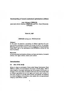
Figure 3: (a) The solid colored curves show the number of unsatis£ed clauses in the most probable con£guration x mp of each of the 4 mixtures vs iterations. The solid black line plots the expected number of violations, and the dashed black line shows the approximation to the JS distance. (b) The solid colored curves show the evolution of the G value of the best xmp con£gurations for each of 5 mixtures versus number of iterations. The dashed black line shows the corresponding approximation to the JS distance. multipliers are updated. The initial temperature is 0.1. We plot the number of constraints violated in the most probable state of each mixture as a function of the number of updates. as well as the expected number of violated constraints. After 8000 steps three distinct solutions have been found along with a fourth con£guration which violates a single constraint. 6.2

Minimization of N K Functions

The N K model de£nes a family of tunably dif£cult optimization problems [8]. The energy of N binary variables is de£ned as the average of N contributions local to each variable xi and involving 0 ≥ K ≥ N − 1 other randomly chosen variables x1i · · · xK i : PN −1 1 K K+1 G(x) = N local con£gurations E i is i=1 Ei (xi ; xi , · · · xi ). For each of the 2 assigned a value drawn uniformly from 0 to 1. K controls the number of local minima; under Hamming neighborhoods K = 0 optimization landscapes have a single global optimum and K = N − 1 landscapes have on average 2N /(N + 1) local minima. Further properties of N K landscapes may be found in [?]. Fig. 6.1(b) plots the energy of a 5 mixture model for a multi-modal N = 300 K = 2 function. The K − 1 spins other than i upon which Ei depends were selected at random. At termination of the PC algorithm 5 distinct con£gurations are obtained with the nearest pair of solutions having Hamming distance 12.

7

Conclusion

A distributed constrained optimization framework based on probability collectives has been presented. Motivation for the framework was drawn from an extension of full-rationality game theory to bounded rational agents. An algorithm that is capable of obtaining one or more solutions simultaneously was developed and demonstrated on two problems. The results show a promising, highly distributed, off-the-shelf approach to constrained optimization. There are many avenues for future exploration. Alternatives to the Lagrange multiplier

method used here can be developed for constraint satisfaction problems. By viewing the constraints as separate objectives, a Pareto-like optimization procedure may be developed whereby a gradient direction is chosen which is constrained so that no constraints are worsened. This idea is motivated by the highly successful WalkSAT [?] algorithm for k-sat in which spins are ¤ipped only if no previously satis£ed clause becomes unsatis£ed as a result of the change. Probability collectives also offer promise in devising new methods for escaping local minima. Unlike traditional optimization methods where monotonic transformations of the objective leave local minima unchanged, such transformations will alter the local minima structure of the Lagrangian. This observation, and alternative Lagrangians (see [?] for a related approach using a different minimization criterion) offer new approaches for improved optimization.

References [1] D. H. Wolpert. Factoring a canonical ensemble into a product of ensembles. 2003. preprint cond-mat/0307630. [2] D. H. Wolpert. Bounded rational games, information theory, and statistical physics. In D. Braha and Y. Bar-Yam, editors, Complex Engineering Systems, 2004. [3] D. H. Wolpert. Generalizing mean £eld theory for distributed optimization and control. 2004. submitted. [4] T. Cover and J. Thomas. Elements of Information Theory. Wiley-Interscience, New York, 1991. [5] R. O. Duda, P. E. Hart, and D. G. Stork. Pattern Classi£cation (2nd ed.). Wiley and Sons, 2000. [6] T. S. Jaakkola and M. I. Jordan. Improving the mean £eld approximation via the use of mixture distributions. In M. I. Jordan, editor, Learning in Graphical Models. Kluwer Academic, 1998. [7] M. Mezard, G. Parisi, and R. Zecchina. Analytic and algorithmic solution of random satis£ability problems. Science, June 2002. [8] S. A. Kauffman and S. A. Levin. Towards a general theory of adaptive walks on rugged landscapes. Journal of Theoretical Biology, 128:11–45, 1987.