Proceedings of the 1999 lEEE
International Conference on Robotics & Automation Detroit, Michigan May 1999
Distributed Control of Flexible Transfer System (FTS) Using Learning Automata Toshio FUKUDA*', Kosuke SEKIYAMA*~,Yoshiaki HASEBE*3, Yasuhisa HASEGAWA*~ Susumu SHIBATA*~,Hironobu YAMAMOTO*~ and Yuji INADA*4 "Center for Cooperative Research in Advanced Science and Technology, "Department of Mechano-Informatics and Systems, School of Engineering, Nagoya University, Furo-cho, Chikusa-ku, Nagoya 464-8603, JAPAN Phone: +8 1-52-789-448I, Fax: +8 1-52-789-3909 Email: { fukuda@mein,
[email protected],yasuhisa@mei n) .nagoya-u.ac.jp *2Departmentof Management and System Science, The Science University of Tokyo, Suwa College 5000- 1 Toyohira, Chino, Nagano 39 1-0292 JAPAN Phone: +8 1-266-73-1201 ex. 335
Fax: +8 1-266-73-1230 Email:
[email protected] *4Mechatronics Technology Section Advanced Industrial Systems Technology Dept. Technology Research & Development Center Toyo Engineering Corporation 8-1, Akanehama 2-chome Narashino-shi, Chiba, 275-0024 JAPAN Email: (s-shibata,yamamoto,inada-y) @is.toyoeng.co.jp Tel: +8 1-47-454-1794. Fax: +8 1-47-454-163
Abstract This paper proposes a flexible transfer system (FTS) as one of the self-organizing manufacturing systems. The FTS is composed of autonomous robotic modules, which transfer a palette carrying an object. Through the selforganization of a multi-layered strategic vector field corresponding to a task, the FTS can generate quasioptimal transfer path in fully distributed way. We apply the learning automata for path generation algorithm. Simulation is conducted to evaluate the basic performance of the system and the results show the feasibility of application. Also, the developed hardware is explained.
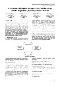
1. Introduction The large-scale production systems, such as mobile production line and heavy industrial plants are still based on the centralized control. In the centralized control systems, optimization of the productivity or efficiency is expected in a rather stationary environment, while several problems have been pointed out with regard to fault-tolerance, flexibility, and expansion of the system configurations to cope with a dynamical change of work environment. These problems will become more conspicuous for further complicated and larger systems. Therefore, a distributed autonomous system with a capability of self-organization has been required, because it is superior to the centralized system in the features of load distribution and higher adaptability[l]. In this research, we propose Flexible Transfer System (ITS) as an example of the self-organizing production system, which is shown in fig.1. The I;TS transfers a pallet on an autonomous robotic module,
Fig. 1 Flexible Transfer System where an assembling part is put. Based on the local communication between the connected modules and local information processing, a successful transferring path is generated. The configuration of modules can be changed according to a kind of task. For example, a situation can be considered where a part of module is broken down, or a configuration has to be modified for the maintenance of a module. Due to the self-organizing capability, the FTS can cope with the changes without suspending a function of the whole system. The purpose of self-organizing transferring path is attaining a .quasi-optimized state, which means that it is not optimized in the sense of the centralized control based on the global information. Where, the central issue is how to control the direction of the self-organization for a quasi-optimized state. The conventional work on the distributed control and selforganizing production system is as follows. The FTS using GA realizes suitability for scheduling transportation program[2][3]. In Flat Transportation of
Micro system research, Micro Actuator responds to system order autonomously[4][5]. Mobile Robot makes the way around using Fuzzy Rule and Learning Automata[6]. In this paper, we present a distributed control method using the learning automata for the FTS. As a first stage of the work, we simulated a process of self-organization of the particular transferring path for an assembling task, and evaluated a basic performance of the system. The algorithm can be easily implemented to the developed experimental system as shown in fig. I . 2. Flexible Transfer System (FTS) 2.1 Configuration of the FTS The FTS is composed of many autonomous transfer modules, which system configuration is depicted in fig.2. Any four sides of the module can be connected with another transfer module and the connected modules are communicable through Ethernet. Each module recognizes an existence of the palette with equipped proximity switches, and it transfers a palette to the neighboring module driven by the Omni-wheels. The direction of transfer is restricted in the x-y direction, in order to guarantee that a module can correctly recognize the palette on it. Figure 3 illustrates the surface of the robotic module and the bottom of palette. The palette carries an object to be assembled. A data carrier chip is installed in the center of the bottom side of palette where the machining information of the object is written down. When the module recognizes a palette on it with proximity switches, it will read the task information of the object from the data carrier, and decides the direction to transfer the palette. Pallet
(I
Proximity Switch
II
I F 1)
YD ReadlWrite AC Motor Amplifier Unit
2.2 Basic Approach for the FTS Control Each module has no global information such as a configuration of the whole modules, or the location of itself. What the module can obtain is the peripheral condition of itself through the communication. However, the FTS will generate a feasible path from random state, in the fully distributed way. The central idea of FTS is a self-organization of multi-layered strategic vector fields. Each module has an action strategy, which is defined as a vector value. Local interactions among the modules develop the global stochastic vector field, which corresponds to a particular machining task. Once a strategy filed is generated, the palette can reach to the desired machining site by referring the vector field wherever it may be placed. The concept is depicted in fig.5. For generation of the strategy field, we apply the learning automata, as described in the following section.
Robot
Palette
: Data Carrier Chip
: Metal Chip
0 : I D ReadJWrite Amplifier Unit : Proximity Switch 0: Omni Wheel Fig.3 Module and Palette
It
Palette Patern
Strategic Vector Field
Total 25 units
Fig.:! System Configuration of FTS
Fig.4 Strategic Vector Field 3. Distributed Control of FTS by Learning Automata 3.1 Learning Automata In this section, we describe a brief introduction of the learning automata[7][8]. The learning automata are defined by a set of six variables of the real number, which indicates a set of input to the automaton as shown in fig.5. That is given as,
( x,n,A, ~ ( t F) , G)
(1)
Hence, i2 = {a,, a, ;.-,a,} is a state set of the automaton, and ~ = @ , , a ~ , . . . , a ~ } ( s 2isr )a set of the output from the automaton. Also, n (t) = (n, (t), n ,(t), ,n,(t))is defined as a state probability vector at time t(= 1,2,.-.), based on which a particular state of the automaton w(t) is determined stochastically. That is, w(t) = w, is selected by the 0 . .
probability n,(t). F is an algorithm to update a state vector. If a response to the automaton is given by .r(t) for an action a(t) ,n (t) is updated based on the followings n(t + 1) = ~ ( n ( t )a(t), , XU)) (2) G is the output function which gives a correspondence between the state and the action, but here, it isssets of r dimensional vectors, given by
(3)
g, = (gJ,,g,29...,g,,)(j =1,2,...,s)
Then, an action a; is determined based on the stochastic vector g j for respective statew, . For this automaton, environment is characterized by unknown probabilistic distribution 8 (i = 1,2,-.-,r ) on X , corresponding to a;(i = 1,2,...,r ) .
strategy vector field to determine where to transfer the palette. Env(x, y) and h(x, y, s, t) correspond to i2 and n (t) in the section 3.1. Now, we define the set of neighborhood of the module as follows, p(i)={(x+1,y)(x,y-1)(x-l,~),(x,~+1)}
(4)
where, i indicates an element of the set. The strategy vector of the module located at p stochastically determines the direction of transfer of the palette, which is now expressed as follows, hp(s3t)=
(b0(l)1bp(2)9bp(3)9
bp(4))T
(5)
3.2.2 Learning Algorithm of Strategy Vector When a module successfully transfers the palette to the machining site of corresponding task, it will receive a constant reward from the machining site. However, since the FTS is fully distributed system, modules, which are not connected to the machining site, cannot explicitly know what is a correct behavior. Therefore, we introduce a reward variable rp(s,t) for each module corresponding to the kind of task s ex.^, B, C) . When a module m[a] transfers a palette to the module m[b], m[a] will receive a reward from m[b], which value is a constant ratio of r,, (s, t)of m[b]. This procedure is expressed by[9],
stationary raldom
x(t)= xj E X
environment (8 ,p,,...,el learning a(t)=aiE A
automaton
4
rp(s9t + I)= (1 - k)rp (s,t>+ k rp(rrr8n.~) (k = const)
(6)
Through this procedure, a field of the reward is organized, where a module closer to the machining site will have a larger reward value. This implies that a gradient of the reward field is generated. Hence, we define a vector, which element is a relative value between the neighboring modules of positionp. This is given by,
(x,Q,A,z(~)F,G) Fig.5 Learning Automata
3.2 Self-organizing Algorithm of Strategic Vector Field 3.2.1 Strategic Vector Field We apply the learning automaton to the path organization of the FTS. Let be p = (x, y) a position of the module, and Ethe set of the position. Also, the peripheral condition of the module (existence of another palette) is defined by Env(x, y), which can be recognized by the communication between the modules. The internal state of the module is represented as h(x, y, s, t ) , where s and t indicates the kind of task, and time step respectively. The set of h(x, y,s,t) gives a
Using (), the reward vector is defined as follows, a Rp (s, t)= (I - a ) r + n [0,1I Ctl rp(i)GJ) Where, the second term is four-dimensional vector of normalized random numbers. This is introduced to restrict initial fluctuations due to the excessive dependence to the reward values in the initial stage of the learning process. The reward vector is essential because it gives the direction of self-organization of the strategy vectors. Now, the strategy vector (5) is updated based on the following rule, hP(s,r+1)= ~ ( (+l~,(s,t)).h~(s,t)) 1 (9)
Where, 1is unit matrix of order 4, which is simply introduced to correct the dimension of vector. Also, F is an operator to normalize norm of the vector.
3.2.3 Collision Avoidance Since the FTS transfers multiple palettes in a fully distributed way, there is a case where the designated module of transference is occupied by the other palette. Therefore, the occupation of the module should be confirmed before the transference, by way of the communication between the modules. According to the negotiation, the strategy vector has to be modified if needed, to avoid a collision. The occupation is checked as follows, 1 Pi : empty spti)(t) = {O , :occupied
basically not required, but it is assumed for just simplification and for the future plan of fusion with another algorithm, which is undergoing work. Each module functions as a learning automaton, and selforganizes a strategic vector field for a feasible transfer path according to the placement of the machining sites. Each module will get the task information of the object
(Exit)
Based on (1O), sp(t)= (s,(,)(tlsp(2,(tl~,,3)(tlsp(4,~t))T Env, (t)=
1sP(t)
(11) (12)
By use of (12), the strategy vector is modified such that the module will not transfer the palette to the occupied module, which is given by h;(s,r + I)= p(EnvP(t). hp (s,t +I)) (13)
C (J
(Exit)
Fig.6 Example of Flexible Transfer System
The actual palette transference is performed based on (13). 4. Simulation Experiments We exemplify the I T S with the proposed algorithm and evaluate the basic performance of the system. Figure 6 illustrates the supposed task environment in the simulation. From the entrance, a palette is thrown into the system. As is mentioned in section 2, the information of the object is contained as to what kind of task should be executed in the data carrier of the palette. The marked A, B, and C in fig.6 indicates the machining site for such a particular task. In this example, the object on the palette is needed three kinds of task. If a machining schedule is designated as A + B + C in the data carrier, the palette has to be transferred through a feasible path. When the task is completed, the palette will exit from the machining site (Exit). 4.1 Generation of Strategic Vector Field We observe how the strategic vector will evolve in the model. For this simulation, following assumptions are set, (1) 5 X 5 modules (2) 4 directions for the transfer (3) Synchronized transfer (4) 3 machining sites (5) 1 time step for a palette transfer Hence, the synchronized transfer (3) as a whole system is
v Fig. 7 Path Image on the palette. According to the task information, corresponding strategic field is referred. At the initial condition, the strategic vector field is randomized. So, the motion of the palette exhibits a random walk. However, as the learning process proceed, the vector field converges to an effective state. Figure 6 shows an example of the generated path of the palette, which corresponds to fig.6. From the left side of entrance, a palette is transferred into the system, where three kinds of machining tasks are planned but its order is not strictly defined. The palette will exit from a machining site in case where all of the tasks are finished. In this example, a possible efficient path is A B C , or A + C + B . Since the configuration of vector field is dependent on the initial condition and a process of evolution, which may be affected by a local congestion of palettes, the
generated vector field could be not optimal but feasible to provide successful path. Figure 8 shows an actual simulation screen, where the left side is a situation of the palette placement and the right side is a well developed strategic vector filed corresponding to the left side state. Three different kinds of vector field are depicted.
the FTS continuously generates vector field, moderate congestion can be resolved. As shown in fig.9 (d), the system fails to deal with more than 4 palettes in this configuration. Since each palette has a different task, the occupation of the path by the another palette often disturbs successful organization of vector filed. We can notice that, until around 150 time steps, the FTS can modify the strategic vector very well, the vector field lose high flexibility after long time steps. This is a fundamental problem of the current stage of proposed algorithm. We are aware of how this takes place. It is due to saturation of the reward vector, not because of the learning ability of the algorithm. Now, we are working on this problem from various approaches. The average required time steps for respective cases are summarized in table 1.
Fig. 8 Simulation Image
I
4.2 Estimation of the Basic Performance We evaluate the basic performance of the FTS. Apparently, there will be a limitation in the number of palettes the FTS can deal with at the same time. For typical two cases, simulations are performed. In both cases, the task is set to visit two machining sites of three. 4.2.1 The case where the number of palette is constant Firstly, let us consider the case where the number of palette is constant in the FTS. This corresponds to the situation that only the object is thrown to and sent out from the system, but palettes just go around on the modules carrying the object. Now, assume that there are k palettes on the transfer modules. Simulations were performed for the following cases, Case A1 : Case A2: CaseA3: Case A4:
k k k k
=l
=2 =3 =4
(fig.9 (a)) (fig.9 (b)) (fig.9 (c)) (fig.9 (d))
Figure 9 shows the results for the respective cases. In fig.9, the horizontal axis indicates the trial numbt~rof palette, which transferred the object, and the vertical axis indicates the re-quired time step for the completion of tasks. For all cases, the initial condition of the strategic vector field is random state. In case 1, because there is always only one palette on the modules, the optimal vector field is generated without difficulties. In case 2, although it takes longer time step for convergence of the strategic vector field, very efficient transfer is realized after convergence of the vector field likewise case 1. In case 3, since three palettes exit on the modules, sometimes congestion takes place, which may hinder smooth transfer in the narrow working space. Because
I
Table 1 Average task completion time (1) CaseAl CaseA2 I CaseA3 1 CaseA4 8.81Step I 11.99Step I 22.19 Step Y
I
0
1
I
0 0
0
100
200
300
0
100
200
Palette
Palette
(a)
(b)
100
200
300
0
100
200
Palette
Palette
(c)
(d)
300
300
Fig.9 Task completion time for each palette (I)
4.2.2 The case where the palette is thrown in the constant rate In the next, we examine the case where the palette is thrown at the constant rate to the FTS. Now, let us consider the case where a palette is thrown once per k steps in the system, as follows, Case B 1: Case B2: Case B3: Case B4:
k k k k
=5 =6 =7 =8
(Fig. (Fig. (Fig. (Fig.
10(a)) 1 O(b)) 10(c)) 10(d))
Figure 10 shows the results for the respective cases. Likewise fig.9, the horizontal and vertical axis is the trial number of palette, and the task completion time for the
palette respectively. Also, the initial state of the strategic vector is randomized. In caseB 1, as shown in fig. lO(a), the transfer cannot catch up with the speed of input rate. For the palette to visit two machining sites, at least 8 steps are required (see fig.8), and the self-organization requires many steps at the first stage. Therefore, the system will fall into a deadlock in the first stage before the vector filed is generated. In case B2 and B3, although the initial stage of the task execution requires long time steps, the developed vector field can cope with an amount of task efficiently. In case B4, the performance is almost optimal. Also, we can see that the overall performance is very good once after the strategic vector is self-organized. However, we see that conditions at the initial stage should be moderate until the vector field is established, although the system can manage to solve the congestion of the path. The average required time steps in the simulation are shown in table 2. According to table 2, there is a little difference in the performance where the strategic vector is successfully generated.
1
Table 2 Average task completion time (2) CaseB I CaseB2 I CaseB3 I CaseB4 1 11.81 Step 10.31 Step 11.52 Step
1
/
Palette 150 [,.
O
Palette
(a)
................................................
loo
Palette
tb)
........................................................... i
150
1
I
300
0
100 200 Palette
300
(c) Fig.10 Task completion time for each p&&te (2) 5. Summary In this paper, we proposed the flexible transfer system (FTS) composed autonomous robotic transfer modules. Despite each module can deal with only local information, the global transfer path can be generated for the task configurations. This is achieved by introducing the multi- layered strategic vector field. According to the machining information, the vector field is selected and referred for the desired path. We apply the learning automata to the self-organization of the vector field. Due to the ability of self-organization, the system possesses
high potential to cope with unknown breakdown of the transfer module and changes of the configuration, such as a location of the machining sites and extensions. Generated path is not necessarily optimal in terms of the conventional meaning of optimality, but the simulation results show the basic performance is satisfactory for the moderate conditions, which we call quasi-optimal. We confirmed that simulations of different task configurations exhibit the similar results. On the other hand, the experimental system is developed and ready for implementation. However, a fundamental problem remains to be solved, which is re-organization of the strategic vector field. We are currently working on the issue to enhance further flexibility of the ITS. This research is a part of IMS Project. References [I] T.Kohonen, "Self-Organizing MapW,Springer-Verlag ( 1995)
[2] N. Kubota, T. Fukuda and K. Shimojima, "Trajectory Planning of Cellular Manipulator System using virusevolutionary Genetic Algorithm," J. of Robotics and Autonomous System,Vol. 19, No. I , Elsevier pp.85-94 ( 1996) [3] N. Kubota, T. Fukuda, S. Shibata, H. Yamamoto and Y. Inada, "Intelligent Manufacturing System by The Evolutionary Computation -Schedule and Planning of The Flexible Transportation-," Proc. of the 23rd Intl Conf. on Industrial Electronics, Control, and Instrumentation (IECON), Vo1.3 of 4, pp1136-1141 (1997) [4] M. Ataka et al, "Fabrication and Operation of Polyimide Bimorph Actuators for Ciliary Motion System" Journal of Microelectronical Systems, vo1.2, 146-150, Dec, 1993 [5] Y. Mita et al, "Two Dimensional Micro Conveyance System with Through Holes for Electrical and Fluidic Interconnection", 9th Intl. Conf. on Solid-State Sensors and Actuators, Chicago, June, 1997 [6] T.Aoki, T.Suzuki, S.Okuma "Acquisition of Optimal Action Selection in Autonomous Mobile Robot Using Learning Automata (Experimental Evaluation)" Proc. of 1995 IEEENagoya University WWW95 on Fuzzy Logic and Neural Networks/Evolutionary Computation, pp.56-63, Nagoya, Nov, 1995 [7] K. Najim and A. S. Pozinyak, "Learning Automata Theory and Applications", PERGAMON, (1993) [8] K. S. Narendra and M. A. L. Thathachar, "Learning Automata an Introduction", Prentice-Hall, (1989) [9] Richard S. Sutton and Andrew G. Barto, "Reinforcement Learning an Introduction", The MIT Press, (1998)