The present paper develops AMC algorithms using spatially distributed sensors ... wireless sensor networks (WSNs), there has been a growing interest towards ...
DISTRIBUTED FEATURE-BASED MODULATION CLASSIFICATION USING WIRELESS SENSOR NETWORKS Pedro A. Forero, Alfonso Cano and Georgios B. Giannakis Dept. of ECE, University of Minnesota, Minneapolis, MN 55455
ABSTRACT Automatic modulation classification (AMC) is a critical prerequisite for demodulation of communication signals in tactical scenarios. Depending on the number of unknown parameters involved, the complexity of AMC can be prohibitive. Existing maximum-likelihood and feature-based approaches rely on centralized processing. The present paper develops AMC algorithms using spatially distributed sensors, each acquiring relevant features of the received signal. Individual sensors may be unable to extract all relevant features to reach a reliable classification decision. However, the cooperative in-network approach developed enables high classification rates at reduced-overhead, even when features are noisy and/or missing. Simulated tests illustrate the performance of the novel distributed AMC scheme. I. I NTRODUCTION Automatic modulation classification (AMC) of digital modulations amounts to identifying the constellation used by a digital communication system. It plays a key role in military applications ranging from eavesdropping and jamming to cognitive and software defined radios. Once a signal has been detected, the AMC algorithm chooses the modulation format from a pool of possible candidates. AMC has been widely studied and many approaches have been proposed; however, formidable challenges remain unsolved especially when the number of modulation formats is large and many unknown parameters are involved [3], [6], [1], [11], [12]. Among the notable AMC approaches, likelihood-based (LB) algorithms characterize the likelihood function of the received waveform conditioned on a particular constellation format. Selecting a modulation then reduces to testing multiple hypotheses. Viewing unknown parameters as random, leads to an optimal decision in the Bayesian sense. Work in this paper was supported by the USDoD ARO Grant No. W911NF-05-1-0283; and also through collaborative participation in the C&N Consortium sponsored by the U. S. ARL under the CTA Program, Cooperative Agreement DAAD19-01-2-0011. The U. S. Government is authorized to reproduce and distribute reprints for Government purposes notwithstanding any copyright notation thereon. 978-1-4244-2677-5/08/$25.00 2008 IEEE
However, the associated computational complexity reduces the range of applicability of these AMC schemes to cases where large processing units are available [3]. Suboptimal alternatives reduce complexity at the expense of lowering performance. Feature-based (FB) approaches on the other hand, rely on a set of features to perform the classification task [3]. Among the several FB-AMC algorithms available, those based on the methods of cumulants and moments incur manageable computational complexity relative to LB alternatives while still delivering reliable classification performance [3], [11], [12], [10]. Most existing LB and FB algorithms require data to be available at a central processing unit. With the surge of wireless sensor networks (WSNs), there has been a growing interest towards decentralized detection, estimation and classification schemes. Their advantages range from easier self-deployment to higher resilience and prolonged lifetime in hostile environments. This paper develops a cumulantbased distributed AMC algorithm using WSNs. Sensors are deployed in space and enabled to detect and process signals from their surrounding environment. By exchanging suitable information with their single-hop neighbors, individual sensors are able to classify the constellation format with accuracy as high as if they had received all other sensors’ data. Although all sensors are acquiring the same underlying signal (same transmitted symbols), the received signals at different sensors are different due to the effect of the propagation channel. This allows the novel algorithm to exploit spatial diversity which in turn boosts the classification performance. As part of the distributed AMC task, a distributed clustering algorithm along with a suitable model order selection criterion are also introduced. The distributed clustering algorithm is based on the distributed k-means algorithm in [4] and its objective is to enhance classification performance at high SNR. The rest of this paper is organized as follows. The problem of AMC using WSNs is formulated in Section 2. Section 3 deals with cumulant features for AMC, while Section 4 introduces the novel distributed AMC approach based on cumulant features. A distributed clustering approach is developed in Section 5 to determine the order of the modulation format and improve performance at high
1 of 7
SNR. Section 6 presents numerical results. II. P ROBLEM F ORMULATION The WSN is modeled as a connected set J := {1, . . . , J} of J sensors. Each sensor j can only communicate with its one-hop neighbors denoted by Nj ⊆ J . Supposing that sufficiently powerful error correcting codes are employed, inter-sensor links are considered error free. The sensors are deployed to listen (eavesdrop) a single-carrier, otherwise unknown, communication transmission of equiprobable symbols and to learn its constellation format. Individual sensors are able to estimate the carrier frequency fc , the symbol period Ts , the carrier phase θ and the frequency offset ∆f of the incoming signal. Moreover, blind equalization algorithms can be used to mitigate the effects of pulse shaping and inter-symbol interference [7, Ch. 10]. Estimates of fc can be taken from the power spectrum of the received signal and an early-late gate synchronizer can be used to estimate Ts [7, Ch. 6]. The unknown linear modulation format is indexed by m and drawn from a set M := {1, . . . , M } of M pos(m) sible modulations, where sn denotes the n-th transmitted symbol belonging to the m-th modulation format. All modulations considered are assumed zero-mean with unity average energy. The link of each sensor with the unknown transmitter is modeled as a zero-mean complex AWGN channel with variance N0 /2, where the noise is assumed uncorrelated in both time and space. After preprocessing, each sensor j stores a length-N baseband sequence rj (n) := sj (n; π j ) + wj (n), where sj (n; π j ) := A
N X
ejφj,n s(m) n z(nTs −(l−1)Ts −�j Ts ). (1)
l=1 (m)
N T The vector π j := [A, �j , g(t), {φj,n }N n=1 , {sn }n=1 , m] contains all unknown parameters after preprocessing: A is the unknown amplitude of the received signal, which is not sensor specific because the unknown transmitter is assumed to be located sufficiently far away from the WSN; �j ∈ [0, 1] is the timing offset parameter, which is different at every sensor; z(n) includes the residual channel and pulseshaping effects after matched filtering; and φj,n denotes the phase jitter. Each sensor extracts a predefined set of features from rj (n). The goal per sensor is to choose the modulation format m ∈ M that generated sj (n; π j ) based on local features along with suitable information from its single-hop neighbors with accuracy as high as if all global features were available to every sensor.
III. C ENTRALIZED F EATURE - BASED AMC Cumulant-based AMC schemes have been successfully tested to classify M-PAM, M-PSK, M-QAM and other
constellation formats [11], [12], [10]. Cumulants are of particular interest because they are relatively simple to compute and offer reasonably reliable classification performance. Furthermore, all cumulants of a Gaussian random variable of order 3 and higher are zero, a useful property for mitigating AWGN effects and detecting non-Gaussian components in a random process. Even though fourth-order cumulants will be used as classification features in this paper (second-order cumulants are also used for normalization), at the expense of increased complexity, higher-order cumulants can be included too. Next, a brief introduction to cumulants is presented. A. CUMULANTS Let x1 , x2 be two zero-mean random variables. The second-order cumulant is given by cum(x1 , x2 ) = E{x1 x2 }.
(2)
For four zero-mean random variables x1 , x2 , x3 , x4 , the fourth-order cumulant is given by cum(x1 , x2 , x3 , x4 ) = E{x1 x2 x3 x4 } − E{x1 x2 } ×E{x3 x4 } − E{x1 x3 }E{x2 x4 } − E{x1 x4 }E{x2 x3 }.
Similarly, cumulants can be defined for stationary random processes. For a zero-mean random process {x(t)}, the k -th order cumulant will be denoted as cum (x(t), x(t + τ1 ), . . . , x(t + τk )) := C k (τ1 , . . . , τk ). Notice that for zero-mean complex random variables, there are many ways to define a cumulant depending on what variables are conjugated. The p-th order q -th conjugate cumulants C pq for p = 2 are C 20 := cum(x1 , x2 ) and C 21 := cum(x1 , x∗2 ), where ∗ denotes complex conjugation. Similarly, for p = 4 cumulants will be denoted as C 40 := cum(x1 , x2 , x3 , x4 ), C 41 := cum(x1 , x2 , x3 , x∗4 ), and C 42 := cum(x1 , x2 , x∗3 , x∗4 ). For the problem at hand, rj (n) is a complex wide-sense stationary random process, and its zeroth-lag second- and fourth-order cumulants are Cj20 = E{rj2 (n)} Cj21 = E{|rj (n)|2 } Cj40 = cum(rj (n), rj (n), rj (n), rj (n)) Cj42 = cum(rj (n), rj (n), rj∗ (n), rj∗ (n)).
Note that the received signal rj (n) = sj (t; π j ) + wj (t) is the sum of two independent random variables, the random sequence of symbols and the Gaussian noise term wj (t). In the noise-free case, the unit-energy normalization is translated to C 21 = 1. In the noisy case, the noise variance is involved, leading to C 21 = 1 + E{|wj (t)|2 }. Thus, second-order cumulants must be corrected by subtracting the noise variance N0 /2, or its corresponding estimate.
2 of 7
TABLE I T HEORETICAL CUMULANTS FOR C 21 = 1 C20 1 0 0 1 1 1 1 0 0 0
Modulation BPSK QPSK 8-PSK 4-PAM 8-PAM 16-PAM 32-PAM 16-QAM 64-QAM 256-QAM
C40 -2.0000 1.0000 0.0000 -1.3600 -1.2381 -1.2094 -1.2024 -0.6800 -0.6190 -0.6047
to define a Voronoi tessellation of the feature space using a Euclidean metric. A modulation format m ∈ M is chosen ¯ − vi ||2 ≤ ||φ ¯ − vm ||2 ∀m = 1, . . . , |M| locally if ||φ j j 40 ¯ ¯ with m 6= i, and φj := [Cj , C¯j42 ]T . IV. D ISTRIBUTED F EATURE - BASED AMC
C42 -2.0000 -1.0000 -1.0000 -1.3600 -1.2381 -1.2094 -1.2024 -0.6800 -0.6190 -0.6047
Note, however, that the value of C 4q is independent of the Gaussian noise. Table I shows the cumulant values C pq for several unit variance constellations [11]. B. SAMPLE ESTIMATES OF CUMULANTS The local cumulants Cjpq are expressed in terms of the expected value of different powers of the received sequence rj (n). In practice, expectations are replaced by sample averages over the received symbols. Sample estimates of the second-order cumulants are N 1 X 2 20 ˆ Cj = rj (n) N
Cˆj21
1 = N
n=1 N X
(3) |rj (n)|2
n=1
while sample estimates of the fourth-order cumulants are N 1 X 4 40 ˆ Cj = rj (n) − 3(Cˆj20 )2 N
Cˆj42
1 = N
n=1 N X
(4) |rj (n)|4 − |Cˆj20 |2 − 2(Cˆj21 )2 .
n=1
Sample estimates of the second-order cumulants include the effect of the noise process. Hence, a local estimate of N0 /2 must be obtained and subtracted from Cˆj21 and Cˆj20 . The fourth-order cumulant estimates are compared with the cumulant values in Table I. In practice, the constellations used are not necessarily normalized to satisfy C 21 = 1; thus, for comparison purposes the fourth-order cumulant estimates must be normalized as C¯j4q = Cˆj4q /(Cˆj21 )2 . Table I shows that both C 40 and C 42 can be used to separate QAM, PAM and PSK modulations. Note also that C 42 is insensitive to phase errors caused by poor estimates of ∆f and θ. However, C 40 is scaled by ej(∆f +θ) ; and for this reason |C 40 | is used instead. A hierarchical approach to modulation classification using fourth-order cumulants can be found in [11]. Alternatively each normalized pair 40 , C 42 ]T , or, v 40 42 T vm := [Cm m := [|Cm |, Cm ] can be used m
Table I suggests that the accuracy of cumulant estimates required to distinguish between 16-PAM and 32-PAM must be better than 0.0035. In fact, the classification performance depends on how accurately the cumulants can be estimated. This motivates reducing the variance of cumulant estimates by acquiring longer sequences of symbols. The strong law of large numbers guarantees that Cˆjpq → C pq as N → ∞ with probability one. However, sensors can typically eavesdrop only a short part of the transmitted sequence. To reduce the resultant high-variance of local cumulant estimates it is thus critical for sensors to share information when computing averages in (3) and (4). A. AWGN CHANNEL MODEL Let sˆpq the sample averages involved in Cˆjpq , j denote P N 1 PN 1 4 4 ˆ41 i.e., sˆ40 j = N j = N n=1 rj (n), s n=1 |rj (n)| , and P N 1 2 with a little abuse of notation sˆ20 j = N n=1 rj (n), and 1 PN 21 2 sˆj = N n=1 |rj (n)| . For a given π j , the received symbol rj (n) is a random variable with finite variance N0 /2; hence, sˆpq j is a random variable with probability density function f (ˆ spq j ) that is not easy to characterize. However, the central limit theorem implies that for large values of N , f (ˆ spq j ) approximates a Gaussian distribution with mean pq 2 s¯ = E{ˆ spq j } and fixed variance σpq (approximate variance expressions of cumulant estimates can be found in [11]). An estimate sˆpq that combines all received symbols across sensors has variance smaller than that of a local estimate sˆpq ˆpq j . Local averages can be expressed as s j = pq pq pq s¯ + gj , j = 1, . . . , J , where gj is a complex white 2 . In zero-mean Gaussian random variable with variance σpq particular, the maximum likelihood (ML) estimator of s¯pq pq pq 1 PJ can be found in closed form as s¯ML = J j=1 sˆj . The estimator s¯pq ML is asymptotically unbiased and consistent as J → ∞. For a finite number of sensors J , is given by 2 Var(¯ spq ML ) = σpq /J . B. DISTRIBUTED FEATURE ESTIMATION Finding s¯pq ML entails computing an average of the local estimates sˆpq j . The problem of computing averages distributively using WSNs has been widely studied in recent years [13], [8], [9]. Here we adopt an approach based on the method of multipliers (MoM) because of its added resilience to noise and its fast convergence [2].
3 of 7
Let the sample average sˆpq j at sensor j be represented by pq + g pq , where the vector sˆpq = s ¯ j j T sˆpq := [