Distributed Fusion and Tracking in Multi-Sensor

Distributed Fusion and Tracking in Multi-Sensor Systems Deepak Khosla1, James Guillochon1, Howard Choe2 1

2

HRL Laboratories LLC, Malibu, CA, USA Raytheon Systems Company, NCS, Plano, TX, USA ABSTRACT

The goal of sensor fusion is to take observations of an environment from multiple sources and combine them into the best possible track picture. For simplicity, this is usually done by sending all measurements to a single node whose sole task is to fuse measurements into a coherent track picture. This paper introduces a new framework, Distributed Fusion Architecture for Classification and Tracking (DFACT), that does not rely on a single “full-awareness node” to fuse observations, but rather turns every sensor into a fusion center. Moving a network from a centralized to a distributed architecture complicates sensor fusion, but provides many tangible benefits. Since each sensor is both a source and a sink of information, the loss of any individual component means that only one of many possible information channels has been destroyed. In this paper, we discuss how to fuse both tracking and classification observations in a distributed network, and compare its performance to a centralized framework. Each track has both a kinematic state and a belief state associated with it. Components utilize the information form of the Kalman filter for kinematic tracking, while target type is determined using a hierarchical belief structure to determine object classification, recognition, and identification. Each component in the network maintains its own independent picture of the environment, and information is exchanged between components via a queued messaging system. This paper compares the performance of centralized architectures to distributed architectures, and their respective communication and computation costs. Keywords: Sensor fusion, fusion architectures, distributed fusion, distributed tracking, multi-level classification

1. INTRODUCTION Multi-sensor systems provide increased accuracy and reliability for tracking and identifying targets beyond the capabilities of isolated sensors. Other advantages include greater area coverage and robustness to failure. However, the use of multi-sensor systems have led to a tremendous increase in the amount of data requiring processing. Fusion and resource management plays a critical role in these systems. The goal of sensor fusion is to take observations of an environment from multiple sensors and combine them into the best possible track picture. Fusion architecture can be broadly classified into two distinct categories - centralized and decentralized fusion. In centralized measurement fusion, measurements from sensors are sent to a single node whose sole task is to fuse measurements into a coherent global track picture. This node is a global fusion center (Full-awareness nodes, or FAN) and it maintains the current global track state, and updates the state with incoming measurements from sensors or the passage of time. This new state can now be used to determine future states. Since centralized networks rely on a single fusion center, this makes them highly susceptible to catastrophic failure. In decentralized fusion, individual sensors combine data from other sensors to create their local track picture. In an asynchronous decentralized architecture, the measurements transmitted from each sensor are asynchronous. Each node’s state is only dependent on that node’s prior state, input from the environment, and process noise, just like any other Markovian process. Each node maintains its own individual picture of the state space, but since inter-node communication is imperfect, these state representations are often dramatically different from node to node. Moving a network from a centralized to a distributed architecture complicates sensor fusion, but provides many tangible benefits. Since each sensor is both a source and a sink of information, the loss of any individual component means that only one of many possible information channels has been destroyed. The main advantage of distributed networks is their robustness and modular nature. Our literature survey includes a number of papers that propose interesting methods for performing sensor fusion. There has been much written on the topic of centralized fusion. Thomopoulos et al.1 provide a general proof that the optimal solution to distributed fusion amounts to a Neyman-Pearson test at the fusion center and a likelihood-ratio test at the individual sensors. Architectures can use either data fusion or decision fusion, a discussion of the pros and cons of each is provided by Brooks et al.2, D’Costa and Sayeed3, and Clouqueuer et al.4 Zhang et al.5 and Wang et al.6 propose

hierarchical decision fusion: As decisions are passed up a tree of intermediate levels, certain nodes are given higher weights than other nodes depending on the quality of the fused information. We then consider the work done in distributed fusion, which is substantially less developed. Stroupe et al.7 apply distributed fusion to a network of independent robots, and explain how to properly fuse measurements received from different frames of reference. A method proposed by Xiao et al.8 involves each node updating its own data with a weighted average of its neighboring nodes. Qi et al.9 detail a system of mobile agents which travel between local data sites by transmitting themselves from one node to the next. This has the advantage of only having to transmit the agent itself, rather than the data, which could be several times larger in size. Tharmarasa et al.10 describe a distributed architecture with multiple fusion centers; however, their model still treats sensors and fusion centers as separate nodes in the network. Durrant-Whyte et al.11 present a method for tracking targets in a distributed framework; we use their information filter for the distributed architecture we present in this paper. A number of papers have explored hierarchical classification techniques. Vailaya et al12 describe a system for organizing vacation images into hierarchical categories in an effort to improve image retrieval based on image content. Koller and Sahami13 use hierarchical Bayesian classifiers to sort web pages into groups based on their respective topics. MacKay14 details the pros and cons of using Bayesian classifier models of varying complexity. In this paper we implement a new architecture to address the shortcomings of previous distributed fusion models: “Distributed Fusion Architecture for Classification and Tracking,” or DFACT. This architecture brings together several different cutting-edge technologies into a single multi-functional package, including some new technologies unique to this work. The technologies we incorporate from other sources include the information filter described in Manyika and Durrant-Whyte15 and an algorithm for debiasing polar measurements proposed by Mo et al16. We also introduce a brand new method for performing multi-level classification that is friendly to a distributed environment (see section 2.1.3). We demonstrate the combination of these technologies through a simulation test-bed written in Matlab and C++ using the MEX interface. The structure of this paper is as follows. Section 2 describes two different architecture for sensor fusion: Centralized (CFACT) and distributed (DFACT). This section details how target tracking, association, and classification are performed, and the computational and communication costs associated with each architecture. Section 3 details the simulation test bed used to test and compare the architectures presented in section 2, and includes the sensor models used and a description of the measure used to compare performance. Section 4 presents simulation results highlighting the performance differences between the architectures.. Finally Section 5 presents conclusion of this work and future directions.

2. ARCHITECTURES FOR SENSOR FUSION Sensor fusion architectures have two responsibilities - target tracking and target classification. Each track has a kinematic state (that tracks, for example, position and velocity in two dimensions) and a classification state based on a hierarchical classification scheme described in Section 2.1.3. The sensors can observe either or both of these depending on their mode of operation.

2.1 Centralized Fusion Architecture for Classification and Tracking (CFACT) In centralized tracking, the overall track picture is maintained by a single node called the “full-awareness node” (FAN). This node collects observations from all the sensors and merges the information into an updated global track picture, and then returns this updated track picture to the sensors. The centralized architecture utilizes the standard Kalman filter, we shall refer to this as the “basic” form of the Kalman filter. We make the assumption that the FAN has models of all the sensors in the network, and also knows each sensor’s current position. This means that the sensors do not have to send redundant information with each packet. A high-level diagram of the architecture’s workings is provided below.

Centralized Fusion Architecture for Classification and Tracking (CFACT) Full-Awareness Node (FAN)

Sensor 1. Make Measurements

2. Send Measurements

3. Fuse Measurements

1. Make measurements - All sensors make observations of the environment. The kinematic measurement is represented by the vector zt and the matrix Rt, while the classification measurement is represented by an ID number. 2. Send measurements - The information gathered in step 1 is sent by each sensors to the FAN. 3. Fuse measurements - First, the track pictures are updated due to the passage of time. This involves advancing the estimated state xt, the covariance matrix Pt, and the belief state bt of each of the tracks using equation . zt, Rt, and ct are then used to generate an updated state picture. This process is repeated for each sensor that returns a measurement. Figure 1. Centralized architecture for sensor fusion.

2.1.1 Tracking In this work, we assume a simplified target model. All targets have constant velocity, and are subject to random perturbation due to white noise. This allows us to use a simple Kalman filter to maintain the kinematic state. However, we use different forms of the filter for centralized and distributed fusion. It would be relatively straightforward to extend this work to other target models. The dynamics of the linear dynamical system are governed by

xt = "xt !1 + wt !1 , wt ~ N(0, Q).

(1)

Here, xt† is the state of one of the targets at time t. (If it is necessary to refer to the state of a particular target, i, a superscript will be added: xti) Φ is the state transition matrix and Q is the process noise, and N(m, Σ) denotes the multivariate normal distribution with mean vector m and covariance matrix Σ. If the target is observable at time t by sensor j (which depends on the state of the track and the action selected for the sensor), then a kinematic observation (zt,j) will be generated according to

zt , j = H t , j xt + vt , j , vt , j ~ N (0, Rt , j ).

(2)

Ht,j is the measurement transfer matrix and Rt,j is a measure of the accuracy of the measurement. We take Zt to be the set of all the kinematic observations of a track at time t. Since xt is unobservable, it must be estimated through the use of a Kalman filter17. The Kalman filter maintains a least-squares estimate x(t|t) = E[xt | Z1, …, Zt] and a covariance matrix P(t|t) = E[x(t|t)xT(t|t) | Z1, …, Zt] of the error. This is recursively maintained through the following sets of equations

xˆt (!) = "xˆt !1

(3)

Pt (!) = " t !1 Pt !1"Tt !1 + Qt !1

(4)

xˆt = xˆt (!) + K t [ zt ! H t xˆt (!)]

(5)

K t = Pt (!) H T [ H t Pt (!) H tT + R]!1

(6)

Pt = [ I ! K t H t ]Pt (!)

(7)

where xˆt is the current track estimate and Pt is the covariance associated with that estimate,

†

Like all vectors in this paper, this is a column vector.

2.1.2 Association Individual measurements are not associated with a particular track when they are generated and need to be associated with existing tracks (We do not create or delete tracks at runtime, all tracks are created based on target ground truths at t = 0). We have also included false alarms in our model, which are detection events that arise from random noise and not due to the presence of a target. These two issues make it necessary to perform track association. For this task, we have chosen to use the Hungarian method, the implementation of which is known as Munkres’ algorithm18. Assume there are M workers and N tasks, and each combination MN has an associated cost CMN. The algorithm determines which workers should perform which tasks to minimize the total cost. For our problem, the workers are the existing tracks, and the tasks are the measurements. The cost CMN is defined by the Mahalanobis distance

r r d M (x , y ) =

r

r

T

(x ! y )

r r " !1 (x ! y ) .

(8)

This is similar to the Euclidean distance; the difference being the inclusion of the covariance ! . The covariance used is that of the measurement itself. This means that if two measurements are equidistant from an existing track, but each measurement has a different ! , the measurement with the smallest covariance will be associated with the track. Association can be performed by either the sending node or the receive node, depending on the type of Kalman filter being used. The centralized architecture exhibited in this paper requires sensor nodes to forward all information to the FAN, which then performs the association. 2.1.3 Classification As with the kinematic state, the identification of the track can be reasoned about in a number of ways; we apply Bayesian reasoning to the problem. We model the sensors using confusion matrices; the klth element of Θtj gives the probability at time t that sensor j reports the track as type k when it is type l. This matrix is generated for each sensor/target combination by the FAN in CFACT, so the sensors only need to communicate a number labeling the appropriate row of the matrix to be used in the belief state update. The uncertainty is modeled as a multinomial distribution; the kth element of the belief state b(t) is the belief (i.e. probability) at time t that the track is type k, given all the observations that have come up to (and including) time t. If the track is observable at time t by sensor j, then an identification observation (otj) will be produced. We take Ot to be the set of all the identification observations of a track at time t. The belief state can then be updated with

bt =

bt !1 • otj . bt !1otj"

(9)

We now describe the process to compute the elements of the confusion matrix First, we determine the probability that an object will be identified as class k given that it is class k. The probability of correct identification P(k|k) is given by Johnson’s criteria, found in Harney19: E

(N N50 ) , E = 2.7 + .7 N P(k | k ) = E N 50 1 + (N N 50 )

(10)

N is the number of resolution elements on the target when the measurement is taken, and N50 specifies the number of resels required for a 50% chance of associating the object with the correct type. The value of N is dependent on the sensor being used; in our test bed, only electro-optical sensors are capable of performing classification. N50 depends on the perception level one is interested in. Table 1 shows the different levels of perception. We make the assumption that all incorrect identifications are equiprobable. Therefore, the probability that class k is identified as being class l, assuming that k ≠ l, is

P(k | l ! k ) = (1 " P(k | k ) ) (C " 1)

(11)

where C is the number of possible classes. In reality, a tank is more likely to be misclassified as a different type of tank rather than a type of car; the single-level classification model does not reflect this. This leads us into multi-level classification.

Table 1. Johnson’s criteria for different perception levels (from Harney19). The more resels we have on the target, the higher the perception level we are able to achieve.

1.5 resels (0.75 cycles) per critical dimension 3 resels (1.5 cycles) per critical dimension 6 resels (3 cycles) per critical dimension 12 resels (6 cycles) per critical dimension

50% detection probability 50% classification probability 50% recognition probability 50% identification probability

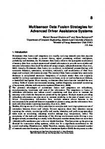
Multi-level classification enables more general information to be extracted from an object. The architectures we demonstrate in this paper incorporate a hierarchical classification structure to provide extra contextual information about each target. An example belief state is shown in Figure 2. Notice that the form of the belief state for multi-level classification remains one-dimensional. The difference arises in how the confusion matrices are constructed. Friendly

Classification

Tank

Recognition

Belief State

.1

Neutral

Humvee

.1

.02

Hostile

Car

.03

Tank

.2

.1

.2

Car

.1

.1 Van

Sedan

T90

T72

Van

Sedan

M1097

M707

Identification

.05 M109

M1

First, confusion matrices for each category and subcategory are constructed via the process detailed above, which assumes that all incorrect classifications are equiprobable. When constructing the confusion matrices, we make the assumption that each subcategory assumes that the sensor has returned a measurement that the object belong to the categories above it. Using a recursive method, we generate confusion matrices for each perception level. After we have constructed the confusion matrices, the belief state is updated using equation (9), exactly as it would under single-level classification.

Figure 2. Belief state organization.

We use the confusion matrix associated with the perception level of the observations returned from the sensor. The confusion matrix is constructed recursively, starting with the most basic object categories and progressing through more and more specific classifications through each iteration (is the object a tracked vehicle?  is the target a tank?  is the target a T72 tank?). In the simulations we run later, 3 perception levels are used (Classification, recognition, and identification). If one wants to extract categorical information from the belief state, all that is required is a simple sum of all classes that belong to that particular category. Let’s say we want to determine the chance that an object is a tank. The belief state indicates there is a 20% chance the object is a T72 tank, 10% chance it is a M1 tank, and 15% chance it is a M109 tank. Therefore, the chance that the object is a tank is simply 20% + 10% + 15% = 45%. 2.1.4 Computational Requirements The CFACT architecture uses the basic Kalman filter to maintain the track states. The basic filter is straightforward, and is suitable for architectures where there is only one fusion center. Table 2. Number of floating-point operations required to predict and update each track’s state in centralized fusion. N is the number of sensors, K is the length of the Kalman state, C is the length of the belief state, and M is the number of measured variables.

Step

Flops

Prediction

3K 3 2 K 3 + 6 MK 2 + 4 KM 2 + M 3 ! ( K 2 + 3MK ) + (3C ! 1) 3K 3 + N (2 K 3 + 6MK 2 + 4 KM 2 + M 3 + 3C ! ( K 2 + 3MK + 1))

Update Total 2.1.5 Communication Requirements

At each cycle, each sensor sends its measurements to the FAN, which requires 4(M + 1)(NFA + ND) bytes of bandwidth, where NFA is the number of false alarm events, and ND is the number of detection events.

Centralized architectures make better use of available communication resources in environments where there is little activity. Since the FAN has local models of all the sensors in the network, each measurement requires relatively little data transfer; only the measurement vector and a class identification number need to be sent for each event. For example, a measurement of a track’s position in three dimensions with three possible classifications requires a measurement size of 3 (M = 3, C = 3). Lets assume the average number of false alarm events is 0, and the number of detection events is 10. If a sensor makes a measurement every 100 ms, and there are 10 sensors, each sensor must be capable of sending 1.6 kilobytes/sec (12.8 kbps), and the FAN must be able to handle 16 kilobytes/sec (128 kbps) of incoming data transfer. Now assume that the false alarm rate is 190. Now each sensor must be capable of sending 32 kilobytes/sec (256 kbps), and the FAN must be able to handle 320 kilobytes/sec (2.56 Mbps) of incoming data transfer.

2.2 Distributed Fusion Architecture for Classification and Tracking (DFACT) The basic goal behind a distributed architecture is to make a system of sensors robust in the case of individual sensor failures. The loss of a single sensor in a decentralized environment does not substantially impact the overall health of the system. For instance, assume that our sensors are mobile platforms in a rugged environment. In such a situation, certain sensors may find themselves in areas where they cannot contact some of the other sensors. If the sensor that falls out of contact is solely responsible for maintaining the track picture, the sensor network is in trouble. The loss of an important node in a centralized network can drop system efficiency from 100% to 0%. In a decentralized system, the loss of any node might only reduce the system efficiency only marginally. In addition, the distributed architecture has lighter communication requirements in environments with dense clutter. This is because each sensor performs track association prior to sending measurements to the other sensors. Since the association algorithm will remove any measurements that are not associated with any currently existing tracks, these false alarms never have to be sent to the other sensors on the network. The amount of communications required is only dependent on the number of tracks, and will not increase with increasing clutter. Unlike CFACT, DFACT assumes that no sensor has any prior information about any other sensor. This allows sensors to be added to the network at any time, and even allows for new types of sensors to join an already existing network. However, this requires some more information to be sent between the sensors every time they communicate. This additional overhead is described in section 2.2.5. Distributed Fusion Architecture for Classification and Tracking (DFACT) 1. Make Measurements – A sensor makes an observation of the environment. 2. Generate Information – Measurements are converted to Cartesian coordinates, and the measurements are associated to pre-existing tracks. The measurements are then used to generate the information vectors I and i. 3. Share Information – The information vectors generated in step 2 and the classification measurement are transmitted to all other sensors. 4. Fuse Information – All sensors, including the sensor that made the measurement, update their own track pictures.

Figure 3. Distributed architecture for sensor fusion.

2.2.1 Tracking Our distributed model uses the Information form of the Kalman filter, derived in Grocholsky et al20. This form is mathematically identical to the basic Kalman filter, but the equations have been manipulated to reduce the complexity of updating the kinematic state with a new measurement. The steps of the Information filter are shown below.

i j ,t = H tT R !j ,1t z j ,t , I j ,t = H tT R !j ,1t H t

(12)

yt (!) = Yt (!)" t !1Yt (!) yt !1

(13)

Yt (!) = [" t !1Yt !!11"Tt !1 + Qt !1 ]!1

(14)

N

yt = yt (!) + " i j ,t

(15)

j =1

N

Yt = Yt (!) + " I j ,t

(16)

j =1

The advantage of this form of the Kalman filter lies in the ij, t and Ij, t vectors, known as the information vectors. If a platform has multiple sensors and receives multiple measurements from the same track, this platform can fuse the measurements into one set of information vectors before passing it to other nodes on the network. A caveat of this technique is that measurements must be associated with tracks before being sent. The reason for this is that the information vectors themselves contain no point of reference; they represent the adjustment required for the current state based on the new measurements. A simple 1D example: Our current estimate for a track’s position is at x = 5. A sensor produces a measurement, associates the measurement with this particular track, and then generates the information vector. The information vector specifies that the current state must be adjusted by -1.2. Thus, after the update, the new estimate is at x = 3.8. Without knowing which track we are modifying beforehand, it is impossible to associate an information vector with any given track. 2.2.2 Association Track association is performed after the measurements have been transmitted to the full-awareness node in the centralized architecture. DFACT does the inverse: The measurements are associated by each sensor to a track prior to being sent. Since the information vectors used by the distributed architecture must be attached to a specific track, association has to be done prior to communication. This saves bandwidth since measurements that are not associated with any of the tracks do not need to be sent. The method of association is identical to the centralized model, see section 2.1.2. 2.2.3 Classification DFACT uses the same multi-level classification process detailed in section 2.1.3; however, there is difference in how the measurement is communicated between the nodes. Since the centralized architecture has local models of all the sensors in the network, it only needs to receive the id number associated with the class measurement returned by each sensor. Nodes in DFACT are ignorant of the other sensors in the network, so more data is required to properly update the belief state. The nodes must send the appropriate row from the confusion matrix associated with a target at the measurement’s position. This row will have dimension 1xC, where C is the number of classes in the belief state. 2.2.4 Computational Requirements Since DFACT uses the information form of the Kalman filter, the reception of a message from another sensor node uses the computationally simple IKF update equations (15). Table 3. Floating-point operations required by the information-form of the Kalman filter used in DFACT.

Step

Flops

Information Generation

M 3 + 2MK 2 + 4 KM 2 ! ( K 2 + K ) 10 K 3 ! (2 K 2 ! K ) 2 K + (3C ! 1)

Prediction Update Total

10 K 3 + M 3 + 2 K 2 M + 4 KM 2 + KM + N (2 K + 3C ! 1) ! (3K 2 + 2 K )

This requires far fewer floating-point operations than the update procedure used in the basic Kalman filter. For a small number of sensors, this difference is negligible, but as N becomes large, the effect is substantial. 2.2.5 Communication Requirements Each sensor must send a total of 8(N – 1)(K2 + K + C + 1)ND bytes per cycle. In distributed architectures, each node sends data to every other node, and also receives information from every other node. This multiplies the number of packets required by a factor of 2(N – 1). Since each node is independent and does not have a model of the other sensors in the network, more information must be sent in each communication cycle. For a distributed architecture using the basic Kalman filter, sensors would need to include their current position, the measurement transfer matrix H, and the measurement covariance R with every transmission. DFACT does not need to include any of these matrices in its transmissions! This information is instead compactly represented by the vectors i and I. An advantage DFACT has over CFACT is that track association is done prior to message passing. This means that DFACT will not send measurements that will eventually be thrown away by the track association algorithm. Consequently, a lot less data is sent per communication cycle, especially in noisy environments. To compare, let us calculate the bandwidth required to run the example presented in the centralized section under DFACT instead: For K = 6, C = 3, N = 10, DFACT requires 33.1 kilobytes/sec (265 kbps) per sensor node. In the case where there are no false alarm events, the centralized architecture requires only a tiny fraction of the bandwidth required by DFACT. As the false alarm rate increases, the gap between the two architectures shrinks, and eventually DFACT requires less bandwidth than CFACT. Another advantage is that multiple kinematic observations of a single track can be combined prior to being sent to another node on the network. This is because both the i and I vectors can be summed prior to be sent to other nodes. This means one can reduce the communication frequency and therefore overall communication requirements. Since target kinematic states are dynamic, kinematic measurements become less accurate over time. A solution to this problem can be found in Bar-Shalom et al21. Classification observations can also be combined. For each observation, all that is sent is a single row of the confusion matrix. If we look at the form of equation (9), we notice that we can combine individual otj vectors into a single vector and perform just a single update. This means that each node can simply maintain a vector of new classification information, and send this vector at any desired frequency. However, we do not combine measurements in our simulation test-bed since we assume that each observation is sent individually.

3. SIMULATION TEST-BED Our simulation test-bed implements both the centralized and distributed architectures for the purpose of comparison. The test-bed’s Graphical User Interface (GUI) is written in Matlab, while the underlying functionality is written in C++. The two languages interact via the MEX interface, which facilitates the passage of information. We chose this setup because our goal was to create a powerful environment that is also easy to configure and assists debugging and data collection. The simulation test-bed allows us to generate various sensor and target scenarios including environmental conditions, run fusion architectures, and analyze the results. The test-bed allows us to create a scenario with variable number of targets with different starting locations and velocities. The targets are modeled as moving in the xy plane (z=0) in a straight line with constant velocity and white process noise. Since targets move in the xy plane, each target only has a four-dimensional kinematic state (comprising the position and velocity of the target along two dimensions in space). The targets is also assigned a Swerling type (I-V), and a list of classifiers that identify target class, recognition, and identification. The list of classifiers is simply a list of categories that the object belongs to. For instance, a hostile T-72 tank would be initialized with “Hostile” as its class, “Tank” as its recognition, and “T-72” as its identification. The test-bed also allows us to model variable number of radar and electro-optical (EO) sensors with different locations and parameters (see 3.2.1 and 3.2.2). While moving sensor models are allowed, the simulations presented here assumed fixed sensor positions. Both sensors return measurements in 2D polar coordinates, and these measurements are converted to a Cartesian system via the method described in Mo et al16. The test-bed also allows us to model 3D polygonal-shaped occlusions such as buildings. This effects both the sensor measurement zones and the message passing between sensors/FANs since we assume that all occlusions are completely opaque. This means that objects can only be measured/communicated with if they are within Line of Sight (LOS). The

generated terrain is fairly simple, and consists of projections of 2D polygons into the 3rd dimension. In addition, communications are subject to simple exponentially decaying packet loss functions In order to compare performance of centralized and distributed fusion architectures, we have developed several quantitative metrics. In addition to the obvious kinematic and classification errors w.r.t. ground truth, we also use information theory measures such as entropy for measures of overall performance. These measures allow us to compare joint tracking and classification performance across the architectures. They can also be used to judge how much information is gained when transitioning from one state to another. We also keep track of computation and communication resource utilization.

4. EXPERIMENTAL RESULTS We used the above simulation test-bed to generate various scenarios and compared tracking and classification performances of CFACT and DFACT approaches. We expect that the two architectures presented above should yield similar tracking/classification performance when tested side-by-side in identical environments. The results demonstrate this similarity in performance between CFACT and DFACT.

4.1 Tracking Performance First, we wish to compare the kinematic tracking performance of both architectures. To do this, we set up a scenario with a square Area Of Interest (AOI) of 2km x 2km. This AOI contains 6 radar sensors, one FAN, and 50 targets. The FAN is located at the center of the AOI. The sensors are stationary and placed randomly in 3D space with random parameters (so some radar nodes will be more effective than others). The targets are confined to move in the xy plane and assigned random Swerling types (I-V). The radar sensors only measure target position, therefore M = 2. Figure 4 shows this particular configuration. We first ran the CFACT approach on this scenario. As described in Section 2.1, the sensors make measurements on each target and send these raw measurements to the FAN. The FAN performs data association and fuses these measurements to update the global track picture. The sensors then perform measurements at the next time step and the process is repeated. At each time step, we compute the entropy of each track and the total kinematic entropy across all tracks using the formulas presented in section 3.3.

2000

FAN Sensor 1 Sensor 2 Sensor 3 Sensor 4 Sensor 5 Sensor 6 Targets

1500 ) m ( 1000 y 500

0

0

500

1000 x (m)

1500

2000

Figure 4. Environment setup. The circles represent radar sensors, the crosses represent targets, and the FAN is represented by a diamond. There are 6 radar sensors, one FAN, and 50 targets.

In DFACT, we start with the same initial scenario and conditions. As described in Section 2.2, each sensor makes measurements on the targets, performs data association and generates) the information measures described in 3.3. Each ) K sensor also acts as a fusion node. It combines its information measuresK with those it receives from other sensors/nodes to / / update Jthe track picture. Under delayed and lossy communication, Jit is expected that sensor nodes will have some ( ( differences in their track pictures. y p 1800 o r 1700 t n E 1600 c i t a m e n i K

y p 1800 o r 1700 t n E 1600

Sensor 1 Sensor 2 Sensor 3 Sensor 4 Sensor 5 Sensor 6 Centralized

1500

c i t a m e n i K

1400 1300 1200 1100 1000

0

5

10

15

20

Time Elapsed (s)

Figure 5. Kinematic entropy vs. time for each node with exponential packet loss.


1500 1400 1300 1200 1100 1000

0

5

10

15

20

Time Elapsed (s)

Figure 6. Kinematic entropy vs. time for each node with no packet loss.

Since the information form of the Kalman filter is mathematically equivalent to the basic Kalman filter, one would expect two fusion centers using these two forms of the filter with otherwise identical characteristics should perform exactly the same. The only differences we expect between the two algorithms should be due to the lossy communication and positioning of the individual nodes in the network. The results in Figure 5 show that the FAN performs better than some sensors, and worse than others. This result is expected: Since we have shown that the performance difference between the basic and information forms of the Kalman filters are negligible, all that matters is node position. In our example, the FAN is located at the center of the environment, placing it close to the center of mass of the network. The reason that certain sensors perform better than the FAN is that they are closer to the center of mass, partly due to being one of the sources of information themselves. Figure 6 shows the results of running the same test with zero packet loss. As expected, all nodes now perform identically. This is because each node now receives the same amount of information, regardless of its location. This result demonstrates the mathematical equivalence of the basic form and ) ) information forms of the Kalman filter. K / J (

4.2 Multi-Level Classification Performance

K / J (

y To test ypthe multi-level classification results, we used a similar scenario to the previous section, except now we use p o o electro-optical sensors instead of radar sensors to observe the targets. r r t n 200 E


n o i 150 t a c i 100 f i s s 50 a l C 0 0

t n 200 E

10

20 30 Time Elapsed (s)

40


n o i 150 t a c i 100 f i s s 50 a l C 0 0

50

Figure 7. Classification entropy vs. time for each node with packet loss.

10

20 30 Time Elapsed (s)

40

50

Figure 8. Classification entropy vs. time for each node with no packet loss.

This is done because the radar sensors cannot classify targets. The EO sensors make observations at the highest perception level possible, which in this case is track identification. To compare performance, we use a setup identical to the one presented in Figure 4, replacing the radar sensors with electro-optical. The results are similar to the results we obtained when comparing tracking performance. We present the case with packet loss in Figure 7 and without packet loss in Figure 8. The center of mass argument offered in the previous section serves to explain these results as well.

5. CONCLUSION This paper introduced a Distributed Fusion Architecture for Classification and Tracking (DFACT), that does not rely on a single “full-awareness node” to fuse observations, but rather turns every sensor into a fusion center. We discussed how to fuse both tracking and classification observations in a distributed framework and compare its performance to a centralized framework (CFACT). We implemented a simulation test-bed to test, validate and compare the CFACT and DFACT approaches. For the scenarios presented here, the results demonstrate that DFACT performs just as well as its centralized counterpart in terms of track and classification performance. In addition to identical performance, DFACT uses less computational resources, and in noisy environments, DFACT has milder communication requirements. We also have shown that our multi-level classification algorithm works in the context of these architectures. The current design of the test-bed is a useful tool for analysis and design of fusion architectures, but can benefit from enhancements. Future work will involve extending our test-bed to examine the influences of more realistic communication models, better tracking algorithms such as MHT as well as dynamic network topology management.

REFERENCES 1. S. Thomopoulos, R. Viswanathan, D. Bougoulias, L. Zhang, “Optimal And Suboptimal Distributed Decision Fusion,” 1988 American Control Conference, 7th, Atlanta, Ga, United States, 15-17 June 1988. Pp. 414-418. 1988 2. R.R. Brooks, P. Ramanthan, A.M. Sayeed, “Distributed Target Classification and Tracking in Sensor Networks,” Signal Processing Magazine, IEEE, vol. 19, no. 2, pp. 17-29, 2002. 3. A. D’Costa, A.M. Sayeed, “Data Versus Decision Fusion for Distributed Classification in Sensor Networks,” Military Communications Conference, 2003. MILCOM 2003. IEEE, vol. 1, pp. 585-590, 2003. 4. T. Clouqueur, P. Ramanthan, K.K. Saluja, K. Wang, “Value-Fusion versus Decision-Fusion for Fault-tolerance in Collaborative Target Detection in Sensor Networks,” Proceedings of Fourth International Conference on Information Fusion, Aug, 2001. 5. J. Zhang, E.C. Kulasekere, K. Premaratne, “Resource Management of Task Oriented Distributed Sensor Networks,” Circuits and Systems, 2001. ISCAS 2001. The 2001 IEEE International Symposium on, vol. 3, pp. 513-516, 2001. 6. X. Wang, G. Foliente, Z. Su, L. Ye, “Multilevel Decision Fusion in a Distributed Active Sensor Network for Structural Damage Detection,” Structural Health Monitoring 2006 5: 45-58 7. A.W. Stroupe, M.C. Martin, T. Balch, “Distributed sensor fusion for object position estimation by multi-robot systems,” Robotics and Automation, 2001. Proceedings 2001 ICRA. IEEE International Conference on , vol.2, no.pp. 1092- 1098 vol.2, 2001. 8. L. Xiao, S. Boyd, S. Lall, “A scheme for robust distributed sensor fusion based on average consensus,” Information Processing in Sensor Networks, 2005. IPSN 2005. Fourth International Symposium on , vol., pp. 6370, 15 April 2005 9. H. Qi, X. Wang, S.S. Iyengar, K. Chakrabarty, ”Multisensor Data Fusion in Distributed Sensor Networks Using Mobile Agents,” Proceedings of 5th International Conference on Information Fusion. Annapolis, MD, 2005 10. R. Tharmarasa, T. Kirubarajan, A. Sinha, M. L. Hernandez, “Multitarget-multisensor management for decentralized sensor networks,” Proc. SPIE Int. Soc. Opt. Eng. 6236, 62360W, 2006. 11. A. Makarenko, H.F. Durrant-Whyte, “Decentralized Data Fusion and Control in Active Sensor Networks,” 7th Int. Conf. on Info. Fusion, 2004. 12. A. Vailaya, M.A.T. Figueiredo, A.K. Jain, Z. Hong-Jiang, “Image classification for content-based indexing,” Image Processing, IEEE Transactions on , vol.10, no.1pp.117-130, Jan 2001. 13. D. Koller, M. Sahami, “Hierarchically classifying documents using very few words,” Proc. of the 14th International Conference on Machine Learning ICML97, pp. 170---178, 1997. 14. D.J.C. MacKay. “Bayesian interpolation.” Neural Computation, 4(3):415--447, May 1992. 15. J.M. Manyika, H.F. Durrant-Whyte, “An Information-theoretic Approach to Management in Decentralized Data Fusion,” Proceedings of SPIE, vol. 202, 1992. 16. L. Mo, X. Song, Y. Zhou, Z. Sun, and Y. Bar-Shalom, “Unbiased converted measurements in tracking,” IEEE Trans. Aerosp. Electron. Syst., vol. 34, July 1998, pp. 1023-1027. 17. R.E. Kalman, “A New Approach to Linear Filtering and Prediction Problems,” Transactions of the ASME— Journal of Basic Engineering, 82(D), 35–45, 1960. 18. J. Munkres, “Algorithms for the Assignment and Transportation Problems,” Journal of the Society for Industrial and Applied Mathematics, Vol. 5, No. 1, Mar., 1957, pp. 32-38 19. R. Harney, “Combat Systems vol. 1: Sensors,” 2005. 20. B. Grocholsky, H.F. Durrant-Whyte, P. Gibbens, “An Information-Theoretic Approach to Decentralized Control of Multiple Autonomous Flight Vehicles,” Proceedings of SPIE, vol. 4196, pp. 348-359, 2000. 21. Y. Bar-Shalom, C. Huimin, M. Mallick, “One-step solution for the multistep out-of-sequence-measurement problem in tracking,” Aerospace and Electronic Systems, IEEE Transactions on , vol.40, no.1pp. 27- 37, Jan 2004.