Multisensor Data Fusion: From Algorithms and ...

7

A Fuzzy Multicriteria Approach for Data Fusion André D. Mora, António J. Falcão, Luís Miranda, Rita A. Ribeiro, and José M. Fonseca

CONTENTS 7.1 Introduction........................................................................................................................... 109 7.2 Data Fusion Overview........................................................................................................... 110 7.2.1 Main Types................................................................................................................ 110 7.2.1.1 Multisensor Fusion...................................................................................... 110 7.2.1.2 Image Fusion............................................................................................... 110 7.2.1.3 Information Fusion..................................................................................... 111 7.2.2 Existing Models......................................................................................................... 111 7.2.2.1 JDL Model.................................................................................................. 111 7.2.2.2 Waterfall Model.......................................................................................... 112 7.2.2.3 Luo and Kay Model.................................................................................... 112 7.2.2.4 Thomopoulos Model................................................................................... 113 7.2.2.5 Intelligence Cycle....................................................................................... 113 7.2.2.6 Boyd Control Loop Model.......................................................................... 113 7.2.2.7 Dasarathy Model......................................................................................... 113 7.3 FIF Algorithm........................................................................................................................ 114 7.3.1 Context and Scope..................................................................................................... 114 7.3.2 FIF Architecture........................................................................................................ 115 7.4 Illustrative Applications......................................................................................................... 118 7.4.1 IPSIS—Safe Landing with Hazard Avoidance......................................................... 118 7.4.2 ILUV—UAV Landing Site Selection........................................................................ 121 7.5 Concluding Remarks............................................................................................................. 123 Acknowledgments........................................................................................................................... 123 References....................................................................................................................................... 123

7.1 INTRODUCTION This chapter discusses a recent data fusion algorithm (Ribeiro et al. 2014), Fuzzy Information Fusion (FIF), that provides a general method, based on decision matrices, for fusing heterogeneous sources, into a single composite, with the final goal of rating and ranking alternatives. In addition, FIF has the ability to handle imprecise information, either from lack of confidence in the input data or from its imprecision (allowing deviation errors). In general, FIF can be viewed as a decision support method for handling multiple criteria (i.e., input sources) classification problems under uncertain environments. We start this chapter by presenting a comprehensive overview of existing data fusion types and models, to set up the context of the discussed FIF algorithm. Then, we discuss in detail the four steps of the FIF algorithm: data normalization, uncertainty filtering, assignment of relative importance to the data sources, and data aggregation/fusion. After introducing FIF, we illustrate its potential with two applications in the aerospace domain, one for selecting the safest planet landing sites for spacecraft and another for safe landing of drones. Finally, we present some concluding remarks. 109 © 2016 by Taylor & Francis Group, LLC

110

Multisensor Data Fusion

7.2 DATA FUSION OVERVIEW Data fusion is essentially a means of combining information from multiple sources (possibly heterogeneous) into a single unified view of the various data. Khaleghi et al. (2013) and Castanedo (2013) provide an in-depth overview of past proposals and recent advances in multisource fusion. To set up the context of this work in the next two subsections we summarize the main types of data fusion and models that have been proposed for performing data fusion.

7.2.1 Main Types

Downloaded by [Andre Mora] at 14:51 26 August 2015

In general, data fusion includes three main types: multisensor, image, and information fusion. 7.2.1.1 Multisensor Fusion The main objective of multisensor fusion is to integrate data measurements extracted from different sensors and combine them into a single representation. Within this context, most approaches focus on multisensor data fusion using statistical methods (Kalman filters) and probabilistic techniques (Bayesian networks) (Waltz and Llinas 1990; Manyika and Durrant-Whyte 1994; Goodman et al. 1997; Epp et al. 2008; Lee et al. 2010). Statistical methods focus on minimizing errors between measured and predicted values, whereas probabilistic methods rely on using weighting factors based on how accurate the sensor data is. Hybrid strategies combine different multisensor fusion techniques taking the advantages of the individual approaches and mitigating their flaws. Because this type of data fusion is not applicable to this work, we will not discuss it any further. 7.2.1.2 Image Fusion The main objective of image fusion is to reduce uncertainty and redundancy while maximizing relevant information particular to an application by combining different image representations of the same scene (Goshtasby and Nikolov 2007). The general approach is to use multiple images of the same scene, provided by different sensors, and combine them to obtain a better understanding of the scene, not only in terms of position and geometry, but also in terms of semantic interpretation. Image fusion algorithms are usually divided into pixel, feature, and symbolic levels (and starting at the signal level) (Esteban et al. 2005). Feature and symbolic algorithms have not received the same level of attention as pixel-level algorithms. Pixel-level algorithms are the most common and they work either in the spatial domain or in the transformation domain. Although pixel-level fusion is a local operation, transformation domain algorithms create the fused images globally. Featurebased algorithms (symbolic) typically segment the images into regions and fuse them using their intrinsic properties (Piella 2003; Hsu et al. 2009). A summary of characteristics for this type of data fusion is depicted in Table 7.1. TABLE 7.1 Characteristics of Data Fusion Levels Characteristics

Representation Level of Information

Signal level Pixel level Feature level

Low Low Medium

Symbol level

High

Type of Sensory Information

Model of Sensory Information

Multidimensional signal Multiple images Features extracted from signals/ images Decision logic from signals/images

Random variable with noise Random process across the pixel Noninvariant form of features Symbol with degree of uncertainty

Source: Adapted from Esteban, J., A. Starr, R. Willetts, P. Hannah, and P. Bryanston-Cross. Neural Computing and Applications, 14(4):273–281, 2005.

© 2016 by Taylor & Francis Group, LLC

A Fuzzy Multicriteria Approach for Data Fusion

111


There are many suitable algorithms and techniques proposed in the literature to deal with the three levels of image fusion processes: multiresolution analysis, hierarchical image decomposition, pyramid techniques, wavelet transform, artificial neural networks, biological inspired models, fuzzy rules, principal component analysis (PCA), and so forth (Goodman et al. 1997; Piella 2003; Serrano 2006; Goshtasby and Nikolov 2007; Dong et al. 2009; Hsu et al. 2009). Good overviews on image fusion and its applications can be seen in (Piella 2003; Smith and Heather 2005; Goshtasby and Nikolov 2007). 7.2.1.3 Information Fusion As mentioned before, there is a tenuous line between image fusion and information fusion; for example, feature and symbolic levels of fusion are sometimes considered image fusion but they can also be considered as information-based fusion (Piella 2003; O’Brien and Irvine 2004). There are many interesting definitions for fusion in general, and, specifically, for information fusion as a multilevel process of integrating information from multisources to produce fused information (Lee et al. 2010). Moreover, Lee et al. (2010) discuss a list with six important factors for a successful information fusion: (1) robustness, (2) extended spatial-temporal coverage, (3) high confidence, (4) low ambiguity, (5) reliability and validity, and (6) low vulnerability. The most traditional and well-known frameworks for information fusion are based on statistical methods (e.g., Kalman filters, optimal theory, distance methods) and probabilistic techniques (e.g., Bayesian networks, evidence theory) (Waltz and Llinas 1990; Manyika and Durrant-Whyte 1994; Goodman et al. 1997; Akhoundi and Valavi 2010; Lee et al. 2010). Statistical methods focus on minimizing errors between actual and predicted values, whereas probabilistic methods rely on using weighting factors based on how accurate the data is. Interesting applications of these techniques for fusion are (Serrano 2006; Epp and Smith 2007; Rogata et al. 2007; Epp et al. 2008; Johnson et al. 2008; Shuang and Liu 2009; Li et al. 2010). Recently, computational intelligent approaches for information fusion have been proposed, particularly using Dempster–Shafer evidential theory, fuzzy set theory, and neural networks (Akhoundi and Valavi 2010; Lee et al. 2010). Some interesting applications using these novel approaches are in (Howard 2002; Serrano and Seraji 2007; Devouassoux et al. 2008; Serrano and Quivers 2008; Hsu et al. 2009; Bourdarias et al. 2010; Pais et al. 2010). In summary, information fusion models are crucial as a mean to present a coherent and uniform view to support decision makers and the respective decision-making process.

7.2.2 Existing Models Bedworth and O’Brien (2000) define a process model to be a description of a set of processes, and several models have been developed to deal with data fusion issues (Veloso et al. 2009). Considering data fusion cases, usually there is a module to deal with the sensors and their output (input module), other to make some preprocessing or full processing of the data and a module to output the data processed on the environment. The so-called adjustments/calibrations of the sensors and system itself are normally done in a closed loop interface, common in these cases (Veloso et al. 2009). 7.2.2.1 JDL Model Developed in 1985 by the United States Joint Directors of Laboratories (JDL) Data Fusion Group, the JDL data fusion model became the most common and popular conceptualization model of fusion systems (Steinberg et al. 1999). The group was intended to assist in coordinating activities in data fusion and improve communication and cooperation between development groups with the purpose of unifying research (Macii et al. 2008; Hall and Steinberg 2000; Khaleghi et al. 2013). The result of that effort was the creation of a number of activities (White 1991; Hall and Garga 1999; Steinberg et al. 1999; Hall and Steinberg 2000) such as (1) development of a process model for data fusion, (2) creation of a lexicon for data fusion, (3) development of engineering guidelines for building data fusion systems, and (4) organization and sponsorship of the Tri-Service Data Fusion Conference (e.g., from 1987 to



112


1992). The JDL Data Fusion Group has continued to support community efforts in data fusion, leading to the annual National Symposium on Sensor Data Fusion and the initiation of a Fusion Information Analysis Center. In the initial JDL data fusion lexicon (dated 1985), the group defined data fusion as “a process dealing with the association, correlation, and combination of data and information from single and multiple sources to achieve refined position and identity estimates, and complete and timely assessments of situations and threats, and their significance. The process is characterized by continuous refinements of its estimates and assessments, and the evaluation of the need for additional sources, or modification of the process itself, to achieve improved results” (Steinberg et al. 1999, p. 431). According to this model, the sources of information used for data fusion can include both local and distributed sensors (those physically linked to other platforms), or environmental data, a priori data, and human guidance or inferences (Hall and Steinberg 2000; Macii et al. 2008; Khaleghi et al. 2013). Using these sources of information, the original JDL data fusion process consists of four increasing levels of abstraction, namely, “object,” “situation,” “threat,” and “process” refinements, which were described in (Hall and Garga 1999; Steinberg et al. 1999; Hall and Steinberg 2000; Llinas and Hall 2008). To manage the entire data fusion process through control input commands of information requests, the system includes a user interface as well as a Data Management unit, a lightweight database to provide access and management of the dynamic data (Hall and Steinberg 2000; Macii et al. 2008). There are, however, some concerns with the ways in which these model levels have been used in practice. The JDL levels have frequently been interpreted “as a canonical guide for partitioning functionality within a system” (Steinberg et al. 1999); do level 1 fusion first, then levels 2, 3, and 4. The original JDL titles for these levels appear to be focused on tactical targeting applications (e.g., threat refinement), so that the extension of these concepts to other applications is not obvious (Steinberg et al. 1999). Therefore, despite its popularity, the JDL model has many shortcomings, such as being too restrictive and especially tuned to military applications, which have been the subject of several extension proposals (Hall and Llinas 1997; Steinberg et al. 1999; Llinas et al. 2004) attempting to alleviate them. In summary, the JDL formalization is focused on data (input/output) rather than processing (Khaleghi et al. 2013). 7.2.2.2 Waterfall Model As mentioned in Veloso et al. (2009), the waterfall model is a hierarchical architecture where the information output by one module will be input to the next module. This model focuses on the processing functions on the lower levels. The stages relate to the source preprocessing and levels 1, 2, and 3 of the JDL model as follows: Sensing and signal processing correspond to source preprocessing, feature extraction and pattern processing match object refinement (level 1), situation assessment is similar to situation refinement (level 2), and decision making corresponds to threat refinement (level 3) (Veloso et al. 2009). Being this similar to the JDL model, the waterfall model suffers from the same drawbacks. Although being more exact in analyzing the fusion process than other models, the major limitation is the lack of description of the feedback data flow (Bedworth and O’Brien 2000). However, Esteban et al. (2005) and Zegras et al. (2008) proposed that the sensor system is continuously updated with feedback information arriving from the decision-making module. The main aspects of the feedback element are the recalibration, reconfiguration, and data gathering alerts to the multisensor system (Esteban et al. 2005). The waterfall model does not clearly state that the sources should be parallel or serial (though processing is serial), assumes centralized control, and allows for several levels of representation (Zegras et al. 2008). This model has been widely used in the U.K. defense data fusion community but has not been significantly adopted elsewhere (Bedworth and O’Brien 2000). 7.2.2.3 Luo and Kay Model Luo and Kay (1988) presented a generic data fusion structure based in a hierarchical model, yet different from the waterfall model. In this system, data from the sensors are incrementally added on different fusion centers in a hierarchical manner, thus increasing the level of representation from the raw data or signal level to more abstract symbolic representations at the symbol level (Esteban



113

et al. 2005; Zegras et al. 2008; Veloso et al. 2009). This model has a parallel input and processing of data sources interface, which may enter the system at different stages and levels of representation. The model is based on decentralized architecture and does not assume a feedback control (Veloso et al. 2009).


7.2.2.4 Thomopoulos Model Esteban et al. (2005) and Veloso et al. (2009) mention that Thomopoulos proposed a three-level model, formed by signal level fusion, where data correlation takes place; evidence level fusion, where data are combined at different levels of inference; and dynamics level fusion, where the fusion of data is done with the aid of an existing mathematical model. Depending on the application, these levels of fusion can be implemented in a sequential manner or interchangeably (Esteban et al. 2005). At each level exists data integration preserving a given order that may cause communication problems with data transmission, and factors such as spatial (Esteban et al. 2005; Veloso et al. 2009). There will also be a database component, responsible for data gathering that will be used in a learning process (Veloso et al. 2009). 7.2.2.5 Intelligence Cycle The intelligence cycle is an approach that falls in a fusion model subgroup with cyclic character (Elmenreich 2007), with the Boyd control loop (see Section 7.2.2.6) an integral part. Intelligence processing involves both information processing and information fusion as observed in (Bedworth and O’Brien 2000). Although the information is often at a high level the processes for handling intelligence products are broadly applicable to data fusion in general (Bedworth and O’Brien 2000). The intelligence cycle model (Bedworth and O’Brien 2000; Elmenreich 2007) comprises four stages: 1. Collection: Appropriate raw intelligence data (intelligence report at a high level of abstraction) are gathered, for example, through sensors. 2. Collation: Associated intelligence reports are correlated and brought together. 3. Evaluation: The collated intelligence reports are fused and analyzed. 4. Dissemination: The fused intelligence is distributed to the users. An additional stage is enumerated by Elmenreich (2007) regarding planning and directions where the intelligence requirements are determined. However, in the particular case of the United Kingdom Intelligence Community model, this stage is subsumed in the dissemination process, unlike in the U.S. model (Bedworth and O’Brien 2000). 7.2.2.6 Boyd Control Loop Model In 1987, John Boyd proposed a cycle containing four stages that was first used for modeling the military command process (Bedworth and O’Brien 2000; Elmenreich 2007). The Boyd control loop represents the classic decision support mechanism in military information operations (Elmenreich 2007). Because decision support systems for situational awareness are tightly coupled with fusion systems, the Boyd model has also been used for sensor fusion (Bedworth and O’Brien 2000). The Boyd model has some similarities between the intelligence cycle and the JDL model. Bedworth and O’Brien (2000) and Elmenreich (2007) compared the stages of those models. Although the Boyd model represents the stages of a closed control loop system and gives an overview on the overall task of a system, the model structure is significantly limited in identifying and separating different sensor fusion tasks (Elmenreich 2007). 7.2.2.7 Dasarathy Model The Dasarathy fusion model is categorized in terms of the types of data/information that are processed and the types that result from the process (Steinberg and Bowman 2008). Its data flow is characterized


114


TABLE 7.2 The Five Levels of Fusion in the Dasarathy Model Input Data Data Features Features Decisions

Output

Analogues

Data Features Features Decisions Decisions

Data-level fusion Feature selection and feature extraction Feature-level fusion Pattern recognition and pattern processing Decision-level fusion


Source: Adapted from Bedworth, M., and J. O’Brien. IEEE Aerospace and Electronic Systems Magazine, 15:30–36, 2000.

by input/output (I/O) processes (Khaleghi et al. 2013), and three main levels of abstraction during the data fusion process are identified (Bedworth and O’Brien 2000) as: 1. Decisions: symbols or belief values 2. Features: or intermediate-level information 3. Data: or more specifically sensor data Dasarathy states that fusion may occur both within these levels and as a means of transforming between them (Bedworth and O’Brien 2000). In the Dasarathy fusion model, there are five possible categories of fusion, illustrated in Table 7.2 as types of I/O considered (Steinberg and Bowman 2008). In conclusion, several models and techniques have already been proposed in the literature for data fusion; however, most of them just apply to one type of data fusion: multisource, image fusion, or information fusion. The FIF algorithm, discussed in this chapter, is a general method that can be applied to any of those types. The main difference between FIF and the described models is that FIF uses a fuzzy multicriteria approach, which, we believe, can simplify and generalize any fusion process.

7.3 FIF ALGORITHM 7.3.1 Context and Scope There are a number of issues that make information fusion a challenging task. The development of FIF (Ribeiro et al. 2014) started with trying to answer the important question posed by Maître and Bloch (1997): “How to obtain a final value for each potential solution (e.g., pixel, hypothesis) from combining different heterogeneous measurements?” In those authors’ point of view, it can be solved in three stages, as follows:

1. Transform the measures in such a way that it is possible to combine them. 2. Combine the data as transformed by the representation according to the allowed rules for the chosen framework (e.g., Bayes rule). 3. From the resulting combination make a decision in agreement with the problem.

Information fusion is related only to the first two steps: representing, transforming, cleaning, and aggregating information. The last one is already in the realm of ranking or selecting candidate alternatives (decision) and is outside the goal of obtaining a single composite of fused information. In addition, information fusion should comply with important critical success factors (Lee et al. 2010), such as (1) robustness, (2) extended spatial-temporal coverage, (3) high confidence, (4) low


115


ambiguity, (5) reliability and validity, and (6) low vulnerability. Other authors (Khaleghi et al. 2013) also pointed out different critical factors, such as data correlation, data alignment, static versus dynamic phenomena, and so forth. However, these later challenges are mostly related to image fusion and therefore not totally applicable in the FIF context. Summarizing, the FIF algorithm incorporates the first two stages and critical factors (1) to (6). FIF is a general information fusion algorithm suitable for tackling uncertain environments, particularly when there is a lack of confidence and accuracy in the input data, as well as when the criteria are heterogeneous and require intelligent normalization (Ribeiro et al. 2014).


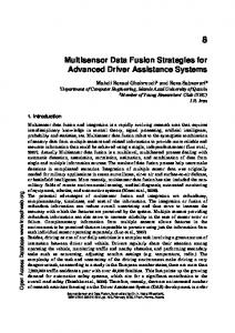
7.3.2 FIF Architecture In Figure 7.1 a complete architecture for the FIF algorithm is proposed. Each of the input data sources (i1, …, in) will run a customized data transformation process, preparing them (w1, …, wn) for the multisource data fusion. Observing Figure 7.1, it can be seen that the filtering uncertainty step is independent and should be performed before the assignment of relative importance of criteria to ensure that the data imprecision is taken into consideration when performing data fusion. Further, in FIF we strongly support that one of the best aggregation operators for fusing information is a mixture operator with weighting functions (Ribeiro et al. 2014), because it allows rewarding or penalizing poorly satisfied criteria (i.e., input variables). By extending this operator to include the uncertainty filtering the steps after normalization are jointly taken into consideration. Summarizing, the FIF algorithm includes four main steps: 1. Normalization, which includes a mathematical transformation (fuzzification) of input sources to ensure numerical and comparable data for fusion 2. Filtering uncertainty from data regarding inaccuracies and lack of confidence in input data 3. Assigning relative importance to each criteria membership value, which depends on the satisfaction/suitability of criteria for a specific alternative 4. Aggregation/fusion method (i.e., aggregation operator) for combining all fuzzified inputs (criteria) into a single composite (fused information) We next describe all the steps in detail. Step 1. Normalization Considering that inputs (criteria) can be originated by heterogeneous data sources, the inputs are normalized using fuzzy membership functions, that is, they undergo a

FIF algorithm Inputs Heterogeneous data sources

i1 i2 ...

in

Data transformation Normalization Uncertainty filtering Weighting

FIGURE 7.1 FIF algorithm architecture.


w1 w2 ...

wm

Data fusion

Output

Multisource aggregation

Fused information


116


fuzzification process (Ross 2005). Besides guaranteeing normalized and comparable data, a fuzzification method allows representing data with semantic concepts, which facilitates problem understanding. An important problem on the “variables fuzzification” is the choice of the best topology for the membership functions, because they must take into account the context objective. Hence, topologies such as triangular, trapezoidal, or Gaussian membership functions should be chosen depending on the nature of the criterion and the desirable representation and interpretation (semantic) for each criterion. Step 2. Filtering uncertainty The FIF algorithm enables dealing with the intrinsic uncertainty that can be found in the input information to be fused. The reasoning behind this step is that for any given alternative, each criterion must be adjusted by decreasing its membership value accordingly to the lack of confidence and inaccuracy (deviation interval) in the input data. This step is performed with a twofold filtering function: (1) combines metrics to deal with both types of uncertainty in the input values and (2) reflects the attitude of the decision maker (Pais et al. 2010). Lack of confidence affects all input values regarding their membership values and inaccuracy creates an interval with left and right deviations from the initial value. This function enables to adjust (decrease) the membership functions to reflect the embedded input information uncertainty and also to incorporate a pessimist or optimist view of a developer. Formally, the accuracy and confidence parameters (aij and wcj respectively) will modify the membership functions’ values using the following expression for the filtered uncertainty (Pais et al. 2010):

{

}

fuij = wc*j  1− λ* max µ( x ) − µ( xij )  *µ( xij ) (7.1) x ∈ a;b    where xij is the value of the jth criterion for site i; μ() is a membership degree in a fuzzy set; wcj is the confidence (percentage) associated to criterion j; and [a, b] is the inaccuracy deviation interval, defined as follows:

 min( D)  a=  xij − aij

 x +a ij  ij b= max( D) 

if xij − aij ≤ min( D) if xij − aij > min( D) if xij + aij ≤ max( D) D) if xij + aij > max(D

where aij is the accuracy associated to criterion j for site i, and D is the variable domain. Further, λ [0, 1] is a parameter that reflects the optimistic or pessimistic attitude of a decision maker, where close to 1 indicates a pessimistic attitude and close to 0 an optimistic attitude. Further, the accuracy value aij represents a deviation from a central value, indicating the amount of inaccuracy in the observations. It indicates that any value xij is included in the interval [xij – aij, xij + aij]. In the fusion algorithm two types of inaccuracy values are considered: absolute and relative. Absolute values, the most common, are those where the inaccuracy is independent of the input value: aij = aj. Relative values are those where the accuracy is a function of the input value xij. These will take the form of aij = aj * xij.



117

In this fashion all input values affected by any kind of uncertainty (inaccuracy or confidence) can be taken into consideration without loss of robustness. Obviously these parameters can be customized for any information fusion problem. Step 3. Weighting functions In FIF, linear weighting functions (Pereira and Ribeiro 2003; Ribeiro and Pereira 2003) are used to express the relative importance of criteria. The rationale of these weighting functions is that the satisfaction value of a criterion should influence its predefined relative importance. FIF algorithm uses a modified linear function L(x), to increase the computational efficiency and understandability, as follows (Ribeiro et al. 2014): L ( fuij ) = α


1 + βfuij , where 0 ≤ α ≤ 1 and 0 ≤ β ≤ 1 (7.2) 1+ β

where αj, βj ∈ [0, 1] and fuij is the accuracy and confidence membership value from Equation 7.1 for the jth criterion of alternative i. We can see that the parameter α is used to express the relative importance of the different criteria. The parameter β controls the ratio L(1)/L(0) = 1 + β between the maximum and minimum values of the effective generating function. When we have β = 0 (the weighting function does not depend on criteria satisfaction) it falls in the classical weighted average aggregation operator. The definition of the weighting functions morphologies is given by the parameters α and β. The α parameter provides the semantics for the weighting functions as for example (very important, important, low importance, etc.). The β parameter provides the required slope for the weighting functions to enable more or less penalization or rewarding. The α and β parameters will be set depending on the initial assigned semantic importance (e.g., important = 0.8) and on the sharpness of the function decrease, which depends on how much we want to penalize the poorly satisfied criteria. The motivation for using weighting functions in the FIF algorithm is to enable rewarding or penalizing input criteria and also to remove (filter) the imprecision in the input data regarding lack of confidence and possible inaccuracies. Step 4. Multisource aggregation The last step on FIF algorithm is to fuse the transformed input information from diverse sources. The information fusion aggregation method proposed for fusing information is based on the mixture of operators with weighting functions (Pereira and Ribeiro 2003; Ribeiro and Pereira 2003), and its general formulation is ri = ⊕ (W(fui1) ⊗ aci1,…, W(fuin) ⊗ fuin) (7.3) where • ⊕ is an aggregation method (e.g., sum, max, parametric operators) • ⊗ is a conjunction operator (e.g., multiplication, min) • fuij is the filtered uncertainty accuracy and confidence membership value of the jth input for solution i (Equation 7.1) L ( fuij ) • W ( fuij ) = n where L(fuij) is the weighting function above (Equation 7.2)

∑ L( fu ) ik

k =1

As can be observed, in FIF the weighting function of this mixture operator was extended to include dealing with imprecision. The result of this step concludes the information fusion steps of the FIF algorithm.


118


7.4 ILLUSTRATIVE APPLICATIONS The preliminary research for devising this algorithm was done in the context of past research projects, whose main goals were to recommend a safe interplanetary spacecraft target-landing site (Intelligent Planetary SIte Selection [IPSIS]) and also its adaptation for autonomously landing unmanned aerial vehicles (Intelligent Landing of Unmanned (Aerial) Vehicles [ILUV]) (more detail about these two projects is available at http://www.ca3-uninova.org). The following subsections describe how the FIF algorithm was used in these two experimental applications.


7.4.1 IPSIS—Safe Landing with Hazard Avoidance The main objective of IPSIS was to develop a model to choose the safest landing site for spacecraft with hazard avoidance and to determine when retargetings should occur. A preliminary version of the FIF algorithm was devised in IPSIS, to fuse information from shadows, textures, slopes, reachability, and fuel maps (Figure 7.2). The main publications on this project are Bourdarias et al. (2010), Pais et al. (2010), and Simoes et al. (2012). In these publications hazard maps were modeled as fuzzy functions to become the inputs for a dynamic fuzzy multicriteria model with feedback and an optimization process to answer real-time requirements. The preliminary works implied dynamic environments, several iterations, and feedback information, while here the scope is restricted to fusing information at a certain time t, without any concerns about past information. Here, we only discuss details about the fusion process and use two hazard maps (slope and texture), from the aforementioned project, to illustrate the FIF algorithm. Considering the normalization of the “low-slope,” the membership function relates to slopes lower than 20°. This criterion is normalized (“fuzzified”) with an open triangular membership function defined as follows:  1  µ( x ) =  20 − x  20 − c 

if x ≤ c if c < x ≤ 20

where x ∈ [0, 20] c = min(x) + α · (max(x) − min(x)) = 0.05* 20 = 1 α is the range of the function plateau In this case we consider α = 0.05, which results in a function plateau in the range [0, 5], although the parameter can be adjusted. The min and max values are extracted from the input matrix. Figure 7.3 depicts the input hazard map, its normalizing function, and the resulting output matrix. To illustrate the uncertainty filtering, Figure 7.4 shows its application to a membership function of “low texture.” As can be observed, we have in curve (1) the membership function representing

Camera image (shadows)

Textures (rock, craters...)

Slopes

FIGURE 7.2 IPSIS heterogeneous input data sources.


Reachability + visibility

Fuel needed

119


50 100 150 200 250 300 350 400 450 500

20

1

18 16 14 12 10 8 6 4

0.8 0.6 0.4

2

0 0

50 100 150 200 250 300 350 400 450 500

(a)

Low slope (fuzzy set)

0.2

2

4

6

8 10 12 14 16 18 20

(b)

50 100 150 200 250 300 350 400 450 500

1 0.9 0.8 0.7 0.6 0.5 0.4 0.3 0.2 0.1 0

50 100 150 200 250 300 350 400 450 500

(c)

FIGURE 7.3 Example of normalization (fuzzification) of criteria low-slope. (a) Original hazard map. (b) Membership function topology. (c) Normalized map.

0.6

0.51

102

0.4 0.31 0.2 0.0

103

101 100

0

5

10 15 20 25 30 35 Membership functions’ range: [0.00, 39.46]

10–1

0.6

2

105

103

0.51 b 0.24

0.2

106

104

0.4

0.0

(mean: 0.00, variance: 169.07) (In)accuracy: 5.00, confidence: 0.60

0.74

Membership value

104

2

2

a

0.8 Map histogram

Membership value


0.8

Criterion: texture, membership function: low texture 1 Fuzzy_Gaussian 1

1.0

0.31

102

Map histogram

Criterion: texture, membership function: low texture 106 1 Fuzzy_Gaussian (mean: 0.00, variance; 169.07) 1 2 (In)accuracy: 0.00, 105 confidence: 0.60

1.0

101 100

–5 0

5

+5

10 15 20 25 30 35 Membership functions’ range: [0.00, 39.46]

10–1

FIGURE 7.4 Example of filtering “low texture” with lack of confidence and inaccuracy.

the fuzzy set “low texture” and in curve (2) the adjusted function after using the Filter. Note that the bar charts in both graphics represent the histogram of all values in the input matrix that were used to define the membership function topology. In the left figure, we see the decrease caused in the membership function by having a confidence on the input data of only 60% but without any inaccuracy. In the right figure, we see the further decrease in the membership function by considering an inaccuracy, that is, deviation interval, of 5. In both examples we used a pessimistic attitude from the decision maker, that is, α = 1. Illustrating, to a “low-texture” value of x = 15 corresponds a membership value of μ(15) = 0.51. When we filter the information with a confidence of 60% the membership value decreases to μ(15) = 0.51 (left graphic). If we further filter the information with an (in)accuracy deviation of 5, the possible slope range is [10, 20] and the corresponding membership value decreases to μ(15) = 0.24 (right graphic). Using the same “low variance texture” example (Figure 7.4), we now exemplify in Figure 7.5 the third step of the IPSIS weighting process to express the relative importance of this criterion. The curve (3) represents the defined weighting function with parameters α = 0.8 (important criteria) and β = 0.33 (low decrease for the weight). Hence, for a texture of 15 units (x-axis) the initial membership value is 0.51. After filtering (step 2) its membership degree decreases to 0.30 and after weighting, that is, considering the relative importance of the criteria, the final value to be used for the fusion is 0.20. As can be observed, we highly penalized the input variable satisfaction value (0.51) because it displayed relatively low performance and our confidence in the data was relatively low.


120

Multisensor Data Fusion Criterion: texture, membership function: low texture


1

1 0.8

2 3 4

3 0.66

2

0.6

106

Fuzzy_Gaussian (means: 0.00, variance; 296.37)

105

(In)accuracy: 0.00, confidence: 0.60 Weight (y, alpha: 0.80, beta: 0.33)

104

y * weight

103

0.51

4

102

0.4 0.30

101

0.20

0.2

0.0

Map histogram

Membership value and resulting criteria weight

1.0

100 0

15 25 30 10 20 Membership functions’ range: [0.00, 39.46]

5

10–1

35

FIGURE 7.5 Example of hazard map importance assignment with weighting functions.

Finally, after the weighting step, the transformed inputs are fused generating the final hazard fused map (step 4 of the FIF algorithm). The multisource fusion (maps aggregation) takes place using the calculations described in the step 4 of the FIF algorithm, as described previously. From this output-fused map, the safest landing site will be the pixel with the highest ranking. The two maps to be fused (low slope and low texture), displayed in Figure 7.6, are raw input maps and the respective scale on the right shows dark for low values (objective for the fusion) and clear for good values. The fused hazard map (right) uses the same logical scale, that is, “good” alternatives are clearer and “bad” ones are in darker. The latter scale corresponds to the membership values within the interval [0, 1]. It should also be noticed that the fused hazard map (Figure 7.6, right) represents the input for the decision-making process, that is, it is the complete search space including all the potential alternatives for safe landing sites. In this fused map redder pixels correspond to best landing spots; bluer pixels represent worst landing alternatives. With this last (fusing process) we conclude the illustration of FIF algorithm in a real case study of selecting the safest landing place with hazard avoidance. Low texture

Low slope 30

50 100

25

150

20

200 250

15

300

10

350

5

400 450

50

40

100

35

150

30

200

25

250

20

300

15

350 400 450

50 100 150 200 250 300 350 400 450

45

50 100 150 200 250 300 350 400 450

Hazards fusion 50 100

0.8 0.7

150

0.6

200

0.5

250

0.4 0.3

300 350

10

400

5

450

0.2 0.1 50 100 150 200 250 300 350 400 450

FIGURE 7.6 Example of fusion of low-slope and low-variance texture hazard maps.


1 0.9

0

121



7.4.2 ILUV—UAV Landing Site Selection The ILUV was a technology transfer project to evaluate the applicability of the FIF algorithm for autonomous landing situations of a micro-UAV (Unmanned Aerial Vehicle). This project was developed within the context of the Portuguese Technology Transfer Initiative (PTTI; see http://www .ca3-uninova.org/project_iluv for more details). The main objective of ILUV was to evaluate the transfer of a space technology—IPSIS technology described previously—to “earth-based” applications. The focus was on safety landing issues of a UAV, in particular for emergency landing situations. In situations caused by motor or battery failure, FIF can be used to select a safe landing site, minimizing the risks to people and property, as well as maximizing the chances of safely recovering the aircraft. Transferring the space-oriented site selection algorithm to landing a UAV on Earth required certain adaptions. Mainly, the landing profile is different: A spacecraft will have a near vertical descent on the landing phase, while for a fixed-wing UAV the landing profile is much more horizontal. Environmental factors also come into play—in particular wind direction has a major influence on the UAV landing, whereas it is not an existing criterion on a moon landing, for example. Water features such as rivers and lakes, which pose a major hazard for a UAV, were nonexistent on the IPSIS landing on the moon and Mars. Manmade features such as roads, buildings, electrical pylons, and so forth also had to be considered. In this case the main requirements were presence of obstacles, adequate size for the landing profile, landing surface as smooth as possible, reduced slope levels, considering new criteria such as wind orientation, and safe distances from civilization—manmade structures, and so forth. Finally four criteria were selected and the respective hazard maps created: illumination, texture, shadow, and reachability. With these hazard maps the first step of FIF was applied and we defined the normalized criteria. Figure 7.7 shows a visualization of the one normalized criteria for a given iteration in the flight. Step 1 of FIF, the normalization process of constructing the memberships for the four criteria, consists of the following. Illumination (or visibility) maps specify whether a certain site (image pixel) is visible or not. Because only visible sites are desired for site selection, this criterion served Shadow map 50

50 100

100

Shadow map normalized

150

50

150 200

Shadow membership function 1 0.8

50

350

(a)

200

0.4

0

300

0

0.7

150

0.2

250

50 100

X:255 Y:1

0.6 100

150 0.8

200

150

100

250

X:165 Y:0

0

50

100

150

200

250

0.5 0.4 0.3 0.2

300 350

(b)

0.6

(c)

0.1 0

FIGURE 7.7 Example of normalization (fuzzification) of criteria shadow. (a) Original hazard map. (b) Member ship function topology. (c) Normalized map.



122


as a “mask”; only pixels with a “1” value (visible) were considered by the algorithm for suitable landing sites and therefore a crisp membership function {0, 1} was defined. Texture maps had the information related to the details of the scenario’s surface. Here the created membership function (normalization) represents “Low texture,” where near zero regions had higher ratings because they were similar to flat regions (better for landing). The Shadow map was an actual frame of the video images from the UAV flights. This set of hazard maps had a domain in the interval [0, 255]. To normalize these maps we used a simple open triangle membership function to express the transition of black (0) to white (255), within the interval [0, 1] (see Figure 7.7 for an example of one iteration). For rating purposes, brighter regions were preferred. Reachability maps provided the areas in the map where the UAV was able to reach, considering the current flight status and taking into account its flight dynamics. The normalized maps have a range within [0, 1], with 1 the desired value, which is the site with the highest probability of being reached during flight. In this case study, we skipped steps 2 and 3 of FIF because it was only a proof of concept study and the main goal was to assess the suitability of different aggregation operators for determining the safest place for landing UAVs, that is, step 4 of FIF. Three aggregation operators were used in the region aggregation process (step 4 of FIF) to find the most reliable. The two operators, Uninorm and Fimica, belong to the class of reinforcement operators (Ribeiro et al. 2010) and for comparative purposes we used the most pessimistic intersection operator, the Min operator. It should be noted that Uninorm and Fimica are full reinforcement operators, that is, they benefit “good” values in the criteria, but penalize any “bad” values, whereas the Min operator simply outputs the lowest criteria value. Validation consisted of multiple executions of the algorithm over various test scenarios. Figure 7.8 shows the outcome using the three aggregation operators. These images represent the “safety” values for each pixel if it were considered as a landing site, with values closer to 1.0 considered safer. It can be observed in Figure 7.8 that the Uninorm operator (a) is much more discriminative in terms of the aggregation process, which is in fact a good property because it favors only very good landing sites. The FIMICA operator (b) was unable to discriminate positive selecting good safety landing sites and provided too many options. The min operator also provided too many options for landing, although it was more discriminative then the FIMICA. The flexibility of the FIF algorithm allowed its easy adaptation to these criteria and specific scenario, such as the UAV landings. As a side note, the system execution also proved to be applicable to a real-world scenario, with images being retrieved from an actual flight test campaign performed by the UAV.

Uninorm

0

0.9

50

0.8

100 150 200 250 300 (a)

1

0

50

100 150 200

Fimica

0

1 0.9

50

0.8

Min

0

1 0.9

50

0.8

0.7 100 0.6 150 0.5

0.7 100 0.6 150 0.5

0.7

0.4 200 0.3 250 0.2

0.4 200 0.3 250 0.2

0.4

0.1 300 0 0

0.1 300 0 0

0.1

(b)

50

100 150 200

(c)

0.6 0.5 0.3 0.2 50

100 150 200

0

FIGURE 7.8 Safety maps for each aggregation operator; from left-to-right: (a) Uninorm, (b) Fimica, and (c) Min.



123


7.5 CONCLUDING REMARKS In this chapter, a fuzzy information fusion algorithm (FIF) was presented that uses both computational intelligence and multicriteria decision-making techniques for combining heterogeneous data sources into one fused information output. FIF fully addresses the three main challenges of any information fusion process: Data must be numerically comparable; imprecision and uncertainty must be taken into consideration; and a suitable aggregation operator must be selected to combine the information. Moreover, FIF is general enough to be applied to any problem, where the inputs may be from many different sources, as long as they can be modeled as fuzzy sets representing a semantic concept. FIF’s versatility also allows customization and tuning of the chosen parameters for expressing relative importance, as well as for the aggregation function (fusion). The FIF algorithm is divided into two main phases: the data transformation and the data fusion process. The first phase includes steps 1, 2, and 3 (normalization, filtering uncertainty, and relative criteria weighting) and transforms the heterogeneous data sources into homogeneous inputs, which then can be combined together in step 4 (fusion process). The FIF normalizes (step 1) each input data source by using fuzzy membership functions, which can be individually customized to the data. The inputs’ uncertainty (lack of confidence or imprecision) can influence a system’s behavior. In FIF an uncertainty filtering is available (step 2) for penalizing imprecise and unconfident inputs. The third step of FIF data transformation phase is the assignment of relative importance of the input criteria using penalizing/rewarding weighting functions. After the three steps of the data transformation phase, the resulting transformed inputs are finally combined using aggregation operators with weighting functions to obtain the final output ratings (e.g., a fused rated image). The algorithm’s potential was illustrated with two experimental applications in the aerospace domain, one for selecting safest planet landing sites for spacecraft and another for safe landing of drones. It should also be pointed out that FIF has the potential to be used in diverse fields including selecting suppliers, remote sensing monitoring (i.e., by combing spatial-temporal satellite images), and medical diagnoses. Some preliminary work on those topics, using parts of FIF but in a dynamic decision environment, is already published (Campanella and Ribeiro 2011; Jassbi et al. 2014). Work on other topics is already underway.

ACKNOWLEDGMENTS This work was partially supported by ESA contract (ESTEC Contract No, 21744/08/NL/CBI) and IPN contract (PTTI—National Technology Transfer Initiative in Portugal Application for a Feasibility Study-contract with UNINOVA), referring to the illustrative applications.

REFERENCES Akhoundi, M. A. A., and E. Valavi. 2010. “Multi-Sensor Fuzzy Data Fusion Using Sensors with Different Characteristics.” The CSI Journal on Computer Science and Engineering, submitted, arXiv preprint arXiv:1010.6096. Bedworth, M., and J. O’Brien. 2000. “The Omnibus Model: A New Model of Data Fusion?” IEEE Aerospace and Electronic Systems Magazine 15: 30–6. Bourdarias, C., P. Da-Cunha, R. Drai, L. F. Simões, and R. A. Ribeiro. 2010. “Optimized and Flexible MultiCriteria Decision Making for Hazard Avoidance.” In Proceedings of the 33rd Annual AAS Rocky Mountain Guidance and Control Conference. February 5–10, 2010, Breckenridge, CO: American Astronautical Society. Campanella, G., and R. A. Ribeiro. 2011. “A Framework for Dynamic Multiple-Criteria Decision Making.” Decision Support Systems 51 (1): 52–60. Castanedo, F. 2013. “A Review of Data Fusion Techniques.” The Scientific World Journal 2013: 704504. Devouassoux, Y., S. Reynaud, and G. Jonniaux. 2008. “Hazard Avoidance Developments for Planetary Exploration.” In Proceedings of the 7th International ESA Conference on Guidance, Navigation & Control Systems. June 2–5, 2008, Tralee, Ireland.



124


Dong, J., D. Zhuang, Y. Huang, and J. Fu. 2009. “Advances in Multi-Sensor Data Fusion: Algorithms and Applications.” Sensors 9: 7771–84. Elmenreich, W. 2007. “A Review on System Architectures for Sensor Fusion Applications.” Software Technologies for Embedded and Ubiquitous System, Lecture Notes in Computer Science 4761: 547–59. Epp, C. D., and T. B. Smith. 2007. “Autonomous Precision Landing and Hazard Detection and Avoidance Technology (ALHAT).” In 2007 IEEE Aerospace Conference, March 3–10, 2007, Big Sky, Montana: IEEE, pp. 1–7. Epp, C. D., E. A. Robertson, and T. Brady. 2008. “Autonomous Landing and Hazard Avoidance Technology (ALHAT).” In 2008 IEEE Aerospace Conference, March 1–8, 2008, Big Sky, Montana: IEEE, pp. 1–7. Esteban, J., A. Starr, R. Willetts, P. Hannah, and P. Bryanston-Cross. 2005. “A Review of Data Fusion Models and Architectures: Towards Engineering Guidelines.” Neural Computing and Applications 14 (4): 273–81. Goodman, I. R., R. P. Mahler, and H. T. Nguyen. 1997. Mathematics of Data Fusion. Dordrecht: Kluwer Academic Publishers. Goshtasby, A. A., and S. Nikolov. 2007. “Image Fusion: Advances in the State of the Art.” Information Fusion 8 (2): 114–8. Hall, D. L., and A. K. Garga. 1999. “Pitfalls in Data Fusion (and How to Avoid Them).” In Proceedings of the 2nd International Conference on Information Fusion—FUSION’99, July 6–8, 1999, Sunnyvale, CA, vol. 1, pp. 429–36. Hall, D. L., and J. Llinas. 1997. “An Introduction to Multisensor Data Fusion.” Proceedings of the IEEE 85 (1): 6–23. Hall, D. L., and A. N. Steinberg. 2000. “Dirty Secrets in Multisensor Data Fusion.” In National Symposium on Sensor Data Fusion, (NSSDF), June 2000, San Antonio, TX, p. 14. Howard, A. 2002. “A Novel Information Fusion Methodology for Intelligent Terrain Analysis.” In 2002 IEEE World Congress on Computational Intelligence. 2002 IEEE International Conference on Fuzzy Systems. FUZZ-IEEE’02. Proceedings (Cat. No. 02CH37291), May 12–17, 2002, Honolulu, HI: IEEE. vol. 2, pp. 1472–5. Hsu, S. L., P. W. Gau, I. L. Wu, and J. H. Jeng. 2009. “Region-Based Image Fusion with Artificial Neural Network.” World Academy of Science, Engineering and Technology 3 (5): 144–7. Jassbi, J. J., R. A. Ribeiro, and L. R. Varela. 2014. “Dynamic MCDM with Future Knowledge for Supplier Selection.” Journal of Decision Systems 23 (3): 232–48. Johnson, A. E., A. Huertas, R. A. Werner, and J. F. Montgomery. 2008. “Analysis of On-Board Hazard Detection and Avoidance for Safe Lunar Landing.” In 2008 IEEE Aerospace Conference, March 1–8, 2008, Big Sky, Montana: IEEE, pp. 1–9. Khaleghi, B., A. Khamis, F. O. Karray, and S. N. Razavi. 2013. “Multisensor Data Fusion: A Review of the State-of-the-Art.” Information Fusion 14 (1): 28–44. Lee, H., B. Lee, K. Park, and R. Elmasri. 2010. “Fusion Techniques for Reliable Information: A Survey.” International Journal of Digital Content Technology and Its Applications 4 (2): 74–88. Li, S., Y. Peng, Y. Lu, L. Zhang, and Y. Liu. 2010. “MCAV/IMU Integrated Navigation for the Powered Descent Phase of Mars EDL.” Advances in Space Research 46 (5): 557–70. Llinas, J., and D. L. Hall. 2008. “Multisensor Data Fusion.” In Handbook of Multisensor Data Fusion, edited by M. E. Liggins, D. L. Hall, and J. Llinas. Boca Raton, FL: CRC Press, pp. 1–14. Llinas, J., C. Bowman, G. Rogova, A. Steinberg, E. Waltz, W. Frank, and F. White. 2004. “Revisiting the JDL Data Fusion Model II.” In Fusion 2004: 7th International Conference on Information Fusion, edited by P. Svensson, and J. Schubert, June 28 to July 1, 2004, Stockholm, Sweden, vol. 2, pp. 1218–30. Luo, R. C., and M. G. Kay. 1988. “Multisensor Integration and Fusion: Issues and Approaches.” Proceedings of 1988 Orlando Technical Symposium. April 4, 1988, Orlando, FL, pp. 42–9. Macii, D., A. Boni, M. De Cecco, and D. Petri. 2008. “Tutorial 14: Multisensor Data Fusion.” Instrumentation Measurement Magazine, IEEE 11 (3): 24–33. Maître, H., and I. Bloch. 1997. “Image Fusion.” Vistas in Astronomy 41 (3): 329–35. Manyika, J., and H. F. Durrant-Whyte. 1994. Data Fusion and Sensor Management: A Decentralized Information-Theoretic Approach. Hemel Hempstead: Ellis Horwood. O’Brien, M. A., and J. M. Irvine. 2004. “Information Fusion for Feature Extraction and the Development of Geospatial Information.” In Fusion 2004: Seventh International Conference on Information Fusion, June 28 to July 1, 2004, Stockholm, Sweden, pp. 976–82. Pais, T. C., R. A. Ribeiro, and L. F. Simões. 2010. “Uncertainty in Dynamically Changing Input Data.” In Computational Intelligence in Complex Decision Systems, edited by D. Ruan, pp. 47–66. Paris: Atlantis Press.




125

Pereira, R. A. M., and R. A. Ribeiro. 2003. “Aggregation with Generalized Mixture Operators Using Weighting Functions.” Fuzzy Sets and Systems 137 (1): 43–58. Piella, G. 2003. “A General Framework for Multiresolution Image Fusion: From Pixels to Regions.” Information Fusion 4: 259–80. Ribeiro, R. A., and R. A. M. Pereira. 2003. “Generalized Mixture Operators Using Weighting Functions: A Comparative Study with WA and OWA.” European Journal of Operational Research 145 (2): 329–42. Ribeiro, R. A., T. C. Pais, and L. F. Simões. 2010. “Benefits of Full-Reinforcement Operators for Spacecraft Target Landing.” In Preferences and Decisions, edited by S. Greco, R. A. M. Pereira, M. Squillante, R. R. Yager, and J. Kacprzyk, 257: 353–67. Studies in Fuzziness and Soft Computing. Berlin, Heidelberg: Springer. Ribeiro, R. A., A. Falcão, A. Mora, and J. M. Fonseca. 2014. “FIF: A Fuzzy Information Fusion Algorithm Based on Multi-Criteria Decision Making.” Knowledge-Based Systems 58: 23–32. Rogata, P., E. Di Sotto, F. Câmara, A. Caramagno, J. M. Rebordão, B. Correia, P. Duarte, and S. Mancuso. 2007. “Design and Performance Assessment of Hazard Avoidance Techniques for Vision-Based Landing.” Acta Astronautica 61 (1–6): 63–77. Ross, T. J. 2005. Fuzzy Logic with Engineering Applications, 2nd Edition. New York: John Wiley & Sons. Serrano, N. 2006. “A Bayesian Framework for Landing Site Selection during Autonomous Spacecraft Descent.” In 2006 IEEE/RSJ International Conference on Intelligent Robots and Systems, October 9–15, 2006, Beijing, China: IEEE, pp. 5112–17. Serrano, N., and A. Quivers. 2008. “Evidential Terrain Safety Assessment for an Autonomous Planetary Lander.” In International Symposium on Artificial Intelligence, Robotics and Automation in Space, September 4–6, 2012, Turin, Italy. Serrano, N., and H. Seraji. 2007. “Landing Site Selection Using Fuzzy Rule-Based Reasoning.” In Proceedings 2007 IEEE International Conference on Robotics and Automation, April 10–14, 2007, Rome, Italy: IEEE, pp. 4899–904. Shuang, L., and Z. Liu. 2009. “Autonomous Navigation and Guidance Scheme for Precise and Safe Planetary Landing.” Aircraft Engineering and Aerospace Technology 81 (6): 516–21. Simoes, L. F., C. Bourdarias, and R. A. Ribeiro. 2012. “Real-Time Planetary Landing Site Selection—A NonExhaustive Approach.” Acta Futura 5: 39–52. Smith, M. I., and J. P. Heather. 2005. “A Review of Image Fusion Technology in 2005.” In SPIE 5782— Thermosense XXVII, edited by R. S. Harmon, J. T. Broach, and J. H. Holloway, Jr., Orlando, FL, March 28, 2005, vol. 5782, pp. 29–45. Steinberg, A. N., and C. L. Bowman. 2008. “Revisions to the JDL Data Fusion Model.” In Handbook of Multisensor Data Fusion, edited by M. E. Liggins, D. L. Hall, and J. Llinas, Boca Raton, FL: CRC Press, pp. 45–67. Steinberg, A. N., C. L. Bowman, and F. E. White. 1999. “Revisions to the JDL Data Fusion Model.” Proceedings of SPIE—Sensor Fusion: Architectures, Algorithms, and Applications III, April 5, 1999, Orlando, FL, vol. 3719, pp. 430–41. Veloso, M., C. Bentos, and F. Câmara Pereira. 2009. Multi-Sensor Data Fusion on Intelligent Transport Systems. MIT Portugal Transportation Systems Working Paper Series. Waltz, E. L., and J. Llinas. 1990. OLD Multisensor Data Fusion. Norwood, MA: Artech House. White, F. E. 1991. “Data Fusion Lexicon.” In The Data Fusion Subpanel of the Joint Directors of Laboratories, Technical Panel for C3, 15: 15. Zegras, C., F. Pereira, A. Amey, M. Veloso, L. Liu, C. Bento, and A. Biderman. 2008. “Data Fusion for Travel Demand Management: State of the Practice & Prospects.” In 4th International Symposium on Travel Demand Management, (TDM’08), July 16–18, 2008, Vienna, Austria.


