Distributed Genetic Process Mining Carmen Bratosin, Natalia Sidorova and Wil van der Aalst Abstract— Process mining aims at discovering process models from data logs in order to offer insight into the real use of information systems. Most of the existing process mining algorithms fail to discover complex constructs or have problems dealing with noise and infrequent behavior. The genetic process mining algorithm overcomes these issues by using genetic operators to search for the fittest solution in the space of all possible process models. The main disadvantage of genetic process mining is the required computation time. In this paper we present a coarse-grained distributed variant of the genetic miner that reduces the computation time. The degree of the improvement obtained highly depends on the parameter values and event logs characteristics. We perform an empirical evaluation to determine guidelines for setting the parameters of the distributed algorithm.
I. I NTRODUCTION Process mining has emerged as a discipline focused on the discovery of process models from data logs, i.e. recordings of previous process executions. The process models usually graphically depict the flow of work using languages as Petri Nets, BPMN, EPCs or state machines. Real life case studies performed for Phillips Medical Systems [14] or ASML [16] have shown that process mining algorithms can offer insight into processes, discover bottlenecks or errors and assist in improving processes. Most of the process mining algorithms (PMA) [2], [20] use heuristic approaches to retrieve the dependencies between activities based on patterns in the logs. However, these heuristic algorithms fail to capture complex process structures and they are not robust to noise or infrequent behavior. In [5] Alves de Medeiros proposed a Genetic Mining Algorithm (GMA) that uses genetic operators to overcome these shortcomings. The GMA evolves populations of process models towards a process model that fulfills the fitness criteria: the process model manages to replay all the behaviors observed in the log and does not allow additional ones. An empirical evaluation [6] shows that the GMA indeed achieves its goal to discover better models than other PMAs. Although the GMA prevails against other algorithms in terms of model quality, heuristic-based algorithms proved to be significantly more time efficient. We improve the time efficiency of the GMA by using a distributed environment as can be found on grid or cloud infrastructures. Genetic algorithms have a very high degree of potential parallelism [7] that can be exploited in order to improve the performance [19]. Three main distribution strategies identified in the literature [4], [7], [19] are master-slave, finegrained and coarse-grained. The first two approaches mainly Carmen Bratosin, Natalia Sidorova and Wil van der Aalst are with Department of Mathematics and Computer Science Eindhoven University of Technology P.O. Box 513, 5600 MB Eindhoven, The Netherlands email:
[email protected] [email protected] [email protected].
978-1-4244-8126-2/10/$26.00 ©2010 IEEE
speed up the algorithm by performing the fitness computation in parallel. Both methods have a high communication overhead that makes them less suitable for loosely coupled networks. The coarse-grained approach splits the population into a number of subpopulations periodically exchanging genetic material. This approach is more suitable for loosely coupled environments [18] because: (1) the method is robust to network and resource failures and (2) the communication overhead can be controlled via its parameters. In this paper, we present a Distributed Genetic Miner (DGM) that uses a coarse-grained approach suitable for the integration in a grid environment. We empirically assess the convergence of the algorithm for different inputs, i.e. we use logs with different complexities. Literature on distributed genetic algorithms [3], [8], [9], [17], [19] presents several results about the choice of the distribution parameters. However, these results are only empirically assessed for binary genetic algorithms. In our case, the individuals are graph models. We observe that some results regarding coarsegrained distributed genetic algorithms are also applicable to our algorithm. Moreover, our experimental results show that the GMA characteristics, e.g. the type of individuals, the log complexity etc., have high influence on the exact values of the parameters. The performed experiments clearly show the effect of the parameters on the DGM. Based on this we can derive general guidelines for the choice of the distribution parameters. The paper is organized as follows: Section II presents the process mining domain; Section III presents the distributed solution and its implementation. We analyze the DGM performance for different parameters combinations in Section IV. We give conclusions and describe future work in Section V. II. P ROCESS M INING In recent years, process mining has emerged as a way to analyze systems and their behavior based on event logs i.e., sequentially recorded events [2]. Unlike classical data mining, the focus of process mining is on concurrent processes and not on static or mainly sequential structures. Process mining is applicable to a wide range of systems. These systems may be pure information systems (e.g., Enterprise Resource Planning systems) or systems where hardware plays a more prominent role (e.g., embedded systems, sensor networks). The only requirement is that the system produces logs, thus recording (parts of) the actual behavior. A log describes previous executions of a process as sequences of events where each event refers to some activity. Figure 1 presents a simplified log inspired by a real-world process: handling objections against the real-estate property
(a) GMA individual
Fig. 1. A simplified log for the process of handling objections against the real-estate property valuation or tax at the Municipality of Heusden (b) The compact representation as a Causal Matrix[6]
valuation and tax at the Municipality of Heusden. This log contains information about three process instances (individual runs of a process). Each process instance is uniquely identified and has an associated trace, i.e. the executed sequence of activities. The log shows that for the process instance with id 1 the following activities, in the order of appearances, have been executed A - Register complaint, C - Analyze complaint, E - Recalculate and F - Inform complainant. For the process instances 2 and 3 two additional activities are executed: B - Suspend billing process and D - Re-initialize billing process. Each process instance starts with the execution of activity A and ends with the execution of activity F. If activity B is executed, then also activity D is executed. Based on the information shown in Figure 1, we can deduce the process model from Figure 2(a). Note that there are multiple models that can reproduce a particular log. The models quality is given by their ability to balance between underfitting and overfitting. An underfitting model allows for too much behavior while an overfitting model does not generalize enough. The computational complexity of a particular PMAs depends on the log characteristics. The following parameters give the basic characteristics of a log. • The size (S) of a log is the sum of the length of all traces. Since the complexity of PMAs is usually defined based on the size of a log, a high value of S implies long computational time and the need for a large amount of storage capacity. • The number of traces NT directly determines the significance of the obtained process models. The more traces we have, the more confident we are that the process model obtained represents the real process.
Fig. 2. GMA individual and its compact representation capturing the behavior from the example log
The number of activities NA is the number of distinguishable activities that defines the search space for the model. Simple algorithms such as the α-algorithm [2] are linear in the size of the log. However, such algorithms do not perform well on real-life data [1], [15], [16], [14] and therefore more advanced process mining algorithms are needed. For example, the α-algorithm does not capture the dependency between the activities B and D from the example log and resulting in underfitting. One of the advanced algorithms is the GMA [5], [2]. The GMA applies genetic operators on a population of process models in order to converge to models that represent precisely the input log behavior. The next section shows how GMA can be distributed. •
III. D ISTRIBUTED G ENETIC M INER In this section, we first present the advantages of using genetic algorithms in the process mining context and then we present a distributed genetic miner algorithm that uses a coarse-grained approach. In the coarse-grained approach the population is split into subpopulations. Each subpopulation runs independently and individuals are exchanged among subpopulations via migration. We can adapt this approach for any network settings by controlling the communication overhead through the choice of migration parameters. A. Genetic Process Mining The GMA [5], [6] uses genetic operators to search in the space of all possible process models for a given log. The goal
of the algorithm is to find a process model that can replay all the traces comprised in the input log. The main advantages of the GMA are the ability to discover non-trivial process structures and its robustness to noise as demonstrated by [6]. The main drawback of the algorithm is time consumption. Like for many other genetic algorithms, this is due to: 1) the time required to compute the fitness of individuals and 2) the large number of fitness evaluations needed. The GMA follows the usual steps of a classical genetic algorithm [11]. The individuals are graph models expressing activity dependencies that can be represented by a causal matrix [5]. Each node in the graph represents an activity. Each activity has an input and output condition. An example of a GMA individual is presented in Figure 2(a) and its compact representation is shown in Figure 2(b). Because A is the start activity the input condition is empty and activity A is enabled. After the execution of activity A the output condition {B OR C} is activated. Further on, the activity B is enabled because the input condition of B is only A and the output condition of A is activated. The input condition of activity C requires that either A or B are activated before activity C is enabled. If we assume that activity C is executed, we observe that B is automatically disabled because the output condition of A is not longer active. If activity B is executed, activity C remains enabled because the output condition of B {C AND D} is activated. For more details about the semantics of Causal Matrices we refer to [6], [20]. The individuals are encoded as a set of activities and their corresponding input and output conditions. Note that it is trivial to construct the graph representation from Figure 2(a) based on the compact representation from Figure 2(b). Each process model contains all the activities in the log; hence, the search space dimension depends on the number of activities in the log. The initial population is built by creating random individuals belonging to the search space. The second step of the algorithm is the fitness computation. The fitness value reflects how well an individual represents the behavior in the log with respect to completeness, that measures the ability of the individual to replay the traces from the log, and preciseness, that quantifies the degree of underfitting of log. The fitness completeness of an individual is computed by parsing the log traces. When an activity of a trace cannot be executed, i.e. the input condition is not satisfied, a penalty is given. In order to continue, the algorithm assumes that the activity was executed and it tries to parse the next activity from the trace. Additional penalties are given when the input/output conditions enable an activity incorrectly, e.g. if in the input condition, activity A and activity B are in an AND relation and in the trace only activity B is executed. In the end, the fitness quantifies all the penalties and reports them at the number of correctly parsed activities. The fitness preciseness is computed by comparing the individuals from the current population against each other. The idea is to penalize the individuals that allow more behavior than its siblings. The exact formula is out of the scope of this paper
and it can be found in [5], [6]. The execution time for the fitness computation depends on the number of traces, the average length of traces and the quality of the individual. Note that the fitness execution time increases significantly for poor quality individuals since a backward traversing of the individual is done for each non-parsed activity in order to retrieve all the incorrect input/output conditions. This property of the GMA combined with the stochastic nature of the genetic algorithm makes the overall GMA execution time difficult to predict. After the population fitness is evaluated, a new population is built by applying the genetic operators (elitism, mutation and crossover) and the newly generated population is reevaluated. The mutation modifies the input/output conditions of a randomly selected activity by insertion, removal or exchanging the AND/OR relations of the activities. The crossover exchanges the input/output conditions of a selected activity between two individuals. The algorithm generates new populations until a stop criteria is met. Possible stop criteria are: reaching a given fitness value or a predefined number of steps (generations), or no improvement for the past n generations. B. Distribution of the genetic process miner Our Distributed Genetic Miner (DGM) distributes the work using the so-called coarse-grained approach [7], [19]. Each subpopulation resides on an island and the master coordinates the islands. The role of the master is to initialize the islands by setting the initial parameters and to orchestrate the migration of individuals between the islands. In the initialization phase the master sends the log and the parameter values to each island. Note that the transfer of the log is time-consuming since our repository contains logs with file sizes varying from hundreds of kB to several gB. The islands run identical and independent GMAs, using the same parameters. The islands send information regarding their current state, such as best and average fitness, to the master. The master uses this information to coordinate the migration or to stop the DGM. The size of one individual is in the order of kBs, for example 60 kBs for the Heusden log, which implies that the communication due to the migration of individuals can cause a serious delay for DGM. We consider the following DGM parameters: 1) Selection Policy (SP) – Type of individuals sent when the migration takes place. 2) Integration Policy (IP) – How subpopulations integrate the received individuals. 3) Migration Interval (MI) – Number of generations between consecutive migrations. 4) Migration Size (MS) – Percentage of the population sent in every migration step. 5) Population Size (PS) – Number of individuals per island in each generation. 6) Number of Islands (NI) – Number of subpopulations to run in parallel.
Fig. 3.
Islands progress visualization in ProM
The first four parameters, selection policy, integration policy, migration interval and migration size define the migration policy (M P ) [4], i.e. MP = (SP , IP , MI , MS ). The SP defines the selection policy that an island uses to choose the individuals that are sent to an another island. The two most common SPs are [8] select the best individuals (SBI) and select random individuals (SRI). When an island receives new individuals, it integrates them into the current population. The most common IPs are [8] replace the worst individuals (RWI) and replace random individuals (RRI). In this paper, we propose a third method, called one step policy (OSP) which adds the new individuals to the current generation and performs one step with a larger population. We target this method especially at the settings with low population sizes, where the genetic material of relatively bad individuals can still be useful. The combination of MI and MS defines the number of individuals that an island receives. Small migration intervals lead to losing the global diversity [17] since some islands tend to dominate others. On the other hand, large migration intervals minimize the exchange between islands, slowing down the global convergence rate. We show that migration always improves performance compared to both panmictic (i.e. when the DGM runs on one island) and independent (i.e. the subpopulations do not exchange individuals) setup. The last two parameters, the population size and the number of islands, determine the degree of parallelism included in our algorithm. C. Implementation The GMA and the DGM are implemented as part of the ProM framework. The ProM framework1 is an open source Java-based plugable framework that has shown to be highly 1 See
www.processmining.org for details and for downloading the software
useful on many real-life case studies. We implemented the DGM as a collection of plug-ins: 1) The GeneticMiner plugin that implements the GMA. 2) The DistributedGeneticMinerIsland plugin implements the island algorithm. The plugin communicates with the master and other islands via a TCP/IP communication. The GeneticMiner plugin is called for the evolution steps of the subpopulation. 3) The DistributedGeneticMinerMaster plugin takes as input an log, a list of IP addresses and the values of the parameters. The master triggers via a TCP/IP communication the start of island plugins on remote ProM frameworks hosted at the given IP addresses. Each island is started with the same parameter settings. The parameters are split into two sets: GMA parameters and migration parameters. The plugin supports the definition of different migration policies and communication strategies. We implement the communication between different ProM frameworks using sockets technology. Each object (e.g. logs, individuals) is first translated to an XML based language and then sent using TCP/IP. The migration of individuals is made peer to peer between islands, the master just triggering the exchange. The sending/receiving of individuals is done asynchronously in different threads, i.e. in parallel with the main GMA. The receiving of individuals is acknowledged via shared objects between the threads. The DistributedGeneticMinerMaster plugin enables the user to monitor the progress of each island and to interact by triggering the migration or stop the evolution. Figure 3 shows a snapshot of an island progress window. The vertical lines in the graph mark the migration moments. IV. E XPERIMENTAL RESULTS In this section we evaluate the effect of the parameters values on the execution time of the DGM. The distributed genetic algorithms literature [3], [8], [9], [17], [19] presents several results about the choice of these parameters. Their results are empirically assessed for binary genetic algorithms. In our case, the individuals are graph models encoded as the sets of activities and their dependencies (the dependencies are expressed in terms of input/output condition as presented in Section III). The log characteristics have a high impact on the overall performance and influence the choice of the DGM parameters: the fitness computation for one individual depends linearly on the number of traces in the log and the required number of generations depends on the complexity of the process model and the size of the search space. However, the complexity of the process model is difficult to determine based on the log characteristics and it is an open research question. [13] proposes a number of log measurements that give some indications of the complexity of the real process. For example, the structure of a log is defined as the ratio between the size and the number of activities (i.e. S/NA ). If the structure value is far larger than the number of
TABLE I L OGS SETTINGS
Name Log A Log B Log Heusden
(a) Log A Fig. 4.
Number of activities 24 25 18
(b) Log B
Number of traces 229 300 1394
Size 3994 9054 11467
(c) Log Heusden
Execution time for “sending the best individuals” (SBI) and “sending random individuals” (SRI) policies
activities, we can conclude that the log contains repetitions and therefore complex patterns such as loops are present in the log. Obviously, the size of the search space depends on the number of activities in the log. We inspect some of the characteristics of our DGM for three different logs: A, B and Heusden. The first two logs are generated by students as part of their assignment for the process mining course. The third log is a real life log for the process of handling objections against the real-estate property valuation at the Municipality of Heusden. Table I presents the number of activities, number of traces and size for the three logs. Logs A and Heusden have a very simple structure that makes them ”easy“ from the mining point of view. Log B has a complex structure, which makes it a difficult log. The challenge of log Heusden is in the higher number of traces. In the fitness computation each individual is assessed against all the traces, which implies longer fitness computation time for Heusden. These observations can be verified in the experiments by inspecting the figures (e.g. Figure 4) for average execution time for these logs. We use a testbed of four computers with the following configurations: eight Intel(R) Xeon processors with a frequency of 2.66 GHz and 16 Gb RAM. We run each island on one processor, therefore we limit ourselves to a maximum of 32 islands. Since islands are identical from the performance point of view, we assess the results in terms of the Average Execution Time (AET) needed to find an individual with a fitness higher than 0.82 . Note that the highest possible fitness value is 1. The execution time is averaged over 40 independent runs. For the visualization and analysis of results we use SPSS3 . 2 Similar results were obtained for lower/higher stop fitness values varying from 0.6 to 0.9. 3 http://www.spss.com
The experiments show that: (1) migrating the best individuals offers better performance than migrating random ones, and (2) smaller migration intervals offer better performance. Additionally, we check the hypothesis that the OSP integration policy provides better results, especially for small population sizes than the RWP one as mentioned in Section III. A. Experimental evaluation of different migration policies As discussed in Section III, the migration policy is defined by MP = (SP , IP , MI , MS ). In this subsection we first analyze the effect of the SP and IP separately to draw conclusions about the optimal choice for the DGM. In the second part we present the influence of the combined effect of the MI and MS on the AET, using the chosen options for SP and IP. 1) Selection policy: In Figure 3 we compare the AET for two SPs: sending the best individuals (SBI) and sending random individuals (SRI) by showing the 95% confidence intervals for the AET. The experiments were performed on 32 islands each running a subpopulation of 20 individuals and migrating two individuals (MS = 10%) every 10 generations (MI =10). The differences between AETs are statistically significant according to the t-test results 4 : t(35) = 3.45, p = 0.001 for log B and t(58) = 3.153, p = 0.003 for log Heusden. For log A there is not enough statistical evidence according to the t-test results (t(78) = 1.31, p = 0.192), however the mean 4 The t-test assesses whether the means of two groups are statistically different from each other. The results are presented as: e.g. t(35) = 3.45, p = 0.001 where 35 are the degrees of freedom, t is the value of the t-distribution and p the probability that the mean difference is due by chance. A p-value smaller than 0.05 means that one time out of twenty a statistically significant difference would be found between the means even if there was none (i.e., by ”chance”).
(a) Log A: Average Execution Time
(d) Log A: Average Number of Generations
Fig. 5.
(b) Log B: Average Execution Time
(e) Log B: Average Number of Generations
(c) Log Heusden: Average Execution Time
(f) Log Heusden: Average Number of Generations
Execution time and number of generations for different combinations of migration size and migration interval
value obtained for SBI is less than the one for SRI. Based on these results we conclude that using SBI outperforms the SRI. This is consistent with the findings in [10]. For this reason, we experiment only with SBI policy in the remainder of the paper. 2) Integration policy: We compare two integration policies: replace the worst individuals policy (RWP) and one step policy (OSP). The results obtained do not show enough statistical evidence that one policy outperforms the other according to the t-test for experiments performed for different combinations of parameters values. However, on average the results for OSP are better than RWP for P S < 30 but for higher PS the RWP performs better than OSP due to the additional computation complexity. 3) Varying migration interval and migration size: Figure 4 shows the AET and the Average Number of Generations (ANG) for the three logs when we vary the migration interval and the migration size. Both AET and ANG are averaged over 40 independent runs. We also plot the results obtained when the islands are running independently without migration (M I = ∞ and M S = 0). The experiments were performed on 8 islands each running a subpopulation of 20 individuals and with migration policy SBI and OSP. We observe that for all experiments the AET when migration occurs is lower than the AET when islands run independently. The minimum AET is obtained for M I = 5
for all three logs. This contradicts the “rule of thumb” from [19] recommending to choose M I = 10 and M S = 10. The MS seems to have less importance than the MI since the values of AET for the same MI are not significantly different. The obtained results are consistent with the findings of Skolicki and De Jong in [17]. An important observation is that the reduction of AET depends on the necessary number of generations to reach the stop criteria: the reduction of AET is not significant when we use migration for logs A and Heusden because of their fast convergence (in less than 40 generations). However, the parameter settings have a high impact for log B, which only reaches the stop criteria after 400 generations. This happens because if the algorithm converges fast, the limited number of migrations that occur before convergence render the effect of migration negligible. 4) Experimental evaluation of the influence of the population size and number of islands: The total number of fitness computations is given by the number of individuals multiplied by the number of generations. The execution time is a function of the total number of fitness computations. When we use a larger PS, the number of generations is typically smaller, however much more fitness computations are performed in the first iterations when individuals have low quality implying high computation time per individual. On the other hand, using a small PS leads, in average, to
(a) Log A: Average Execution Time
(d) Log A: Average Number of Generations
Fig. 6.
(b) Log B: Average Execution Time
(e) Log B: Average Number of Generations
(c) Log Heusden: Average Execution Time
(f) Log Heusden: Average Number of Generations
Execution time and number of generations statistics for different combinations of the population size and number of islands
(a) Log A Fig. 7.
(b) Log B
(c) Log Heusden
The speed up as a ratio between the panmictic (one island) settings and the best AET on n number of islands.
a very large number of generations due to the insufficient diversity of individuals. For these reasons, the “best” AET results from a trade-off between the PS and the number of generations as confirmed in Figure 6. When N I = 1 (single island), the AET has a significantly higher value for P S = 10 than for the other values presented in the graph. A minimum is reached around P S = 60 for logs A and B and around P S = 40 for log Heusden. After the minimum value is reached, the AET increases almost linear. For N I = 2 and N I = 3 a similar tendency is observed, but the minimum is reached at a lower value. For N I > 8, the graphs shows only the linear growth since the minimum is reached for P S = 10. Note that the migration policy used for each of the experiments is: M I = 5, M S = 10%, SP = SBI, IP = OSP.
Despite the wide-spread belief [12] that large PSs are better, we observe that in our case we can use relatively small PSs to obtain the “best” AET. Figure 7 presents the speed up computed as the ratio between the minimum AET for the panmictic settings and the minimum AET on n islands. We observe that using more islands improves the obtained speed-up. However, the speed-up differs significantly for the three logs: better improvements for log B than for logs A and Heusden because of their fast convergence (in less than 40 generations). Note that the graphs suggest that there exists a threshold for the number of islands after which the speed-up stabilizes. Log Heusden has lowest threshold (at N I = 8) since its time consumption is mostly due to fitness computation. Log B has the highest threshold because of its low convergence.
Log A has a similar speed-up curve as log B, however the improvement is less significant due to its fast convergence. Moreover, we observe that even if we obtain the best speed-up using N I = 16 with P S = 10, the obtained improvement does not always justify the usage of so many islands. For example, for log A the speed-up between N I = 8 and N I = 16, i.e. the ration between the minimum AET for 8 islands and the minimum AET for 16 islands, is only 1.36. V. C ONCLUSIONS AND F UTURE W ORK Genetic process mining algorithms succeed to find better models at the price of longer computation time. In this paper, we used a coarse-grained distributed algorithm for GMA that improves its execution time. Moreover, we concluded an empirical evaluation. The potential pitfalls of DGM are time expensive data transfer and unpredictable fitness computation times. The experimental results showed that DGM significantly speeds up the computation. We empirically verified that several results for distributed genetic algorithms apply to our DGM. However, some of the typical rules of thumb do not hold for DGM. Our results confirm earlier experiences from [3], [8], [17]: (1) migrating best individuals is better than migrating random ones, (2) lower population sizes lead on average to slow convergence and higher population sizes need more fitness evaluations. Therefore the ‘‘optimal” population size has to balance between the number of generations and the population size. (3) Smaller migration intervals result in better performance. Our experiments invalidate some of widely used “rules of thumb” for distributed genetic algorithms: (1) for DGM a migration interval of 5 performs better than the traditional “rule of thumb”[19] saying that the best migration interval is equal to 10; 2) the population size per island for DGM does not need to be very large in order to have a good AET contrary to [12] that suggest to use a population size as large as possible. Moreover, our experiments suggest the existence of a threshold for the number of islands after which the obtained improvement stabilizes. The algorithm performs better for difficult process mining tasks. Although the parameters offering the best speed-ups are dependent on the log, there are some clear indications parameters settings should be chosen. Since it is very difficult to compute correlation between the parameter values and the logs characteristics, we are currently developing a self-adaptive DGM that re-adjusts the parameter values in real-time based on the DGM performance.
R EFERENCES [1] W. M. P. van der Aalst, H. Reijers, A. J. M. M. Weijters, B. F. van Dongen, A. Medeiros, M. Song, and H. M. W. Verbeek. Business Process Mining: An Industrial Application. Information Systems, 32(5):713–732, 2007. [2] W. M. P. van der Aalst, A. Weijters, and L. Maruster. Workflow Mining: Discovering Process Models from Event Logs. IEEE Transactions on Knowledge and Data Engineering, 16(9):1128–1142, 2004. [3] J. T. Alander. On optimal population size of genetic algorithms. In Proceedings of Computer Systems and Software Engineering, 6th Annual European Computer Conference, pages 65 – 70. IEEE Computer Society, 1992. [4] E. Alba and J. M. Troya. Improving flexibility and efficiency by adding parallelism to genetic algorithms. Statistics and Computing, 12(2):91–114, 2002. [5] A. K. Alves de Medeiros. Genetic Process Mining. PhD thesis, Technische Universiteit Eindhoven, Eindhoven, The Netherlands, 2006. [6] A. K. Alves de Medeiros, A. J. M. M. Weijters, and W. M. P. van der Aalst. Genetic process mining: An experimental evaluation. Data Mining and Knowledge Discovery, 14(2):245–304, 2007. [7] E. Cant´u-Paz. A survey of parallel genetic algorithms. Calculateurs Paralleles, Reseaux et Systems Repartis, 10(2):141 – 171, 1998. [8] E. Cant´u-Paz. Migration policies, selection pressure, and parallel evolutionary algorithms. Journal of Heuristics, 7(4):311–334, 2001. [9] E. Cant´u-Paz. Parameter setting in parallel genetic algorithms. In F. G. Lobo, C. F. Lima, and Z. Michalewicz, editors, Parameter Setting in Evolutionary Algorithms, volume 54 of Studies in Computational Intelligence, pages 259–276. Springer, 2007. [10] E. Cant´u-Paz and D. E. Goldberg. On the scalability of parallel genetic algorithms. Evol. Comput., 7(4):429–449, 1999. [11] D. E. Goldberg. Genetic Algorithms in Search, Optimization, and Machine Learning. Addison-Wesley Professional, January 1989. [12] D. E. Goldberg. Sizing populations for serial and parallel genetic algorithms. In Proceedings of the third international conference on Genetic algorithms, pages 70–79, San Francisco, CA, USA, 1989. Morgan Kaufmann Publishers Inc. [13] C. W. G¨unther. Process Mining in Flexible Environments. PhD thesis, Technische Universiteit Eindhoven, Eindhoven, The Netherlands, 2009. [14] C. W. Gunther, A. Rozinat, W. M. P. van der Aalst, and K. van Uden. Monitoring deployed application usage with process mining. Technical report, BPM Center Report BPM-08- 11, BPMcenter.org, 2008. [15] R. S. Mans, M. H. Schonenberg, M. Song, W. M. P. van der Aalst, and P. J. M. Bakker. Application of process mining in healthcare: A case study in a dutch hospital. Biomedical Engineering Systems and Technologies, 25:425–438, 2009. [16] A. Rozinat, I. S. M. de Jong, C. W. G¨unther, and W. van der Aalst. Process Mining Applied to the Test Process of Wafer Scanners in ASML. IEEE Transactions on Systems, Man, and Cybernetics, Part C: Applications and Reviews, 39(4):474–479, 2009. [17] Z. Skolicki and K. A. D. Jong. The influence of migration sizes and intervals on island models. In H.-G. Beyer and U.-M. O’Reilly, editors, Genetic and Evolutionary Computation Conference, GECCO 2005, Proceedings, Washington DC, USA, June 25-29, 2005, pages 1295–1302, 2005. [18] Y. Tanimura, T. Hiroyasu, and M. Miki. Discussion on searching capability of distributed genetic algorithm on the grid. Evolutionary Computation, 2003. CEC ’03. The 2003 Congress on, 2:1086–1094, Dec. 2003. [19] M. Tomassini. Spatially Structured Evolutionary Algorithms: Artificial Evolution in Space and Time (Natural Computing Series). SpringerVerlag New York, Inc., Secaucus, NJ, USA, 2005. [20] A. J. M. M. Weijters and W. M. P. van der Aalst. Rediscovering workflow models from event-based data using little thumb. Integr. Comput.-Aided Eng., 10(2):151–162, 2003.