Parallel Randomized Support Vector Machine - Semantic Scholar

Parallel Randomized Support Vector Machine Yumao Lu and Vwani Roychowdhury University of California, Los Angeles, CA 90095, USA

Abstract. A parallel support vector machine based on randomized sampling technique is proposed in this paper. We modeled a new LP-type problem so that it works for general linear-nonseparable SVM training problems unlike the previous work [2]. A unique priority based sampling mechanism is used so that we can prove an average convergence rate that is so far the fastest bounded convergence rate to the best of our knowledge. The numerical results on synthesized data and a real geometric database show that our algorithm has good scalability.

1

Introduction

Sampling theory has a long successful history in optimization [6, 1]. The application to the SVM training problem is first proposed by Balcazar et al. in 2001 [2]. However, Balcazar assumed that the SVM training problem is a separable problem or a problem that can be transformed to an equivalent separable problem by assuming an arbitrary small regularization factor γ (D and 1/k in [2] and [3]). They also stated that there were number of implementation difficulties so that no relevant results could be provided [3]. We model a LP-type problem such that the general linear nonseparable problem can be covered by our randomized support vector machine (RSVM). In order to take advantage of distributed computing facilities, we proposed a novel parallel randomized SVM (PRSVM) in which multiple working sets can be worked on simultaneously. The basic idea of the PRSVM is to randomly shuffle the training vectors among a network based on a carefully designed priority and weighting mechanism and to solve the multiple local problems simultaneously. Unlike the previous works on parallel SVM [7, 10] that lacks of a convergence bound, our algorithm, the PRSVM, on average, converges to the global optimum classifier/regressor in less than (6δ ln(N + 6r(C − 1)δ)/C iterations, where δ denotes the underlying combinatorial dimension, N denotes the total number of training vector, C denotes the number of working sites, and r denotes the size for a working set. Since the RSVM is a special case of PRSVM, our proof naturally works for the RSVM. Note that, when C = 1, our result reduces to Balcazar’s bound [3]. This paper is organized as follows. The support vector machine is introduced and formulated in the next section. Then, we present the parallel randomized support vector machine algorithm. The theoretical global convergence is given in the fourth section followed by a presentation of a successful application. We conclude our result in Section 6. W.K. Ng, M. Kitsuregawa, and J. Li (Eds.): PAKDD 2006, LNAI 3918, pp. 205–214, 2006. c Springer-Verlag Berlin Heidelberg 2006

206

2

Y. Lu and V. Roychowdhury

Support Vector Machine and Randomized Sampling

We prepare fundamentals and basic notations on SVM and randomized sampling technique in this section. 2.1

Support Vector Machine

Let us first consider a simple linear separation problem. We are seeking a hyperplane to separate of a set of positively and negatively labeled training data. The hyperplane is defined by wT xi − b = 0 with parameter w ∈ Rm and b ∈ R such that yi (wT xi − b) > 1 for i = 1, ..., N where xi ∈ Rm is a training data point and yi ∈ {+1, −1} denotes the class of the vector xi . The margin is defined by the distance of the two parallel hyperplanes wT x − b = 1 and wT x − b = −1, i.e. 2/||w||2 . The margin is related to the generalization of the classifier [12]. The support vector machine (SVM) is in fact a quadratic programming problem, which maximizes the margin over the parameters of the linear classifier. For general nonseparable problems, a set of slack variables µi , i = 1, . . . , N are introduced. The SVM problem is defined as follows: minimize (1/2)wT w + γ1T µ subject to yi (wT xi − b) ≤ 1 − µi , i = 1, ..., N µ≥0

(1)

where the scalar γ is usually empirically selected to reduce the testing error rate. To simplify notations, we define vi = (xi , −1), θ = (w, b), and a matrix X as Z = [(y1 v1 ) (y2 v2 ) ... (yN vN )]T . The dual of problem (1) is shown as follows: maximize −(1/2)αT ZZ T α + 1T α subject to 0 ≤ α ≤ γ1.

(2)

A nonlinear kernel function can be used for nonlinear separation of the training data. In that case, the gram matrix ZZ T is replaced by a kernel matrix k(x, x˜) ∈ RN ×N . Our PRSVM that is described in the following section can be kernelized and therefore is able to keep the full advantages of the SVM. 2.2

The Sampling Lemma, LP-Type Problem and KKT Condition

An abstract problem is denoted by (S, φ). Let X be the set of training vector. That is, each element of X is a row vector of the matrix X. Throughout this paper, we use CALLIGRAPHIC style letters to denote sets of the row vectors of a matrix denoted by the same letter with italian style. Here, φ is a mapping from a given subset XR of X to the local solution of problem (1) with constraints corresponding to XR and S is of size N . Define V(R) := {s ∈ S\R|φ(R ∪ {s}) = φ(R)}, E(R) := {s ∈ R|φ(R\{s}) = φ(R)}.

Parallel Randomized Support Vector Machine

207

The elements of V(R) are called violators of R and the elements of E(R) are called extremes in R. By definition, we have s violates R ⇔ s is extreme in R ∪ {s}. For a random sample R of size r, we consider the expected values vr := E|R|=r (|VR |) er := E|R|=r (|ER |) Gartner proved the following sampling lemma [9]: Lemma 1. (Sampling Lemma). For 0 ≤ r < N , er+1 vr = . N −r r+1 Proof. By definitions, we have N vr = R s∈S\R [s violates R] r = R s∈S\R [s is extreme in R ∪ {s}] = Q s∈Q [s is extreme in Q] N = er+1 , r+1 where [.] is the indicator variable for the event in brackets and the last row follows the fact that the set Q has r + 1 elements. The Lemma immediately follows. The problem (S, φ) is said to be a LP-type problem if φ is monotone and local (see Definition 3.1 in [9]). Balcazar proved that the problem (1) is a LP-type problem [2]. So is the problem (2). We use the same definitions given by [9] to define the basis and combinatorial dimension as follows. For any R ⊆ S, a basis of R is a inclusion-minimal subset B ⊆ R with φ(B) = φ(R). The combinatorial dimension of (S,φ), denoted by δ, is the size of a largest basis of S. For a LP-type problem (S,φ) with combinatorial dimension δ, the sampling lemma yields vr ≤ δ

N −r . r+1

(3)

This follows that |E(R)| ≤ δ. Then, we are able to relate the definitions of the extremes, violators and the basis to our general SVM training problem (1) or (2). For any local solution θp or αp of problem (Xp , φ), the basis is the support vector set, SV p . The violators of the local solutions will be the vectors that violate the Karush-Kuhn-Tucker (KKT) necessary and sufficient optimality conditions. The KKT conditions for the problem (1) and (2) are listed as follows: Zθ ≥ 1 − µ , µ ≥ 0, 0 ≤ α ≤ γ1,

208


θ = Z T α , (γ − αi )µi = 0, i = 1, . . . , N. Since the µi and αi for the training vector xi is always 0 for xi ∈ X \Xp , the only condition needed to be tested is T

θ p zi ≥ 1 or

T

αp Zp zi ≥ 1.

Any training vector that violates the above condition is called a violator to (Xp , φ). The size of the largest basis, δ is naturally the largest number of support vectors for all subproblems (Xp , φ), Xp ⊆ X . For separable problems, δ is bounded by one plus the lifted dimension, i.e., δ ≤ n + 1. For general nonseparable problems, we do not know the bound for δ before we actually solve the problem. What we can do is to set a sufficiently large number to bound δ from above.

3

Algorithm

We consider the following problem: the training data are distributed in C + 1 sites, where there are C working sets and 1 nonworking set. Each working site is assigned a priority number p = 1, 2, ..., C. We also assume that each working site contains r training vectors, where r ≥ 6δ 2 and δ denotes the combinatorial dimension of the SVM problem. Define a function u(.) to record the number of copies of elements of a training set. For training set X , we define a set W such that W contains the virtually duplicated copies of the training vectors. We have |W | = u(X ). We also define the virtual set Wp corresponding to training set Xp at site p. Our parallel randomized support vector machine (PRSVM) works as follows. Initialization Training vectors X are randomly distributed to C + 1 sites. Assign priorities to all sites such that each site gets a unique priority number. Set u({xi }) = 1, ∀i. Hence, u(X ) = N . We have |Xp | = |Wp | for all p. Set t = 0. Iteration Each iteration consists of the following steps. Repeat for t = 1, 2, ... 1. Randomly distribute the training vectors over the working sites according to u(X ) as follows. Let S 1 = W. For p = 1 : C Choose r training vectors, Wp from S p uniformly (and make sure r ≥ 6δ 2 ); S p+1 := S p \Wp ; End For 2. Each site with priority p, p ≤ C solves the local partial problem and record the solution θp . Send this solution to all other sites q, q = p.


209

3. Each site with priority q, q = 1, ..., C + 1, checks the solution θp from site with higher priority p, p < q. Define Vq,p to be the training vectors in the site with priority q that violate the KKT condition corresponding to solution (wp , bp ), q = p. That is, T

Vq,p := {xi |θp ([xi ; 1])yi < 1, xi ∈ Xq , xi ∈ / Xp } . C+1 p 4. If q=p+1 u(Vq,p ) ≤ |S |/(3δ) then u({xi }) = 2u({xi }), for all xi ∈ Vq,p , ∀q = p, ∀p; until ∪q=p Vq,p = ∅ for some p. Return the solution θp . The priority setting of working sets actually defines the order of sampling. The highest priority server gets the first sampled batch of data, lower one gets the second batch and so on. This kind of sequential behavior is designed to help define violators and extremes clearly under a multiple working site configuration. Step 2 involves a merging procedure. If u({xi }) copies of vector xi are sampled to a working set Wp , only one copy of xi is included in the optimization problem (Xp , φ) that we are solving, while we record this number of copies as a weight of this training vector. The merging procedure has two properties: Property 1. A training vector that is not in working set Xp must not be a violator of the problem (Xp , φ) if one or more copies of this vector are included in the / V(Xp ), if xi ∈ Xp . working set Xp . That is, xi ∈ Property 2. If multiple copies of a vector xi are sampled to a working set Xp , none of those of vectors can be the extreme of the problem (Xp , φ). That is, / E(Xp ) if u({xi }) > 1 at site p. xi ∈ The above two properties follow immediately by definitions of violators and extremes. One may note that the merging procedure actually constructs an abstract problem (Wp , φ ) such that φ (Wp ) = φ(Xp ). By definition, (Wp , φ ) is a LPtype problem and has the same combinatorial dimension, δ, as the problem (Xp , φ). If the set of violators of (Xp , φ) is Vp , the number of violators of (Wp , φ ) is u(Vp ). Step 4 plays the key role in this algorithm. It says that if the number of violators of the LP-type problem (Wp , φ ) is not too large, we double the weights of the violators of (Wp , φ ) in all sites. Otherwise, we keep the weights untouched since the violators already have enough weights to be sampled to a working site. One may note when C = 1, the PRSVM is reduced to the RSVM. However, our RSVM is different from the randomized support vector machine training algorithm in [2] in several ways. First, our RSVM is capable of solving general nonseparable problems, while Balcazar’s method has to transfer nonseparable problems to an equivalent separable problems by assuming an arbitrarily small γ. Second, our RSVM merges examples after sampling them. Duplicated examples

210


are not allowed in the optimization steps. Third, we test the KKT conditions to identify a violator instead of identifying a misclassified point. In our RSVM, a correctly classified example may also be a violator if this example violates the KKT condition.

4

Proof of the Average Convergence Rate

We prove the average number of iterations executed in our algorithm, PRSVM, is bounded by (6δ/C) ln(N + 6r(C − 1)δ) in this section. This proof is a generalization of the one given in [2]. The result of the tradition RSVM becomes a special case of our PRSVM. Theorem 1. For general SVM training problem the average number of iterations executed in the PRSVM algorithm is bounded by (6δ/C) ln(N +6r(C −1)δ). Proof. We consider an update to be successful if the if-condition in the step 4 holds in an iteration. One iteration has C updates, successful or not. We first show the bound of the number of successful updates. Let Vp denote the set of violators from site with priority q ≥ p for the solution θp . By this definition, we have C+1 u(Vp ) = u(Vq,p ) q=p+1

Since the if-condition holds, we have C+1

u(Vq,p ) ≤ u(S p )/(3δ) ≤ u(X )/(3δ).

q=p+1

By noting that the total number of training vectors including duplicated ones in each working sites is always r for any iterations, we have p−1

u(Vq,p ) ≤ r(p − 1) ≤ r(C − 1)

q=1

and

q=p

C+1 p−1 u(Vq,p ) = q=p+1 u(Vq,p ) + q=1 u(Vq,p ) p−1 = u(Vp ) + q=1 u(Vq,p )

Therefore, at each successful update, we have uk (X ) ≤ uk−1 (X )(1 +

1 ) + 2r(C − 1). 3δ

where k denotes the number of successful updates. Since u0 (X ) = N , after k successful updates, we have 1 k uk (X ) ≤ N (1 + 3δ ) + 2r(C − 1)3δ[(1 + 1 k < (N + 6r(C − 1)δ)(1 + 3δ )

1 k 3δ )

− 1]


211

Let X0 be the set of support vectors of the original problem (1) or (2). At each successful iterations, some xi of X0 must not be in Xp . Hence, u({xi }) gets doubled. Since, |X0 | ≤ δ, there is some xi in X0 that gets doubled at least once every δ successful updates. That is, after k successful updates, u({xi }) ≥ 2k/δ . Therefore, we have k

2 δ ≤ u(X ) ≤ (N + 6r(C − 1)δ)(1 +

1 k ) . 3δ

By simple algebra, we have k ≤ 3δ ln(N + 6r(C − 1)δ). That is, the algorithm terminates within less than 3δ ln(N +6r(C−1)δ) successful updates. The rest is to prove that the probability of a successful update is higher than one half. By sampling lemma, the bound (3), we have Exp(u(Vp )) ≤
> δ. This can be true if the number of support vector is very limited.

5

Simulations and Applications

We analysis our PRSVM by using synthesized data and a real-world geographic information system (GIS) database. Through out this section, the machine we used has a Pentium IV 2.26G CPU and 512M RAM. The operation system is Windows XP. The SVMlight [11] version 6.01 was used as the local SVM solver. Parallel computing is virtually simulated in a single machine. Therefore, we ignore any communication overhead.

212


5.1

Synthesized Demonstration

We demonstrate our RSVM (reduced PRSVM when C = 1) training procedure by using a synthesized two-dimensional training data set. This data set consists of 1000 data points: 500 positive and 500 negative. Each class is generated from an independent Gaussian distribution. Random noise is added.

SVM training Problem



12

12

12

10

10

10

8

8

8

6

6

6

4

4

4

2

2

2

0

0

0

−2

−2

−2

−4

−6 −6

−4

−4

−2

0

2

4

(a) Iteration 1

6

8

−6 −6

−4

−4

−2

0

2

4

(b) Iteration 6

6

8

−6 −6

−4

−2

0

2

4

6

8

(c) Iteration 13

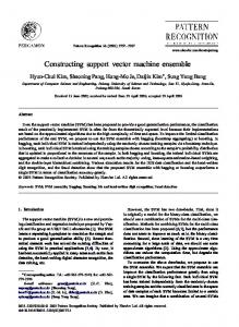
Fig. 1. Weights of training vectors in iterations. Darker points denote higher weights.

We set the sample size r to be 100 and the regularization factor γ to be 0.2. The RSVM converges in 13 iteration. In order to demonstrate the weighting procedure, we choose three iterations (iteration 1, iteration 6 and iteration 13) and plot the weights of the training vectors in Fig. 1. The darker a point appears, the higher weight the training sample has. Fig. 1 shows that how those ”important” points stand out and get higher and higher probability to be sampled. 5.2

Application in a Geographic Information System Database

We select covtype, a geographic information system database, from the UCI Repository of machine learning databases as our PRSVM applications [5]. The covtype database consists of 581,012 instances. There are 12 measures but 54 columns of data: 10 quantitative variables, 4 binary wilderness areas and 40 binary soil type variables [4]. There are totally 7 classes. We scale all quantitative variables to [0,1] and keep binary variable unchanged. We select 287831 training vectors and use our PRSVM to classify class 4 against the rest. This is a very suitable database for testing PRSVM since the database has huge number of training data and the number of SVs is limited. We set the size of working size r to be 60000, the regularization factor γ to be 0.2. We try three cases with C = 1, C = 2 and C = 4 and compare the learning time with the SVMlight in Table 1. The results show that our implementation of RSVM and PRSVM achieves comparable result with the reported fastest algorithm SVMlight , though they cannot beat SVMlight in terms of computing speed for now. However, the lack of a theoretical convergence bound makes SVMlight not always preferable.


213

Table 1. Algorithm performance comparison of SVMlight , RSVM and PRSVM Algorithm C Number of Iterations Learning Time (CPU Seconds) SV M light 1 11.7 RSVM 1 27 47.32 PRSVM 2 10 20.81 4 7 15.52

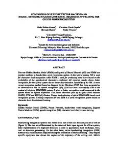
We plot the number of violators and support vectors (extremes) in each iterations in Fig. 2 to compare the performance of different number of working sites. The results show the scalability of our method. The numerical results match the theoretical result very well. 110

C=1 C=2 C=4

200

100

90

number of SVs

number of violators

250

150

100

80

70

60

50

C=1 C=2 C=4

50

40

0

0

5

10

15

20

25

number of iterations

(a) Number of Violators

30

30

0

5

10

15

20

25

30

number of iterations

(b) Number of SVs

Fig. 2. Number of violators and SVs found in each iterations of PRSVM

This figure shows the effect of adding more servers. The system with more servers will find the support vectors much faster than that with less servers.

6

Conclusions

The proposed PRSVM has the following advantages over previous works. It is able to solve general nonseparable SVM training problems. This is achieved by using KKT condition as the criterion of identifying violators and extremes. Second, our algorithm supports multiple working sets that may work parallel. Multiple working sets have more freedom than normal gradient based parallel algorithms since no synchronization and no special solver is required. Our PRSVM also has a provable and fast average convergence bound. Last, our numerical results show that multiple working sets have scalable computing advantage. The provable convergence bound and scalable results make our algorithm more preferable in some applications.

214


Further research is going to be conducted to accelerate the performance of the PRSVM. Intuitively, the weighting mechanism may be able to be improved so that the initial iterations play a more determinant role.

References 1. Ilan Adler and Ron Shamir. A randomized scheme for speeding up algorithms for linear and convex programming with high constraints-to-variable ratio. Mathematical Programming, 1993. 2. Jose Balcazar, Yang Dai, Junichi Tanaka, and Osamu Watanabe. Provably fast training algorithm for support vector machines. Proceedings of First IEEE International Conference on Data Mining (ICDM01), 2001. 3. Jose Balcazar, Yang Dai, and Osamu Watanabe. Provably fast support vector regression using random sampling. Proceedings of SIAM Workshop on Discrete Mathematics and Data Mining, April 2001. 4. Jock A. Blackard and Denis J. Dean. Comparative accuracies of artificial neural networks and discriminant analysis in predicting forest cover type from cartographic variables. Computer and Electronics in Agriculture, 24, 1999. 5. C.L. Blake and C.J. Merz. UCI repository of machine learning databases, 1998. 6. Kenneth L. Clarkson. Las vegas algorithms for linear and integer programming when the dimension is small. Proceeding of 29th IEEE Symposium on Foundations of Computer Science (FOCS’88), 1988. 7. Ronan Collobert, Samy Bengio, and Yoshua Bengio. A parallel mixture of svms for very large scale problems. In Neural Information Processing Systems, pages 633–640, 2001. 8. Tatjana Eitrich and Bruno Lang. Shared memory parallel support vector machine learning. Technical report, ZAM Publications on Parallel Applications, 2005. 9. Bernd Gartner and Emo Welzl. A simple sampling lemma: Analysis and applications in geometric optimization. Proceeding of the 16th Annual ACM Symposium on Computational Geometry (SCG), 2000. 10. Hans Peter Graf, Eric Cosatto, Leon Bottou, Igor Dourdanovic, and Vladimir Vapnik. Parallel support vector machine: The cascade svm. In Advances in Neural Information Processing Systems, 2005. 11. Thorsten Joachims. Making large-scale svm learning practical. Advances in Kernel Methods - Support Vector Learning, pages 169–184, 1998. 12. Vladimir Vapnik. The Nature of Statistical Learning Theory. Springer Verlag, New York, 1995.