Distributed Routing Algorithms for Wireless Ad Hoc Networks using d-Hop Connected d-Hop Dominating Sets Michael Q. Rieck Drake University Des Moines, Iowa 50311 USA +1 515 271 3795
[email protected]
Sukesh Pai Microsoft Corporation Mountain View, CA 94043 USA +1 650 693 3688
[email protected]
ABSTRACT This paper describes a distributed algorithm for producing a variety of sets of nodes that can be used to form the backbone of an ad hoc wireless network. The backbone produced is a d-hop dominating set, and in special cases is also d-hop connected and has a desirable “shortest path property”. d-hop dominating means that every node is within a graph distance d of some node in the set. Routing via the backbone created is also discussed. The algorithm has a constant time complexity in the sense that it is unaffected by the size of the network as long as the node degrees aren’t growing. The performances of this algorithm for various parameters are compared, and also compared with other algorithms. Keywords d-dominating set, ad hoc wireless networks, d-closure, routing algorithm. INTRODUCTION One of the important problems in ad hoc wireless networks is to find efficient routing algorithms. There are several approaches to do this. A common method is cluster-based hierarchical routing [3], [7], [8], [9]. The network is divided into several clusters and from each cluster, certain nodes are elected to be clusterheads. These clusterheads are responsible for maintaining the routing information [1], [4]. Each cluster can have one or more gateway nodes to connect to other clusters in the network. These gateway nodes ensure connectivity between all the clusters in the network. Another approach, called backbone-based routing selects certain nodes from the ad hoc network which are similar to gateway nodes. These nodes form connected dominating set and are responsible for routing within the network [5]. However, this backbone tends to be rather large. Our approach blends features of these two approaches with the intention of gaining the advantages of each. The set produced by our algorithm is not connected and does not produce a traditional backbone. It is a d-hop connected d-hop dominating set with certain properties. Let us recall that a connected dominating set is a set of vertices in a graph such that every vertex not in the set is adjacent to some vertex in the set, and the subgraph induced by the vertices in that set is connected [6]. Construction of a connected dominating set in an ad hoc net-
Subhankar Dhar San Jose State University San Jose, CA 95192 USA +1 408 924 3499 dhar
[email protected]
work is desirable because the routing process needs to only consider the subnetwork induced by this set. In this paper, we propose a distributed algorithm which can be used to produce a variety of sets of vertices which could serve as the network backbone. The sets produced are d-hop dominating, small in size and in special cases are also d-hop connected and have a certain “shortest path property”. DEFINITIONS Throughout this article, G will denote a connected graph, representing an ad hoc network. V denotes the set of all vertices in the graph G. The distance function in G will be denoted by δ. A vertex u in G is said to have eccentricity e(u) if G has a vertex v such that δ(u, v) = e(u), and for all vertices w in G, δ(u, w) ≤ e(u). The radius of G, r(G), is the minimum of the eccentricities of its vertices. Gd will denote the d-closure of G, by which we mean the graph whose vertices are the same as those of G, but which has an edge between two vertices u and v if and only if 0 < δ(u, v) ≤ d. We call a subset D of the set of vertices of G a d-hop dominating set of G if it is a dominating set for Gd , that is, if every vertex of G is within a distance d of some vertex in D. We further say that D is d-hop connected if it is connected in Gd . We say a distributed algorithm is constant-time, when the algorithm is unaffected by the size of the network as long as the vertex degrees aren’t changing. That is, the network can get bigger, but not more dense. In this case, each node will have the same amount of work to do and will do it in the same time, assuming synchronicity. RELATED WORK Minimum connected dominating sets have been used to do routing in wireless ad hoc networks. In [5], the authors use the connected dominating set on a graph to do shortest path based routing. The dominating set induces a virtual backbone of connected vertices in the graph. Since it is 1-hop connected and 1-hop dominating, the set is likely to be very big for a network with a large number of nodes. Moreover, if some node in the backbone were to fail, it
may partition the induced subgraph.
SOME NEW ALGORITHMS Altering the algorithm of Wu and Li
The Max-Min scheme for clustering nodes in a wireless ad hoc network is described in [2], which introduces the concept of d-hop dominating sets and proves that finding a minimum d-hop dominating set is NP-complete. They use the nodes selected in this set to divide the graph into a set of clusters. They assume unique IDs for each node and select a node for inclusion in the set if it has the highest ID in some d-hop neighborhood. They describe a distributed way of finding the dominating nodes by flooding the node ID information for d rounds to all the neighbors of the node. Further, they do another d rounds of flooding to determine the clusters dominated by each node in the dominating set. This algorithm is constant-time. Jie Wu and Hailan Li present a basic algorithm [10], [11] for constructing a connected dominating set in a connected graph of radius at least two. This algorithm is distributed in the sense that each node processes local information that it receives from its neighbors in order to decide whether or not it should join the dominating set, and it is constanttime. They then consider some ways to refine the basic algorithm in order to produce smaller connected dominating sets. The basic Wu-Li algorithm [11] can be characterized as follows. For each node z, the following question is asked: Does z have neighbors x and y such that x and y are not adjacent? The vertex z is then admitted to a set which we will call W uLi0 (G) if and only if the answer to this question is “yes”. It is then possible to show that W uLi0 (G) is a connected dominating set, unless G is complete (i.e. has radius one). Wu and Li then consider refining the above technique, by assuming that each vertex has a unique (perhaps randomly assigned) integer identifier. Their “Rule 1” amounts to asking a further question for each vertex z in W uLi0(G), as follows: Does z have a neighbor z 0 in W uLi0(G), whose ID is higher than that of z, and which is such that all of the neighbors of z are also neighbors of z 0 ? If so, z is deemed to be superfluous. The set W uLi1(G) consists of all the vertices from W uLi0 (G) for which the answer to the question is “no”. It too is a connected dominating set. To further reduce the size of the set, Wu and Li also introduce “Rule 2”. For each vertex z in W uLi1 (G), the following question is asked: Does z have two neighbors from W uLi1 (G), which are themselves adjacent, and which have IDs larger than that of z, and which are such that their combined neighbors include all of the neighbors of z? The set W uLi2 (G) consists of all the vertices from W uLi1 (G) for which the answer is “no”. This too can be shown to be a connected dominating set.
Let us consider the possibility of replacing “Rule 1” with a stronger condition, and refer to the resulting algorithm as altered Wu-Li. The resulting set of vertices will be denoted by D(G). Specifically, the algorithm we wish to consider proceeds as follows: 1. Consider each pair of vertices x and y which are separated by a distance 2 in G. 2. For such a pair, consider all of the common neighbors of x and y. Let E(x, y) denote the vertex among these common neighbors whose ID is largest. 3. Admit a vertex to the set D(G) if and only if it is E(x, y) for some suitable pair x and y. We will say that E(x, y) was “elected” by the pair x and y to join the set. Notice that vertices elected by altered Wu-Li are also in the set W uLi0 (G). Moreover, any vertex eliminated by Rule 1 from W uLi1(G) would not be elected to D(G). Thus D(G) ⊆ W uLi1 (G). An advantage of this approach over that of Wu and Li is the “shortest path property” described in the following theorem. This is a special case (d = 1) of Theorem 2, which is stated and proved in the next section. Theorem 1: Assume that the connected graph G has radius at least two. Then the set D(G) constructed by the altered Wu-Li algorithm is a connected dominating set. Moreover, any two vertices in G can be connected by a shortest path consisting solely of vertices from D(G) (apart from the endpoints). The d-hop connected d-hop dominating set algorithm There is a trivial way to apply the Wu-Li algorithm or altered Wu-Li algorithm in order to produce a d-hop connected d-hop dominating set for G. To do so, simply apply the Wu-Li algorithm to Gd instead of G. Then, from the standpoint of G, the resulting set is a d-hop connected d-hop dominating set. However, because the graph Gd obscures the sense of distance in G, we feel that this is not a desirable approach. By contrast, our d-hop Connected d-hop Dominating Set algorithm (d-CDS), to be proposed next, works directly with the graph G, rather than Gd , and results in a set with this desirable “shortest path property”. Moreover, we will show that this algorithm has a more efficient implementation. It is described as follows: 1. For each pair of vertices x and y satisfying δ(x, y) = d + 1, consider all of the shortest paths from x to y.
2. Consider the set of vertices that lie strictly between x and y along such a path. Let E(x, y) be the vertex in this set with the highest ID. Call this vertex E(x, y).
14
8
4
3. Construct the set Dd (G) by including all such E(x, y), and only these vertices.
6
This algorithm also has a “shortest path property”, as described in the following theorem. 13
Proof: Consider a vertex x in G. There exists a vertex y at a distance d + 1 from x. The vertex E(x, y) is in Dd (G) and is within a distance d of x. Hence Dd (G) is d-hop dominating. To show the rest, fix any two vertices u and v. Let p be a shortest path in G from u to v. Let uj denote the vertex arrived at after taking j steps along this path. (j = 0, 1, 2, ..., m, where m = δ(u, v)). Consider the vertices on p that are also in Dd (G), together with the vertices u and v. Consider the subgraph of Gd induced by this set. If this is not a path from u to v in Gd , then let i be as large as possible so that ui is either u or is in Dd (G) and is connected to u in the induced subgraph. So i < m − d. So ui+d+1 is a vertex on the path at a distance d + 1 from ui in G. Therefore, there is a path q of length d + 1 from ui to ui+d+1 which goes through an element of Dd (G), namely E(ui , ui+d+1 ). Now create another shortest path in G from u to v by replacing the subpath of p from ui to ui+d+1 with the path q. If the resulting path is still not satisfactory to establish the second claim in the theorem, then repeat the procedure. This time i will be larger. Continuing in this way, a suitable path will eventually be produced.
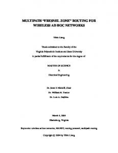
Example: Consider the example in Figure 1. The vertices here together with the solid edges constitute the graph G. By adding to this the dashed edges, the graph G2 is obtained. In this example, when the Wu-Li algorithm is applied to the graph G2 (not G), the set W uLi0 (G2 ) is found to consist of all the vertices except 2, 7, and 8. Each of these three vertices has the property that it forms a clique with its neighbors, and so does not have a pair of nonadjacent neighbors. Rule 1 eliminates vertex 5 because all of its neighbors are also neighbors of vertex 13. Rule 2 eliminates several nodes. Vertex 1 is “covered by” vertices 6 and 13 in that the combined neighbors of 6 and
15
10
2
Theorem 2: Assume that the connected graph G has radius at least d+1. Then the set Dd (G) is a d-hop connected d-hop dominating set. Moreover, any two vertices u and v from G can be connected by a shortest path (in G) with the property that the set of vertices which are on this path and also in Dd (G), together with the vertices u and v, form a connected path between u and v in the d-closure Gd .
9
3
12
1
5
11
7
Figure 1 13 include all the neighbors of 1. Moreover, vertices 1, 6 and 13 are pairwise adjacent, and of course 6 and 13 are both larger than 1. Therefore Rule 2 eliminates vertex 1. Likewise vertex 3 is covered by 6 and 12, vertex 4 is covered by 9 and 10, and vertex 11 is covered by 12 and 13. As a result, W uLi2 (G2 ) = {6, 9, 10, 12, 13, 14, 15}. So |W uLi2 (G2 )| = 7. Next consider applying altered Wu-Li to G2 . Pairs of vertices are a distance two apart in G2 if and only if they are a distance three or four apart in G. Based on this, it is not difficult to check that D(G2 ) = {1, 5, 6, 9, 10, 12, 13, 15}. So |D(G2 )| = 8. Lastly, consider 2-CDS algorithm applied to the graph G. This set consists of the nodes elected by pairs at a distance three in G, and one checks that D2 (G) = {5, 6, 9, 10, 12, 13, 15}. So |D2 (G)| = 7. Notice that this set contains the vertex 5, while W uLi2 (G2 ) does not. Also notice that the unique shortest path from 7 to 6 does not contain an intermediary node from W uLi2 (G2 ). Thus this set does not have the “shortest-path property”. By Theorem 2, the set D2 (G) must contain such a node. A further generalization The d-hop dominating set described in the previous section can be implemented in a distributed way that will be discussed in the next section. But in fact, our method can be adjusted slightly to produce even more general d-hop dominating sets. A practical motivation for this is the following. If we are willing to weaken somewhat the shortest-path property of the set Dd (G) described in Theorem 2, then it is reasonable to expect that a smaller d-hop dominating set can be produced. In this section, we will consider how this might be achieved, with implementation details left until the next section. Our general approach here is based on four non-negative integer parameters: d, e, f and g. We call it the Generalized d-hop Connected Dominating
Set (Generalized d-CDS) algorithm, and it is described as follows: 1. For each pair of vertices x and y, a distance f apart, consider all paths from x to y whose length does not exceed g. 2. Consider the set Sd,e,g (x, y) of all vertices that lie on at least one of these paths (including the endpoints), and which are within a distance d of x and a distance e of y. 3. Define Ed,e,g (x, y) to be the vertex with the largest ID among these vertices. 4. Define Dd,e,f,g (G) to be the set of such Ed,e,g (x, y) for all pairs x and y, as above. The set Dd (G) from the previous section is of course just the special case Dd,d,d+1,d+1(G) here. Also, it should be noted that in general the set Sd,e,g (x, y) and the vertex Ed,e,g (x, y) can be defined for any vertices x and y, by simply taking Sd,e,g (x, y) =
that the subpath from x to z is as short as possible, i.e. has length δ(x, z). Let w be the vertex immediately after x along this path. So w ∼ x and δ(w, z) = δ(x, z)−1 ≤ d−1. Consider the subpath from w to y that goes through z (i.e. the original path without x). This path demonstrates that z ∈ Sd−1,e,g−1 (w, y). Conversely, let w be any neighbor of x. Let z ∈ Sd−1,e,g−1 (w, y). Consider a path from w to y through z with length less than or equal to g − 1. Extend this to a path (by adding one step) from x to y. Since δ(x, z) ≤ δ(w, z) + 1 ≤ (d − 1) + 1 = d, this path demonstrates that z ∈ Sd,e,g (x, y). This establishes the first part of item 1. The second part is an immediate consequence of this. Item 2 is similarly proved, taking note however that now x is an element of Sd,e,g (x, y), but it might not be an element of any of the Sd−1,e,g−1 (w, y). Items 3 and 4 are straightforward to check.
{ z | δ(x, z) ≤ d, δ(y, z) ≤ e and δ(x, z) + δ(y, z) ≤ g },
Note that it may be assumed that g ≤ d+e, since g > d+e implies that Sd,e,g (x, y) = Sd,e,d+e (x, y).
and Ed,e,g (x, y) = max Sd,e,g (x, y), where “max” selects the vertex with the maximum ID from a set of vertices. In anticipation of the distributed algorithm in the next section for computing Dd,e,f,g (G), we offer the following observations.
Theorem 4: Fix non-negative integers d, e, f and g. Assume that the connected graph G has radius at least f , and that 0 ≤ d < f ≤ g ≤ d + e. Then the set Dd,e,f,g (G) is a d-hop dominating set.
Theorem 3: Fix non-negative integers d, e, f and g. Also, fix any two vertices x and y of G satisfying f = δ(x, y). 1. If 0 < d, 0 < g, f ≤ g and e < f , then [ Sd,e,g (x, y) = Sd−1, e, g−1 (w, y), w∼x
and so Ed,e,g (x, y) = max { Ed−1, e, g−1 (w, y) | w ∼ x } 2. If 0 < d, 0 < g, f ≤ g and f ≤ e, then [ Sd,e,g (x, y) = {x} ∪ Sd−1, e, g−1 (w, y), w∼x
and so Ed,e,g (x, y) = max{ x , max { Ed−1, e, g−1 (w, y) | w ∼ x } }. 3. If d = 0, f ≤ e and f ≤ g, or if f = 0, then Sd,e,g (x, y) is {x}, and so Ed,e,g (x, y) is x. 4. In all other cases, Sd,e,g (x, y) is empty, so that Ed,e,g (x, y) is undefined. Proof: For item 1, consider first some z ∈ Sd,e,g (x, y). This means that δ(x, z) ≤ d, δ(y, z) ≤ e, and there is a path from x to y that goes through z, and whose length does not exceed g. Since e < f , z 6= x. We may assume
The proof of this claim involves a straightforward alteration to the initial part of the proof of Theorem 2. Also, Dd,e,f,g (G) enjoys a property which approximates the shortest-path property of Dd (G). The interested reader can discover how the proof of Theorem 2 might be altered here. Of course, the initial shortest path used in the proof will no longer remain a shortest path as the path is iteratively altered. However, its growth is controlled by a constant factor. In the next section, in connection with the application of Theorem 3 as the basis of a distributed algorithm, the following lemma will also be required. Lemma 1: Fix two vertices x and y of the connected graph G. Suppose that v0 , v1 , v2 , ..., vk are vertices with x = v0 ∼ v1 ∼ v2 ∼ · · · ∼ vk = y. Then for 0 ≤ i ≤ k, δ(x, y) − i ≤ δ(vi , y) ≤ k − i. Proof: δ(x, y) ≤ δ(x, vi ) + δ(vi , y) ≤ i + δ(vi , y). This establishes the lower bound. The upper bound is immediate. A DISTRIBUTED IMPLEMENTATION The nodes in an ad hoc network, described by a connected graph G with uniquely labeled vertices (the IDs), can be coordinated in order to compute the set Dd,e,f,g (G), where
it will be assumed that 0 < d ≤ e < f ≤ g ≤ d + e. In fact, assuming that their communications can be synchronized, each node only needs to transmit g times, and simultaneously receive the corresponding messages from its neighbors, and then process these messages. Theorem 3 and Lemma 1 provide the basis for the approach to be taken for computing Dd,e,f,g (G). In addition, each node x will learn about all of the nodes within a distance g of itself, and (by means of an array next node to) for each such node, y, will also know a neighbor of x which is closer to y than x is. This can then be used to route messages locally, i.e. within a distance g, without the need to use the network backbone. In the following implementation, each message will consist of a number of ordered pairs or ordered triples of node IDs. For the first g − d rounds of message passing, ordered pairs will be transmitted. For the remaining d rounds, ordered triples will be transmitted. To simplify the discussion, given a node x in the network, the integer ID(x) will simply be denoted as “x”. Thus “x” must be read in context. The algorithm is as follows. Initialization: Each node x establishes two (possibly associative) arrays next node to and selected node, both indexed by node IDs, and containing node IDs, initially all NULL (the null node ID). Each node also maintains an (ordinary) array nodes at a distance of lists (or pointers to lists) of node IDs. These are initialized so that nodes at a distance[0] is a list consisting only of the given node x’s own ID, while the other lists are empty. After the k-th round of message passing, which could occur either in phase 1 or phase 2, the list nodes at a distance[k] will contain the nodes at a distance k from x. If y is such a node, then next node to[y] will be the ID of a neighbor of x that is closer to y than x is. Also, after the j-th round of phase 2, if a vertex y has a distance from x in the range f − d + j to g − d + j, then selected node[y] will be equal to the ID of the node Ej, e, g−d+j (x, y). Phase 1: For g − d rounds (j = 1, 2, ..., g − d), each node x broadcasts to its neighbors, a message consisting of pairs of the form: (x, s). On the j-th round x will broadcast such pairs for vertices s satisfying δ(x, s) = j − 1. These are the nodes included in the list nodes at a distance[j-1]. Upon receiving a similar pair (w, y) from one of its neighbors, a node x checks to see whether or not next node to[y] is NULL. If so, then next node to[y] is changed to w, selected node[y] is set to x, and y is added to the list nodes at a distance[j]. Phase 2: For d rounds (j = 1, 2, ...., d), each node x now broadcasts triples (x, s, t), where
1. f − d + j − 1 ≤ δ(x, s) ≤ g − d + j − 1, and 2. t = Ej−1, e, g−d+j−1 (x, s). The first of these two conditions can be managed via the array nodes at a distance. The second condition amounts to t equaling selected node[s] (as maintained by x). Note that when j = 1, the second condition reads t = E0, e, g−d (x, s), which, assuming the first condition, means t = x because δ(x, s) ≤ g − d ≤ e. Upon receiving all such triples for a given round, a node x considers collections of triples that share a common second entry y. Among these triples, let (w, y, z) denote the one with the largest third entry. Note that w must be adjacent to x. The node x now conditionally updates the entries next node to[y] and nodes at a distance[g − d + j], essentially as was done in phase 1, adjusting here to the fact that if y is a newly discovered vertex, then its distance from x is g − d + j, not j . The ultimate goal is to compute Ed,e,g (x, y) for pairs {x, y} with δ(x, y) = f . A subgoal during the j-th round of phase 2, for each node x, is to compute Ej, e, g−d+j (x, y) for relevant choices of y. Toward this end, Theorem 3 may be iteratively applied. Lemma 1, setting i to d − j and vi to the x here, implies that on the j-th round it is only necessary to consider those y that satisfy f − d + j ≤ δ(x, y) ≤ g − d + j, which can be checked via nodes at a distance (as maintained by x). Consider such a node y. If any triples having y as a second entry have been received by x from transmissions made during the previous round, then let (w, y, z) be as described earlier. Otherwise, let z = NULL. Define z 0 to be x if δ(x, y) ≤ e. Otherwise, let z 0 = NULL. Let z 00 = max{z, z 0}, where it is understood that NULL is less than any actual vertex. Using Theorem 3, it can be checked that z 00 is in fact the vertex Ej,e,g−d+j (x, y). This value is now stored in selected node[y] (as maintained by x). Once this has been done for all appropriate nodes y, the node x broadcasts a message consisting of the triples (x, y, z 00 ) for which z 00 6= NULL. After d rounds of this process, each vertex x will have stored the value Ed,e,g (x, y) in selected node[y], for each vertex y whose distance from x falls in the range from f to g. Those whose distance is f determine the set Dd,e,f,g . Once the set Dd,e,f,g has been selected, routing information can be gathered and maintained by the nodes of this set. However, every node in the network will have already learned about all of the other nodes in its g-hop neighborhood, and so local messages can easily be passed between nodes within a distance g of each other without involving
the backbone. This is achieved by means of next node to. To manage general routing through the network, a routing process that involves only the dominating nodes in the network can be implemented. Link state information can be flowed from each dominating node to other dominating nodes in its d-hop neighborhood. A dominating node can keep information about the shortest path length from it to the other dominating nodes in its d-hop neighborhood. Upon receiving link state information, each dominating node can build a weighted graph for the whole network with each link in the graph having a weight equal to the length of the shortest path between the two dominating nodes. This graph can be used to compute the shortest path between any two dominating nodes.
bounding box randomly. This changes the topology of the graph thereby simulating the movement of the nodes in an ad-hoc network. The dominating set obtained for each algorithm before and after the perturbation was compared to see how many dominating nodes changed. The sum of the number of nodes that disappeared from the previous set and the number of new nodes that appeared in the next set determines the churn produced by the perturbation. Each algorithm was run after a given graph was perturbed. This was repeated several times. Methodology
Of course, each dominating node knows about all of the nodes within a distance g of itself. When a shortest path needs to be found from a non-dominating node to another, the first node can query all the d-hop neighbors that are dominating and find the best route to the other node by comparing the path lengths returned by each after adding the cost of the shortest path to that dominating node.
For each experiment, a random disk graph was generated and measurements were taken on it. A disk graph is a graph in which a node is connected to all other nodes within a geometric radius defined for the disk graph. This radius can be seen as the coverage radius of a wireless link in the ad-hoc network. A random disk graph with n nodes was created by selecting random points in a 300 by 400 pixel 2D region. Each node is connected to all other nodes within its coverage radius. As the number of nodes in the graph increases, the degree of each node increases as there are more nodes in the vicinity of any node.
PERFORMANCE EVALUATION OF THE ALGORITHMS
Message Cost Vs Total nodes in the graph (d=3)
Performance Metrics Used 1. Message cost: All messages sent across the network for a given algorithm until completion. At every step of any algorithm, each node sends at most one message to each of its neighbors. 2. Dominating set size: The number of nodes selected in the dominating set by each algorithm. 3. Cumulative routing path length: For every pair of nodes the shortest paths through the d-hop connected dhop dominating set is determined. The length of all these shortest paths is summed for each pair of nodes for the whole graph. This determines the cumulative routing path length. 4. Churn of dominating nodes: Each algorithm was run after a given graph was perturbed slightly. In each perturbation, each node was allowed to move in a small
12000
8000
Message Cost
We implemented the Generalized d-CDS algorithm relaxing the “shortest path property” (GDCDS in the Charts, f 6= g) as well as without relaxing it (i.e, f = g, DCDS in the Charts) and compared them with basic Wu-Li with optional use of rules 1 and 2 and also the altered W uLi. The implementation was run on a single machine while simulating the distributed nature of the algorithms. Each node gathers the information it needs from its neighboring nodes and declares its results. While the above mentioned algorithms generate d-hop connected d-hop dominating sets, they were also compared to the Max-Min algorithm, which computes a d-hop dominating set.
4000
0 95
105
115
125
135
145
Total num ber of nodes GDCDS DCDS Altered WuLi
Chart 1:
MaxMin WuLi
Message Cost for d = 3
We ran the experiments on graphs with varying number of nodes to compare different algorithms for producing dhop dominating sets, as the number of nodes were changed. The algorithms considered were the Max-Min algorithm of [2], two versions of the Wu-Li algorithm (altered Wu-Li and Wu-Li with Rules 1&2 turned on) applied to the graph Gd , as well as the Generalized d-CDS algorithms without relaxing the ”shortest path property” (f = g = d+1, DCDS) and with relaxing the property (g = f + 1, f = d + 1, GDCDS). Note that all these algorithms are distributed and
Results Overall, the Generalized d-CDS algorithm performed very well compared to others in terms of the message costs and cumulative routing path lengths. The dominating set size for Generalized d-CDS was a little larger than that for Wu-Li with Rules 1 & 2 turned on. This is expected since the Generalized d-CDS may add more nodes into the set to ensure the “shortest path property”. As you can see below, when we relax the property we obtain a considerably smaller set. Chart 1 shows the message costs for each algorithm averaged over a few steps of perturbations for some graph. The DCDS algorithm has the least cost. The GDCDS has slighly higher cost than DCDS as each node gathers more information about its neighborhood than DCDS. The basic Wu-Li with Rules 1 and 2 have the same cost as the MaxMin algorithm. Both have a cost of gathering information from a d-hop neighborhood two times for each node in the graph. Altered Wu-Li has even higher cost as each node has to report what other nodes it has selected to the dominating set. Comparing Chart 1 to Chart 2, we can see as we increase the value of d, the Generalized d-CDS gets better than Wu-Li in terms of messages exchanged. The Generalized d-CDS variants for any value of f and g are upper bounded in cost by the cost for Max-Min or Wu-Li. The altered W u-Li now incurs more messages as it has to do more comparisons for each selection into the dominating set and continues to be the costliest. Chart 3 shows the the dominating set size for the various algorithms for d=3. Altered Wu-Li and DCDS have the biggest dominating sets. The GDCDS dominating set is far better than the previous ones. As we relax the ”shortest path” property constraint, we can select better nodes nodes into the dominating set that takes down the total number of nodes selected. As the node density increases, the set size remains the same for almost all the algorithms. This shows that the dominat-
Message Cost Vs Total nodes in the graph (d=4) 16000
12000 Message Cost
For every experiment, we ensure that the random graph generated has a radius sufficient to run all variants of the algorithms we consider. Specifically, we had the radius of the graphs to be at least 2d for a given value of d.
ing set is affected by the connectivity of each node. As the connectivity increase, there are more paths to be selected from and this increases the chance of a node getting into the dominating set thereby reducing the proportion of the nodes selected into the set compared to the total number of nodes in the graph.
8000
4000
0 95
105
115
125
135
145
Total num ber of nodes GDCDS DCDS Altered WuLi
Chart 2:
MaxMin WuLi
Message Cost for d = 4
MaxMin has the smallest dominating set size since it finds a d-hop dominating set that is not necessarily d-hop connected while the rest of the algorithms find d-hop connected d-hop dominating sets. Dom inating Set size Vs Total nodes in the graph (d=3) 50
Number of dominating nodes
constant-time. Hence, increasing the number of nodes has no bearing on the cost per node. But, the cost of computation and message costs depend on the degree of each node in the graph. Our intention here is to understand the behavior of the algorithms as the density of the nodes in a given area increases. In our setup, we achieve this by simply increasing the number of nodes in the same pixel 2-D region. So, when we say we increase the number of nodes or we increase the density of nodes, we imply we are increasing the average degree of each node in the graph.
40 30 20 10 0 75
95
115
135
Total nodes in the graph GDCDS DCDS Altered WuLi
Chart 3:
MaxMin WuLi
Dominating set size for d = 3
16
We evaluated variations of Generalized d-CDS algorithm relaxing the ”shortest path property” which produces a smaller dominating set size while trading off on computation costs.
Cum ulative Path length ratio (in percent)
14
% percentage
12
We are exploring cost efficient alternatives to Rule 2 in the Wu-Li algorithm. While we recognize that Rule 2 plays a very useful role in controlling the size of the set, it also sacrifices the “shortest path property”, and is costly to compute. We are also considering the idea of changing the parameters used based on dynamically obtained information about the network, like density (vertex degree).
10 8 6 4 2
ACKNOWLEDGEMENTS
0
We wish to acknowledge the assistance of Geoff Tims, Ryan Heule and Adam Whitehead for various support activities in connection with our investigations.
2
Nodes = 200
3
4
d value
Nodes = 250
5
6
Nodes = 300
Chart 4: Cumulative path length ratio comparisons Cumulative path lengths for Wu-Li with both rules is compared with the cumulative path lengths for DCDS.DCDS always find the shortest path between any two nodes. However, Wu-Li with both rules applied misses the shortest path for quite a few pair of nodes. Chart 4 shows the how worse the cumulative path lengths found by Wu-Li were as compared to the DCDS ones. The y-axis represents the ratio of the difference in the cumulative path lengths. If LW L is the cumulative path length for Wu-Li and LDCDS is the cumulative path length for DCDS, then the y-axis shows (LW L − LDCDS )/LDCDS . We see that as the value for d increases the percentage difference in the cumulative path lengths go down. This is because, more nodes are now directly connected to other nodes. As the number of nodes increases, the nodes are more connected (as discussed in Methodology section) and consequently, more nodes are directly connected to other nodes. Hence, the percentage difference decreases. CONCLUSIONS AND FUTURE WORK In this paper, we proposed a novel approach of finding a d-hop dominating set in an ad hoc wireless network that is also d-hop connected and has a certain shortest path property in some special cases. This is the basis of our routing scheme which is also very efficient from a cost perspective.
References [1] A.D. Amis and R. Prakash. L. Load-Balancing Clusters in Wireless Ad Hoc Networks. Proceedings of ASSET 2000, Richardson, Texas, March 2000. [2] A.D. Amis, R. Prakash, T.H.P. Vuong and D.T. Huynh. Max-Min D-Cluster Formation in Wireless Ad Hoc Networks. Proceedings of IEEE INFOCOM’2000, Tel Aviv, March 2000. [3] S. Bannerjee and S. Khuller. A Clustering Scheme for Higherarchical Control in Multi-hop Wireless Networks. IEEE Infocom 2001, Anchorage, Alaska, April 2001. [4] M. Chatterjee, S. Das and D. Turgut. WCA: A Weighted Clustering Algorithm for Mobile Ad Hoc Networks. Journal of Cluster Computing (Special Issue on Mobile Ad hoc Networks), Vol. 5, No. 2, April 2002, 193-204. [5] Bevan Das and Vaduvur Bharghavan. Routing in Ad-Hoc Networks Using Minimum Connected Dominating Sets. IEEE International Conference on Communications (ICC ’97), (1) 1997: 376-380. [6] S. Guha and S. Khuller. Approximation algorithms for connected dominating sets. Algorithmica, Vol 20, 1998. [7] Charles E. Perkins. Ad Hoc Networking. Addison-Wesley, Upper Saddle River, NJ, 2001. [8] R. Ramanathan and M. Streenstrup. Hierarchically-organized multihop mobile wireless networks for quality-of-service support. Mobile Networks and Applications, Vol. 3, pp. 101-119, June 1998. [9] C-K Toh. Ad Hoc Wireless Mobile Networks. Prentice Hall Inc, Upper Saddle River, NJ, 2002. [10] J. Wu and H. Li. Domination and Its Applications in Ad Hoc Wireless Networks with Unidirectional Links. Proc. of International Conference on Parallel Processing (ICPP), Aug. 2000, 189200. [11] Jie Wu and Hailian Li. A Dominating-Set-Based Routing Scheme in Ad Hoc Wireless Networks. Special issue on Wireless Networks in the Telecommunication Systems Journal, Vol. 3, 2001, 63-84.