a new routing algorithm for wireless ad hoc networks that has several ..... If no path between s and t is found, then set Ëδst := 2 · Ëδst and go to step 2. We now ...
Self-stabilizing Routing Algorithms for Wireless Ad-Hoc Networks Rohit Khot, Ravikant Poola, Kishore Kothapalli, and Kannan Srinathan Center for Security, Theory, and Algorithmic Research, International Institute of Information Technology Gachibowli Hyderabad 500 032, India {rohit a,ravikantp}@research.iiit.ac.in, {kkishore,srinathan}@iiit.ac.in
Abstract. This paper considers the problem of unicasting in wireless ad hoc networks. Unicasting is the problem of finding a route between a source and a destination and forwarding the message from the source to the destination. In theory, models that have been used oversimplify the problem of route discovery in ad hoc networks. The achievement of this paper is threefold. First we use a more general model in which nodes can have different transmission and interference ranges and we present a new routing algorithm for wireless ad hoc networks that has several nice features. We then combine our algorithm with that of known greedy algorithms to arrive at an average case efficient routing algorithm in the situation that GPS information is available. Finally we show how to schedule unicast traffic between a set of source-destination pairs by providing a proper vertex coloring of the nodes in the wireless ad hoc network. Our coloring algorithm achieves a O(Δ)–coloring that is locally distinct within the 2-hop neighborhood of any node.
1
Introduction
In this paper we consider the problem of delivering unicast messages in wireless ad-hoc networks. Unicasting is an important communication mechanism for wireless networks, and it has therefore attracted a lot of attention both in the systems and in the theory community. Unicasting can be achieved inefficiently simply by broadcasting. While unicasting in wired networks has been well understood, in wireless networks it is not an easy task. Mobile ad-hoc networks have many features that are hard to model in a clean way. Major challenges are how to model wireless communication and how to model mobility. So far, people in the theory area have mostly looked at static wireless systems (i.e. the mobile units are always available and do not move). Wireless communication is usually modeled using the packet radio network model or the even simpler unit disk graph model. In this model, the wireless units, or nodes, are represented by a graph, and two nodes are connected by an edge if they are within transmission range of each other. Transmissions of messages interfere at a node if at least two of its neighbors transmit a message at the same time. A node can only receive a message if it does not interfere with any other message. T. Janowski and H. Mohanty (Eds.): ICDCIT 2007, LNCS 4882, pp. 54–66, 2007. c Springer-Verlag Berlin Heidelberg 2007 �
Self-stabilizing Routing Algorithms for Wireless Ad-Hoc Networks
55
The packet radio network model is a simple and clean model that allows to design and analyze algorithms with a reasonable amount of effort. It assumes that the transmission range, rt , of a node is the same as its interference range, ri . In reality, the interference range of a node can be at least twice as large as its transmission range. Ignoring this fact results in inefficient algorithms that are not suitable in all situations. For example, in routing, when ri > rt , due to interference, it can take o(n) steps to find the next hop in a path. Also, when physical carrier sensing is not available if the nodes do not know any estimate of the size of the network, Ω(n) time steps are required to successfully transmit even a single message in an n node wireless network [1]. We will use a much more general model that recently appeared in [2] for designing self-stabilizing algorithms for wireless overlay networks. In this work, we show how to design efficient algorithms for routing in wireless ad hoc networks. Our algorithms work without knowledge of size or a linear estimate of size of the network and also can handle interference problems in wireless networks. Our algorithms even work under the condition that the node labels are only locally distinct. 1.1
Model and Assumptions
We review our model for wireless networks and our model for routing in this section. Wireless Communication Model. In our model, we do not just model transmission and interference range but we also model physical carrier sensing. Physical carrier sensing is used by the Medium Access Control (MAC) layer to check whether the wireless medium is currently busy. To give a short introduction, the physical carrier sensing is realized by a Clear Channel Assessment (CCA) circuit. This circuit monitors the environment to determine when it is clear to transmit. It can be programmed to be a function of the Receive Signal Strength Indication (RSSI) and other parameters. The RSSI measurement is derived from the state of the Automatic Gain Control (AGC) circuit. Whenever the RSSI exceeds a certain threshold, a special Energy Detection (ED) bit is switched to 1, and otherwise it is set to 0. By manipulating a certain configuration register, this threshold may be set to an absolute power value of t dB, or it may be set to be t dB above the measured noise floor, where t can be set to any value in the range 0-127. The ability to manipulate the CCA rule allows the MAC layer to optimize the physical carrier sensing to its needs. We assume that we are given a set V of mobile stations, or nodes, that are distributed in an arbitrary way in a 2-dimensional Euclidean space. For any two nodes v, w ∈ V let d(v, w) be the Euclidean distance between v and w. Furthermore, consider any cost function c with the property that there is a fixed constant δ ∈ [0, 1) so that for all v, w ∈ V , – c(v, w) ∈ [(1 − δ) · d(v, w), (1 + δ) · d(v, w)] and – c(v, w) = c(w, v), i.e. c is symmetric.
56
R. Khot et al.
c determines the transmission and interference behavior of nodes and δ bounds the non-uniformity of the environment. Notice that we do not require c to be monotonic in the distance or to satisfy the triangle inequality. This makes sure that our model even applies to highly irregular environments. We assume that the nodes use some fixed-rate power-controlled communication mechanism over a single frequency band. When using a transmission power of P , there is a transmission range rt (P ) and an interference range ri (P ) > rt (P ) that grow monotonically with P . The interference range has the property that every node v ∈ V can only cause interference at nodes w with c(v, w) ≤ ri (P ), and the transmission range has the property that for every two nodes v, w ∈ V with c(v, w) ≤ rt (P ), v is guaranteed to receive a message from w sent out with a power of P (with high probability) as long as there is no other node v � ∈ V with c(v, v � ) ≤ ri (P � ) that transmits a message at the same time with a power of P � . For simplicity, we assume that the ratio ρ = ri (P )/rt (P ) is a fixed constant greater than 1 for all relevant values of P . This is not a restriction because we do not assume anything about what happens if a message is sent from a node v to a node w within v’s transmission range but another node u is transmitting a message at the same time with w in its interference range. In this case, w may or may not be able to receive the message from v, so any worst case may be assumed in the analysis. The only restriction we need, which is important for any overlay network algorithm to eventually stabilize is that transmission range should have strong threshold,that is beyond the transmission range a message cannot be received any more (with high probability). This is justified by the fact that when using modern forward error correction techniques, the difference between the signal strength that allows to receive the message (with high probability) and the signal strength that does not allow any more to receive the message (with high probability) can be very small (less than 1 dB). Nodes can not only send and receive messages but also perform physical carrier sensing. Given some sensing threshold T (that can be flexibly set by a node) and a transmission power P , there is a carrier sense transmission (CST) range rst (T, P ) and a carrier sense interference (CSI) range rsi (T, P ) that grow monotonically with T and P . The range rst (T, P ) has the property that if a node v transmits a message with power P and a node w with c(v, w) ≤ rst (T, P ) is currently sensing the carrier with threshold T , then w senses a message transmission (with high probability). The range rsi (T, P ) has the property that if a node v senses a message transmission with threshold T , then there was at least one node w with c(v, w) ≤ rsi (T, P ) that transmitted a message with power P (with high probability). More precisely, we assume that the monotonicity property holds. That is, if transmissions from a set U of nodes within the rsi (T, P ) range cause v to sense a transmission, then any superset of U will also do so. Routing Model. In our model for routing, we only assume that the node labels for the source and the destination are distinct. The other nodes need labels that are only locally distinct. Our algorithms do not also require that nodes know their co-ordinate position via GPS. The routing algorithm ideally should not
Self-stabilizing Routing Algorithms for Wireless Ad-Hoc Networks
57
impose heavy storage requirement at any node. For example, space to store a constant amount of information can be assumed. Each message sent during the algorithm should also be limited to contain a constant amount of information, where the label of any node is taken as an unit of information. 1.2
Related Work
Routing algorithms for wireless ad hoc networks has been the subject of several papers, [3,4,5,6] to cite a few. Routing algorithms fall into broadly two categories namely pro-active and reactive. The pro-active algorithms maintain routing information that can be used to find a path between s and t quickly via lookup operations. Algorithms such as [7] fall under this category. The main drawback of such strategies is that they impose heavy storage overhead at the wireless nodes. Also, as the ad hoc network undergoes changes in topology, heavy recomputations may need to be performed. Reactive algorithms such as AODV[5], DSR[6], TORA[8], in contrast, rely on caching and occasional update. While the average performance of these strategies may be good, they may perform particularly bad in the worst case. For an experimental evaluation of some of these protocols see [9]. Geometric routing algorithms are also studied heavily in recent years [3,4,10,11,12]. Here, firstly it is assumed that the nodes know their actual geometric position. Secondly, a planar overlay network is also assumed to be available. The underlying geometry is used to route from s to t is done as follows. Assume that a path till node u in a path s � u � t is found. From node u, to find the next hop in the path, a greedy approach can be taken. That is, node v that is closer to t than u is selected as the next hop. This can fail in certain scenarios. In such cases, the planar overlay network is used. Here the next hop node is the node lying that is closer to t than s on the straight line connecting s and t. This is also called as face routing and one needs a planar overlay network to be able to do face routing. The work and time bounds when using this strategy are shown to be optimal in [4]. A combination of greedy algorithms and the face routing algorithms is also studied [4,13]. Most of these papers mentioned assume a Unit Disk Graph model of wireless networks. Routing algorithms based on topology control strategies such as Yao graphs [14] are also known [15]. While the topology control algorithms show the existence of energy-efficient paths, converting such existential mechanisms to constructive mechanisms for wireless networks is not easy. Vertex coloring of wireless networks is a problem that has been studied in many papers, e.g., [16,17,18,19], especially in the context of using such a coloring in a TDMA scheme. Packet scheduling in wireless networks has been studied in [18]. The results of [18] show how to use distance-2 vertex coloring to arrive at good scheduling strategies. 1.3
Our Results
As we saw in section 1.2, most of the algorithms proposed use the Unit Disk graph model which is a very weak model. We instead use a much more general
58
R. Khot et al.
and realistic model that was proposed recently in [2]. We present routing algorithm for mobile wireless ad hoc networks. That is, given a source node s and destination node t, we present algorithms to find a path between s and t. Our algorithms do not require that the spanner be a planar overlay network which is assumed in several papers on wireless routing algorithms. Further, the path returned by our algorithm is only a constant times bigger than the shortest path between s and t in the original network. We also present scheme to schedule unicast traffic in the wireless network. That is, given a set of source-destination pairs of the form {(si , ti )}i≥1 , once a path between si and ti is found, then we propose simple scheme to schedule the packet transfers in the network so that no packet is lost due to wireless interference. Our scheme relies on an O(Δ) coloring of the nodes in the network where Δ is maximum number of nodes within transmission range of a node. This coloring also has the properties that it is local and rt ⊕ ri -distinct. The rt ⊕ ri -distinctness ensures that the transmissions of nodes remain interference free. For definition of rt ⊕ ri , please see Section 2. Our algorithms are also self-stabilizing [20] which is an important property for distributed systems. Thus our algorithms can start in an arbitrary state and therefore adapt to changes in the wireless ad hoc network. We only require that the source node s and t have unique labels and the other nodes have labels that are locally distinct. The nodes should also synchronize up to some reasonably small time difference, which can be easily accomplished using GPS signals or any form of beacons. Another important feature of our algorithms is that a constant amount of storage at any node suffices. The above properties make our algorithms applicable to sensor networks without any modifications. 1.4
Structure of the Paper
The remainder of this paper is organized as follows. In Section 2, we present some preliminary definitions and assumptions which will be used by the algorithms in this paper. In Section 3, we present and analyze the wireless routing algorithm and in section 4 we propose our scheme to schedule concurrent unicast requests.
2
Preliminaries
In this section we present the notation used in the rest of the paper and then provide a review of the constant density spanner construction algorithm which we make use of in this paper. Let V be the set of nodes in the network. For any transmission range r, let the graph Gr = (V, E) denote the graph containing all edges {v, w} with c(v, w) ≤ r. Throughout this paper, rt denotes the transmission range and δuv denotes the shortest distance between u and v in Grt . Our results build on top of a distributed algorithm recently proposed for organizing the wireless nodes into a constant density spanner [2]. A constant density spanner is defined as follows: Given an undirected graph G = (V, E), a
Self-stabilizing Routing Algorithms for Wireless Ad-Hoc Networks
59
subset U ⊆ V is called a dominating set if all nodes v ∈ V are either in U or have an edge to a node in U . A dominating set U is called connected if U forms a connected component in G. The density of a dominating set is the maximum over all nodes v ∈ U of the number of neighbors that v has in U . In our context, constant density spanner is a connected dominating set U of constant density with the property that for any two nodes v, w ∈ V there are two nodes v � , w� ∈ U with {v, v � } ∈ E, {w, w� } ∈ E, and a path p from v � to w� along nodes in U so that the length of p is at most a constant factor larger than the distance between v and w in G. Our spanner protocol for Grt consists of the following 3 phases that are continuously repeated. – Phase I: The goal of this phase is to construct a constant density dominating set in Grt . This is achieved by extending Luby’s algorithm [21] to the more complex model outlined in Section 1.1. We denote by U the set of nodes in the dominating set and these nodes are also called active nodes. Since the dominating set resulting from phase I may not be connected, further phases are needed to obtain a constant density spanner. – Phase II: The goal of this phase is to organize the nodes of the dominating set of phase I into color classes that keep nodes with the same color sufficiently far apart from each other. Only a constant number of different colors is needed for this, where the constant depends on δ. Every node organizes its rounds into time frames consisting of as many rounds as there are colors, and a node in the dominating set only becomes active in phase III in the round corresponding to its color. – Phase III: The goal of this phase is to interconnect every pair of nodes in the dominating set that is within a hop distance of at most 3 in Grt with the help of at most 2 gateway nodes, using the coloring determined in phase II to minimize interference problems.We denote by G the set of gateway nodes. Each phase has a constant number of time slots associated with it, where each time slot represents a communication step. Phase I consists of 3 time slots, phase II consists of 4 time slots, and phase III consists of 4 time slots. These 11 time slots together form a round of the spanner protocol. We assume that all the nodes are synchronized in rounds, that is, every node starts a new round at the same time step. As mentioned earlier, this may be achieved via GPS or beacons. The spanner protocol establishes a constant density spanner by running sufficiently many rounds of the three phases. All of the phases are self-stabilizing. More precisely, once phase I has self-stabilized, phase II will self-stabilize, and once phase II has self-stabilized, phase III will self-stabilize. In this way, the entire algorithm can self-stabilize from an arbitrary initial configuration. For an illustration of the spanner construction, see Figure 1. It is not difficult to see that the spanner protocol results in a 5-spanner of constant density. The following result is shown in [2]:
60
R. Khot et al.
Legend:
Active Node Inactive node Gateway node Gateway Other edges
Fig. 1. Figure illustrates a constant density spanner
Theorem 1. For any desired transmission range, the spanner protocol generates a constant density spanner in O(Δ log n log Δ + log4 n) communication rounds, with high probability, where Δ is the maximum number of nodes that are within the transmission range of a node.
3
Unicasting Between s and t
In this section, we propose a new algorithm for route discovery in ad hoc networks. The algorithm works on top of the constant density spanner described in Section 2. In the following let s be a source node that intends to send a message to a target node t. We assume that s has a way to refer to node t by either the label of t or some other unique identifier. Our algorithm does not require the common assumption that a planar embedding of the original network is available. In our algorithm nodes exchange four types of messages namely RREQ, RREP, REPORT and REPLY. The RREQ, standing for Route Request, message is of the form �RREQ, s, t, d� where s and t is the source and target nodes and d is the distance over which the RREQ message is to be forwarded. Here distance is measured as distance between active nodes, thus d = 1 indicates that the RREQ message has to be forwarded to all the active nodes that are reachable from the current node by using at most 2 gateway nodes. The RREP message is of the form �RREP, s, t, flag� where flag = 1 if the current active node has t as direct neighbor and is 0 otherwise. The REPORT message is of the form �REPORT, t�, to find node t from inactive nodes. If t is found at u ,u replies with The REPLY message �REPLY, �, u� denotes u is the required node asked to find in REPORT message. We now describe the algorithm by first assuming that s knows the distance in hops to t, which is denoted by δst , where δst is the shortest distance between s and t. We call our algorithm WaveRouting algorithm and is described below. Following Section 2, each active node has 4 reserved slots for this phase. In the first slot, an RREQ are sent and in the second an RREP message may be sent. Using techniques similar to that of Phase II in Section 2, it is possible to also organize the gateway nodes into color classes so that gateway nodes that are not rt ⊕ ri apart belong to different color classes. This results in the situation that the gateway nodes also can own time slots with the property that messages sent by a gateway node during the time slot owned by it is free of interference
Self-stabilizing Routing Algorithms for Wireless Ad-Hoc Networks
61
problems. For this phase, the gateway nodes have 2 slots to send an RREQ in the first slot and an RREP in the second slot. Without loss of generality, we assume that the source node s is an active node. Otherwise, s would send an RREQ request to an active node in the transmission range of s. Each item below is a communication step. Algorithm WaveRouting(s, t, δst ) 1. If � is the source node s, then � initiates an RREQ message of the form �RREQ, �, t, δ�t � and sends the message in the first time slot. 2. If g is a gateway node that receives an RREQ message then g forwards the RREQ message to gateway nodes and active nodes that are within the rt range from g. Node g however does not decrement the counter δst . 3. If � is active and receives an RREQ message, and � �= t, then � issues a REPORT message of the form �REPORT, t�. If � = t then � prepares an RREP message and sends it in the third slot. The RREP message has the form �RREP, s, t, 1�. 4. If u is inactive and receives a REPORT message from �, and u = t then u responds with a REPLY message of the form �REPLY, �, u�. 5. If � is active and sent a REPORT message in the previous slot and did not receive any REPLY message, then � decrements the present value of δst and forwards the RREQ message. If δst is 0 after decrementing, no RREQ is sent and instead an RREP message of the form �RREP, s, t, 0� is sent signifying that � could not find a path to t. 6. If � is active and receives an RREP message and � �= s then � forwards the RREP message. If � = s and receives an RREP message with flag = 1, then a path from � to t is found. If � = s and receives an RREP message with flag = 0 then this indicates a failure. The path between s and t would simply be the reverse of the path along which successful RREP messages, that is RREP with flag = 1, arrive. This path can be located easily. The above protocol achieves the following time and work bounds. Recall that δst refers to the length of the shortest path between s and t. Lemma 1. Given a stable constant density spanner as in [2] and a source s and destination t, a path between s and t can be found in O(δst ) time steps if such a path exists. If no st–path exists, then the absence of such a path can also be reported in O(δst ) time steps. Further, the path returned has length at most 5δst . Proof. The proof follows easily from the observation that in 3 time steps, δst is decremented by 1 until δst goes to 1. It thus holds that for the entire set of RREQ and RREP messages to reach s, it takes 6δst time steps. No message is lost due to interference problems as the messages are sent by respective nodes during their own time slots.
Lemma 2. Given a stable constant density spanner as in [2] and a source s and 2 destination t,the work required to find a path between s and t is O(δst ) using the above protocol.
62
R. Khot et al.
Proof. The WaveRouting protocol requires active and gateway nodes in an area of radius δst to send and receive RREP/RREQ messages. The inactive nodes respond only to a REPORT message from an active node. Since the spanner 2 rounds construction of [2] has constant density, it holds that in an area A = πδst s, there are only O(A) active and gateway nodes. Hence the stated work bound holds.
It is not natural to assume that the source node s knows the length of the shortest path to t. However, this assumption can be easily removed. The modified algorithm is called AdaptiveWaveRouting and is described below. Algorithm AdaptiveWaveRouting(s, t) 1. δˆst = 1 2. Call WaveRouting(s, t, δˆst ). If an RREP with flag = 1 is received, stop. 3. If no path between s and t is found, then set δˆst := 2 · δˆst and go to step 2. We now show that using the Adaptive WaveRouting algorithm, if a path between s and t exists, then such a path can be found in O(δst ) time steps. Lemma 3. Given a stable constant density spanner as in [2] and a source s and destination t, a path between s and t can be found in O(δst ) time steps. Further, the path found between s and t has length at most 5δst . Proof. The AdaptiveWaveRouting protocol increases the value of δˆst by a factor of 2 until a path between s and t is found. For each value of δˆst ), the time required is O(δˆst ) by Lemma 1. Hence the total time to find a path between s and t is bounded by c(1 + 2 + 4 + . . . + δst ) ≤ 2cδst for some constant c. Hence the lemma holds.
Lemma 4. Given a stable constant density spanner as in [2] and a source s and 2 destination t,the work required to find a path between s and t is O(δst ) using the above protocol. Proof. Using arguments similar to that of Lemma 3, for each value of δˆst , the 2 work performed using the WaveRouting protocol is O(δˆst ) by Lemma 1. Hence 2 the total work performed is O(δst ).
Self-stabilization Notice that in the AdaptiveWaveRouting algorithm, no assumption is made with respect to the initial situation of the nodes in the wireless network. Since the spanner construction of [2] is known to be self-stabilizing even under adversarial behavior, we arrive at the following corollary. Lemma 5. Algorithm AdaptiveWaveRouting can be made to self-stabilize even under adversarial behavior.
Self-stabilizing Routing Algorithms for Wireless Ad-Hoc Networks
3.1
63
Extensions
Due to the lower bound shown in [13], our result is optimal in the worst case. However, our result in the current form is not comparable to the greedy or geometric routing algorithms in the average case. The advantage these algorithms have is the position information of individual nodes in the network. The position information allows the greedy algorithms to proceed in the direction of the destination with geometric algorithms coming to the rescue in the case that no intermediate node is closer to the destination than the source node. We have till now assumed that nodes do not have any information about the actual position of itself or of the destination, i.e., no GPS information was needed. But if such information is available a-priori, then we show how to combine our AdaptiveWaveRouting algorithm with that of greedy algorithms. By greedy algorithms, we mean the class of routing algorithms that forward the packet along a next hop that is geometrically closest to the destination. The idea is that as long as greedy routing is possible, we use greedy routing. Once the greedy routing scheme reaches a local minima, then we switch to AdaptiveWaveRouting. This should result in also average case optimal time-and workefficient routing algorithm. The details are omitted in this version.
4
Scheduling Unicasting Requests
Given a set of source-destination pairs {(si , ti )}i≥1 , using the AdaptiveWaveRouting algorithm, a path connecting si to ti can be found if such path exists. However, it still remains to show how to schedule the packet transmissions so that the schedule is free of wireless interference. For this, we require that a node transmitting a packet should have no other node that is within the rt ⊕ ri range also transmitting simultaneously. This problem has been studied under the assumption that the routes are available in [18]. In general, the problem can be posed as finding a valid coloring of the nodes in network such that the color of any node is unique in a rt ⊕ ri neighborhood. (In the unit disk model, this is referred to as distance-2 coloring [16]). Coloring ad hoc networks is also studied in [17] where the nodes need to know an estimate of the size of the network and the coloring achieved is not unique in rt ⊕ ri range. In this section we show that a O(Δ), distance rt ⊕ ri coloring can be achieved very easily using the spanner construction. In the context of routing, then only nodes that are in the chosen path between si and ti for some i participate in requesting a color. Thus, only nodes that need to forward the packet obtain a color. Then the color value can be associated with time slots which gives rt ⊕ ri interference free transmission slots. In the following we show how to achieve the required coloring. 4.1
Distributed Coloring of Ad Hoc Networks
In this section, we present the protocol for phase IV which results in O(Δ) coloring. In this phase, the inactive nodes request the active nodes in their neighborhood to allocate a color. The active nodes always prefix their color to the
64
R. Khot et al.
chosen color with the effect that the palettes of active nodes are locally distinct. Thus our algorithm need not have any color verification phase. In this phase, active nodes use an aCST range of ri and the inactive nodes use an aCST range of ri . Each active node maintains a counter k that is initialized to 0 and serves as an upper bound on the highest color that is allotted till now by the active node. Once all the colors till k are allotted, the active nodes updates k to 4k and colors are assigned from the range [k + 1, 4k] uniformly at random. Below we present the protocol. In the following each item represents a communication step. Inactive nodes maintain a state among {awake, asleep}. 1. If v is awake, v sends a REQUEST message of the form �REQUEST, v, color(v)� that contains the id of node v and the color of v with probability p to be determined later. color(v) is set to −1 if v is not assigned any color yet. 2. If � is active and senses or receives a collision then � sends a COLLIDE signal. If � is active and receives a REQUEST message containing the id of node v with color(v) = −1, � responds with a color message of the form �COLOR, v, color(v)� that contains an allotment of color to node v. If � senses a free channel, then � sends a FREE message of the form ��, FREE�. 3. If v is awake and receives a COLLIDE signal and v did not send a REQUEST message in the previous time slot then v goes to asleep state. If v is asleep and receives a FREE message then v goes to awake state. We now analyze the protocol and show bounds on the number of colors used, the time taken for the protocol, and also the locality property of the coloring achieved. Theorem 2. Given a stable set of active nodes that are colored in Phase II, Phase IV takes O(Δ log Δ log n) time steps with high probability to achieve an O(Δ) coloring. Proof. We prove the convergence of phase IV to a valid O(Δ) coloring in O(Δ log n log Δ) rounds after phase III has reached a stable state. Since, at that point the active nodes have reserved rounds that are distinct within the ri ⊕ ri range, we can treat the actions of active nodes independent of each other. Let (v, �) be an inactive node-active node pair such that v has to send a REQUEST message to �. Node v has at most O(Δ) inactive nodes in its interference range sending a REQUEST message to some leader node. If more than one node in awake state, with respect to �, decides to send a REQUEST message, then � will send a collision message. Since the collision message will be received by the inactive nodes, within rt range of �, awake nodes that decided not to send a REQUEST message to � in the previous slot will go to asleep state. Consider time to be partitioned into groups of consecutive rounds such that each group ends with a round where the active node � sends either an COLOR message or a FREE message. (A group ending with an COLOR message signifies a successful group and a group ending with a FREE message is a failed group).
Self-stabilizing Routing Algorithms for Wireless Ad-Hoc Networks
65
Notice that at the end of every group, whether successful or not, all the inactive nodes within the rt range of � go to awake state (by step 3 of the protocol). It is not difficult to show that the expected number of rounds in each group, successful or failed, is O(log Δ) and any group is successful with constant probability. Due to symmetry reasons any inactive node is equally likely to be send a REQUEST message in a successful group. Thus, during any successful group, for a given pair (v, �) , Pr[ v sends a REQUEST message successfully to �] ≥ 1/cΔ, for some constant c > 1. Using Chernoff bounds, for any given pair (v, �) the probability that it takes more than Δk groups so that v sends a REQUEST message to � successfully will be polynomially small for k = O(log n). It can also be shown that each group has O(log Δ) rounds not only on expectation but also with high probability. Thus any node v requires at most O(Δ log n log Δ) rounds to send a REQUEST message to � successfully w.h.p. Notice that number of colors used by the active nodes in Phase II is a constant cd1 . Also, the maximum color allotted by any active node is 4Δ. Thus the highest color any inactive node gets is 4cd1 Δ = O(Δ).
Finally, notice that any inactive node gets a color that is constant times bigger than the neighborhood of some active node in its neighborhood. Thus, the coloring achieved maintains locality with respect to the 2-neighborhood of any node. Thus, areas that are sparsely populated use lesser number of colors. This property is useful when using the coloring to get a natural TDMA scheme. We can also modify the above scheme so that only those inactive nodes that lie on some st–path only request (and receive) a colour.
5
Conclusions
In this paper we discussed a better model for wireless ad-hoc networks and presented efficient algorithms to perform unicasting in ad-hoc networks. Further challenges include handling mobility of nodes and an empirical analysis of the proposed protocols.
References 1. Jurdzinski, T., Stachowiak, G.: Probabilistic algorithms for the wakeup problem in single-hop radio networks. In: Proc. 13th International Symposium on Algorithms and Computation, pp. 535–549 (2002) 2. Onus, M., Richa, A., Kothapalli, K., Scheideler, C.: Constant density spanners for wireless ad-hoc networks. In: ACM SPAA (2005) 3. Kuhn, F., Wattenhofer, R., Zollinger, A.: Asymptotically optimal geometric mobil ad-hoc routing. In: ACM DIALM (2002) 4. Kuhn, F., Wattenhofer, R., Zhang, Y., Zollinger, A.: Geometric ad-hoc routing: of theory and practice. In: Proc. of the 22nd IEEE Symp. on Principles of Distributed Computing (PODC) (2003)
66
R. Khot et al.
5. Perkins, C.: Adhoc on demand distance vector (aodv) routing, Internet draft, draft– ietf–manet–aodv–04.txt (1999) 6. Johnson, D.B., Maltz, D.A.: Dynamic source routing in ad hoc wireless networks. In: Mobile Computing, vol. 353, Kluwer Academic Publishers, Dordrecht (1996) 7. Perkins, C., Bhagwat, P.: Highly dynamic destination-sequenced distance-vector routing (DSDV) for mobile computers. In: Proc. of ACM SIGCOMM, pp. 234–244 (1994) 8. Park, V., Corson, M.: A highly adaptive distributed routing algorithm for mobile wireless networks. In: Proceedings of IEEE Infocom, pp. 1405–1413 (1997) 9. Broch, J., Maltz, D., Johnson, D., Hu, Y., Jetcheva, J.: A performance comparison of multi-hop wireless ad hoc network routing protocols. In: Proceedings of the 4th annual ACM/IEEE International conference on Mobile computing and networking, pp. 85–97 (1998) 10. Gao, J., Guibas, L., Hershberger, J., Zhang, L., Zhu, A.: Geometric spanner for routing in mobile networks. In: MobiHoc 2001. Proc. of the 2nd ACM Symposium on Mobile Ad Hoc Networking and Computing, pp. 45–55 (2001) 11. Bose, P., Morin, P., Brodnik, A., Carlsson, S., Demaine, E., Fleischer, R., Munro, J., Lopez-Ortiz, A.: Online routing in convex subdivisions. In: International Symposium on Algorithms and Computation (ISSAC), pp. 47–59 (2000) 12. Bose, P., Morin, P., Stojmenovic, I., Urrutia, J.: Routing with guaranteed delivery in ad hoc wireless networks. ACM/Kluwer Wireless Networks 7(6), 609–616 (2001) 13. Kuhn, F., Wattenhofer, R., Zollinger, A.: Worst-case optimal and average-case efficient geometric ad-hoc routing. In: Proceedings of the 4th ACM international symposium on Mobile ad hoc networking & computing, pp. 267–278 (2003) 14. Yao, A.C.C.: On constructing minimum spanning trees in k-dimensional spaces and related problems. SIAM J. Comp. 11, 721–736 (1982) 15. Hassin, Y., Peleg, D.: Sparse communication networks and efficient routing in the plane. In: Proceedings of the ACM symposium on Principles of distributed computing, pp. 41–50 (2000) 16. Parthasarathy, S., Gandhi, R.: Distributed algorithms for coloring and domination in wireless ad hoc networks. In: Proc. of FSTTCS (2004) 17. Moscibroda, T., Wattenhofer, R.: Coloring unstructured radio networks. In: ACM SPAA, pp. 39–48 (2005) 18. Kumar, V.A., Marathe, M., Parthasarathy, S., Srinivasan, A.: End-to-end packetscheduling in wireless ad-hoc networks. In: ACM SODA, pp. 1021–1030 (2004) 19. Krumke, S., Marathe, M., Ravi, S.: Models and approximation algorithms for channel assignment in radio networks. Wireless Networks 7(6), 575–584 (2001) 20. Dijkstra, E.W.: Self stabilization in spite of distributed control. Communications of the ACM 17, 643–644 (1974) 21. Luby, M.: A simple parallel algorithm for the maximal independent set problem. In: Proc. of the 17th ACM Symposium on Theory of Computing (STOC), pp. 1–10 (1985)