May 15, 2009 - Yue M. Lu, Member, IEEE, and Martin Vetterli, Fellow, IEEE .... strategy of independently sending all coefficients of the distributed signals would ...... That is why we need to over-sample, in order to get a good approximation for.
1
Distributed Sampling of Signals Linked by Sparse Filtering: Theory and Applications Ali Hormati, Student Member, IEEE, Olivier Roy, Student Member, IEEE, Yue M. Lu, Member, IEEE, and Martin Vetterli, Fellow, IEEE
Abstract We study the distributed sampling and centralized reconstruction of two correlated signals, modeled as the input and output of an unknown sparse filtering operation. This is akin to a Slepian-Wolf setup, but in the sampling rather than the lossless compression case. Two different scenarios are considered: In the case of universal reconstruction, we look for a sensing and recovery mechanism that works for all possible signals, whereas in what we call almost sure reconstruction, we allow to have a small set (with measure zero) of unrecoverable signals. We derive achievability bounds on the number of samples needed for both scenarios. Our results show that, only in the almost sure setup can we effectively exploit the signal correlations to achieve effective gains in sampling efficiency. In addition to the above theoretical analysis, we propose an efficient and robust distributed sampling and reconstruction algorithm based on annihilating filters. Finally, we evaluate the performance of our method in one synthetic scenario, and two practical applications, including the distributed audio sampling in binaural hearing aids and the efficient estimation of room impulse responses. The numerical results confirm the effectiveness and robustness of the proposed algorithm in both synthetic and practical setups.
Index Terms Distributed sampling, finite rate of innovation, annihilating filter, iterative denoising, compressed sensing, compressive sampling, sparse reconstruction, Yule-Walker system
The authors are with the School of Computer and Communication Sciences, Ecole Polytechnique F´ed´erale de Lausanne (EPFL), CH-1015 Lausanne, Switzerland (e-mails: {ali.hormati, olivier.roy, yue.lu, martin.vetterli}@epfl.ch). Martin Vetterli is also with the Department of Electrical Engineering and Computer Sciences, University of California, Berkeley, CA 94720, USA. This work was supported by the Swiss National Science Foundation under grants 5005-67322 (NCCR-MICS) and 200020103729.
May 15, 2009
DRAFT
2
I. I NTRODUCTION Consider two signals that are linked by an unknown filtering operation, where the filter is sparse in the time domain. Such models can be used, e.g., to describe the correlation between the transmitted and received signals in an unknown multi-path environment. We sample the two signals in a distributed setup: Each signal is observed by a different sensor, which sends a certain number of non-adaptive and fixed linear measurements of that signal to a central decoder. We study how the correlation induced by the above model can be exploited to reduce the number of measurements needed for perfect reconstruction at the central decoder, but without any inter-sensor communication during the sampling process. Our setup is conceptually similar to the Slepian-Wolf problem in distributed source coding [1]–[3], which consists of correlated sources to be encoded separately and decoded jointly. While communication between the encoders is precluded, correlation between the measured data can be taken into account as an effective means to reduce the amount of information transmitted to the decoder. The main difference between our work and this classical distributed source coding setup is that we study a sampling problem and hence are only concerned about the number of sampling measurements we need to take, whereas the latter is about coding and hence uses bits as its “currency”. From the sampling perspective, our work is closely related to the problem of distributed compressed sensing, first introduced in [4] (see also [5]–[13]). In that framework, jointly sparse data need to be reconstructed based on linear projections computed by distributed sensors. In [4], the authors proposed three joint-sparsity models for distributed signals, as well as efficient algorithms for signal recovery. The first contribution of this paper is a novel correlation model for distributed signals. Instead of imposing any sparsity assumption on the signals themselves (as in [4]), we assume that the signals are linked by some unknown sparse filtering operation. Such models can be useful in describing the signal correlation in several practical scenarios (e.g., binaural audio recoding). Under the sparse-filtering model, we introduce two strategies for the design of the sampling system: In the universal strategy, we seek to successfully recover all signals, whereas in what we call the almost sure strategy, we allow to have a small set (with measure zero) of unrecoverable signals. As the second contribution of our work, we establish the corresponding achievability bounds on the number of samples needed for the two strategies mentioned above. These bounds indicate that the sparsity of the filter can be useful only in the almost sure strategy. Since the algorithms that achieve the aforementioned bounds are computationally prohibitive, we introduce, as our third contribution, a novel distributed sampling and reconstruction scheme that can recover the original signals in an efficient and robust way. As an intermediate step in the reconstruction
May 15, 2009
DRAFT
3
process, our proposed algorithm employs the annihilating filter technique to estimate the unknown sparse channel between the two signals. Several recent papers on channel estimation (e.g. [14], [15]) have also explored the sparsity of the channels, usually by using theories and techniques developed in compressed sensing. In this perspective, our proposed reconstruction algorithm can be viewed as a new approach, based on annihilating filters, to sparse channel estimation. However, we emphasize that, rather than focusing on channel estimation, our main goal is to develop efficient distributed sampling schemes based on the signal correlation provided by the sparse filtering model. The rest of this paper is organized as follows. After a precise definition of the considered model, we state in Section II a general formulation of the distributed sensing problem. In Section III-A, we demonstrate a somewhat surprising result: If one requires all possible vectors to be reconstructed perfectly, then the aforementioned correlation between the observed vectors cannot be exploited. In that case, the simple strategy of independently sending all coefficients of the distributed signals would be optimal. However, if one only considers the perfect recovery of almost all vectors, then substantial gains in sampling efficiency can indeed be achieved. We derive an achievability bound for the almost sure reconstruction in Section III-B. Since the algorithm that attains the bound has combinatorial complexity, we propose in Section IV a slightly sub-optimal, yet computationally efficient distributed algorithm based on annihilating filters [16]–[18]. Moreover, we show how the proposed method can be made robust to model mismatch using an iterative procedure due to Cadzow [19]. In Section V, we discuss several possible extensions and generalizations of the modeling and recovery algorithms proposed in this paper. Finally, Section VI presents several numerical experiments to illustrate the performance of our proposed scheme in both synthetic and practical scenarios. We conclude the paper in Section VII. II. S IGNAL M ODEL
AND
P ROBLEM S TATEMENT
A. Proposed Correlation Model Consider two signals x1 (t) and x2 (t), where x2 (t) can be obtained as a filtered version of x1 (t). In particular, we assume that x2 (t) = (x1 ∗ h)(t) ,
where h(t) =
PK
k=1
(1)
ck δ(t − tk ) is a stream of K Diracs with unknown delays {tk }K k=1 and coefficients
{ck }K k=1 . The above model characterizes the correlation between a pair of signals of interest in various
practical applications. Examples include the correlation between transmitted and received signals under multi-path propagation, with h(t) representing the unknown channel, or the spatial correlation between
May 15, 2009
DRAFT
4
signals recorded by two closely-spaced microphones in a simple acoustic environment composed of a single source. In this work, we study a finite-dimensional discrete version of the above model. As shown in Figure 1, we assume that the original continuous signal x1 (t) is bandlimited to [−σ, σ]. Sampling x1 (t) at uniform def
time interval T leads to a discrete sequence of samples xs1 [n] = x1 (nT ), where the sampling rate 1/T is set to be above the Nyquist rate σ/π . To obtain a finite-length signal, we subsequently apply a temporal window to the infinite sequence xs1 [n] and get def
x1 [n] = xs1 [n] wN [n],
for n = 0, 1, ..., N − 1,
where wN [n] is a smooth temporal window (e.g. the Kaiser window [20]) of length N . It is easy to verify that the discrete Fourier transform (DFT) of the finite sequence x1 [n] is � � 1 2πm X1 [m] = (b xs1 ⊛ w bN ) , for m = ⌊−N/2⌋ + 1, ..., ⌊N/2⌋, 2π N
(2)
where x bs1 (ω) and w bN (ω) are the discrete-time Fourier transforms of xs1 and wN , respectively, and
⊛ represents circular convolution. When N is large enough, we can omit the windowing effect, since w bN (ω)/(2π) approaches a Dirac function δ(ω) as N → ∞. It then follows from (2) that � � � � 2πm 1 2πm X1 [m] ≈ x bs1 = x b1 , N T NT
where x b1 (ω) is the continuous-time Fourier transform of x1 (t), and the equality is due to the classical sampling formula in the Fourier domain.
Applying the same procedure to x2 (t) and using (1), we have � � K X 1 2πm def X2 [m] ≈ x b2 ≈ X1 [m]H[m], where H[m] = ck e−j2πmtk /(N T ) . T NT
(3)
k=1
The above relationship implies that, like the original continuous signals x1 (t) and x2 (t), the finitelength signals x1 [n] and x2 [n] can also be approximately modeled as the input and output of a discretetime filtering operation, where the unknown filter H[m]—and in time domain h[n]—contains all the information about the original continuous filter h(t)1 . In general, the location parameters {tk } in (3) can be arbitrary real numbers, and consequently, the discrete-time filter h[n] is no longer sparse (see Figure 1 for a typical impulse response of h[n]). However, when the sampling interval T is small enough, we can assume that the real-valued delays {tk } are close enough to the sampling grid, i.e., tk /T ≈ nk for some 1
Note that in order to be unambiguous in the positions {tk }, we need to ensure that N T > max {tk }. k
May 15, 2009
DRAFT
5
x1 (t)
h(t)
...
...
...
x2 (t)
...
A/D
A/D
...
...
...
...
windowing
windowing
x1 [n] Fig. 1.
x2 [n]
h[n]
The continuous-time sparse filtering operation and its discrete-time counterpart. The two bandlimited signals x1 (t)
and x2 (t) are sampled above the Nyquist rate, followed by a smooth temporal windowing operation. Neglecting the windowing effect, we can approximately model the resulting finite-length signals x1 [n] and x2 [n] as the input and output of a discrete-time filtering operation. This filter is sparse as long as the sampling interval is fine enough.
integers {nk }. Under this assumption, the filter h[n] becomes a sparse vector with K nonzero elements, represented by h[n] =
K X
ck δ[n − nk ].
k=1
2
We will follow this assumption throughout the paper, and focus on the following model. Definition 1 (Correlation Model): The signals of interest are two vectors x1 = (x1 [0], . . . , x1 [N −1])T and x2 = (x2 [0], . . . , x2 [N − 1])T , linked to each other through a circular convolution x2 [n] = (x1 ⊛ h)[n]
for n = 0, 1, . . . , N − 1,
(4)
where h = (h[0], . . . , h[N − 1])T ∈ RN is an unknown K -sparse vector, that is, khk0 = K . def
Definition 2: The signal space X is the set of all stacked vectors xT = (xT1 , xT2 ) ∈ R2N such that its components x1 , x2 satisfy the correlation model given in Definition 1. 2
We introduce this assumption (i.e. tk /T = nk for some nk ∈ Z) mainly for the simplicity it brings to the theoretical analysis
in later parts of this paper. It is however not an inherent limitation of our work. In fact, the proposed sampling and recovery algorithm presented in Section IV can work with the case when the delays {tk }K k=1 have arbitrary real values. We demonstrate this capability in Section VI-B, where we apply the proposed algorithm in estimating acoustic room impulse responses. May 15, 2009
DRAFT
6
M1 x1
x1
A1
Dec
ˆ 1, x ˆ2 x
M2 h
Fig. 2.
x2
A2
The proposed distributed sensing setup. The ith sensor (i = 1, 2) provides an Mi -dimensional observation of the
signal xi via a non-adaptive linear transform Ai . The central decoder reconstructs the original vectors (as well as the sparse convolution kernel h) based on the received measurements.
B. Distributed Sensing and Problem Statement We consider the problem of sensing xT = (xT1 , xT2 ) in a distributed fashion, by two independent sensors taking linear measurements of x1 and x2 , respectively. The measurement matrices are fixed (i.e., they do not change with the input signals). As shown in Figure 2, suppose that the ith sensor (i = 1, 2) takes Mi linear measurements of xi . We can write y i = Ai xi ,
where y i ∈ RMi represents the vector of samples taken by the ith sensor, and Ai is the corresponding def
sampling matrix. Considering the stacked vector y T = (y T1 , y T2 ), we have y = Ax, where A1 0M1 ×N . A= 0M2 ×N A2
(5)
Note that the block-diagonal structure of A is due to the fact that x1 and x2 are sensed separately. This is in contrast to the centralized scenario in which x1 and x2 can be processed jointly and hence, the matrix A can be arbitrary. The measurements y 1 and y 2 are transmitted to a central decoder, which attempts to reconstruct the vector x through some (possibly nonlinear) mapping ψ : RM1 +M2 7→ X as b = ψ(y). x
By analogy to the Slepian-Wolf problem in distributed source coding [1], the natural questions to ask in the above sampling setup are the following: 1) What choices of sampling pairs (M1 , M2 ) will allow us to reconstruct signals x ∈ X from their samples? 2) What is the loss incurred by the distributed infrastructure in (5) over the centralized scenario in terms of the total number of measurements M1 + M2 ? May 15, 2009
DRAFT
7
3) How to reconstruct the original signals from their samples in a computationally efficient way? In what follows, we first answer the above questions in the case of universal reconstruction (Section III-A), where we want to recover all signals. We then consider almost sure reconstruction (Section III-B) in which case we allow to have a small set (with measure zero) of unrecoverable signals. In Section IV, we propose a robust and computationally efficient reconstruction algorithm based on annihilating filters. III. B OUNDS
ON
ACHIEVABLE S AMPLING PAIRS
A. Universal Recovery Let A1 and A2 be the sampling matrices used by the two sensors, and A be the corresponding blockdiagonal matrix as defined in (5). We first focus on finding those A1 and A2 such that every x ∈ X is uniquely determined by its samples Ax. Definition 3 (Universal Achievability): We say a sampling pair (M1 , M2 ) is achievable for universal reconstruction if there exist fixed measurement matrices A1 ∈ RM1 ×N and A2 ∈ RM2 ×N such that the set def � B(A1 , A2 ) = x ∈ X : ∃ x′ ∈ X with x 6= x′ but Ax = Ax′
(6)
is empty. Intuition suggests that, due to the correlation between the vectors x1 and x2 , the minimum number of samples needed to perfectly describe all possible vectors x can be made smaller than the total number of coefficients 2N . The following proposition shows that, surprisingly, this is not the case. Proposition 1: Let x1 ∈ RN and x2 ∈ RN be two signals that are related through an unknown K -sparse convolution kernel h, and sampled separately. A sampling pair (M1 , M2 ) is achievable for
universal reconstruction if and only if M1 ≥ N and M2 ≥ N . Proof: The sufficiency of the above conditions is clear. To show its necessity, let us consider two ′T stacked vectors xT = (xT1 , xT2 ) and x′T = (x′T 1 , x2 ), each following the correlation model (4). They
can be written under the form
x=
IN C
x1
IN and x′ = x′1 , C′
where C and C ′ are circulant matrices with vectors h and h′ as the first column, respectively. It holds that
May 15, 2009
IN x − x′ = C
−I N −C ′
x1 x′1
. DRAFT
8
Meanwhile, we can check that
rank
IN
−I N
C
−C ′
= rank
IN
0
C −C′ � = N + rank C − C ′ . C
When C − C ′ is full rank, the above matrix has rank 2N . This happens, for example, when C = 2I N and C ′ = I N . In that case, x − x′ can take any possible value in R2N . Consequently, if the matrix A is not full rank, we can always find two different vectors x and x′ , such that their difference x − x′ is in the null space of A, which implies that x and x′ provide the same measurement vector. Hence, a necessary condition for the set (6) to be empty is that the block-diagonal matrix A be a full rank matrix of size M × 2N , with M ≥ 2N . In particular, A1 and A2 must be full rank matrices of size M1 × N and M2 × N , respectively, with M1 , M2 ≥ N . Note that, in the centralized scenario, the full rank condition
would still require to take at least 2N measurements. Remark: As a direct consequence of the above result for universal reconstruction, each sensor can simply process its signal independently without any loss of optimality. In particular, the simple strategy of sending all observed coefficients is optimal. Moreover, it is seen in the proof of Proposition 1 that there is no penalty associated with the distributed nature of the sampling setup. In other words, the total number of measurements cannot be made smaller than 2N even if the vectors x1 and x2 can be processed jointly. The region of achievable sampling pairs is depicted as the shaded area in Figure 3. B. Almost Sure Recovery As shown in Proposition 1, universal recovery is a rather strong requirement to satisfy since we have to take at least N samples at each sensor, with no chance to exploit the existing signal correlation. In many situations, however, it is sufficient to consider a weaker requirement, which aims at finding measurement matrices that permit the perfect recovery of almost all signals from X . We will use the following definition in our discussion on the almost sure reconstruction. Definition 4 (Non-singular Probability Distribution): We say a probability distribution P over RN is non-singular if for any subset S ∈ RN with Lebesgue measure zero we have P(S) = 0. For non-singular distributions, the probability of signals living in a subspace with dimension less than N is zero. A typical example of a non-singular distribution is a jointly Gaussian distribution with a
non-singular covariance matrix. Definition 5 (Almost Sure Achievability): We say a sampling pair (M1 , M2 ) is achievable for almost sure reconstruction if there exist fixed measurement matrices A1 ∈ RM1 ×N and A2 ∈ RM2 ×N such that May 15, 2009
DRAFT
9 M2
N
2K+1 K+2 K+2 2K+1
Fig. 3.
N
M1
Shaded area: achievable sampling region for universal reconstruction. Solid line: boundary of the sampling pairs
achieved for almost sure reconstruction for K odd [any pair (M1 , M2 ) above the line is achievable]. Dashed line: boundary of the sampling pairs achieved for almost sure reconstruction by the proposed algorithm based on annihilating filters (see Section IV for details).
the set B(A1 , A2 ), as defined in (6), is of probability zero. The above definition for almost sure recovery depends on the probability distributions of the signal x1 and the sparse filter h. In our discussions in Section IV and Appendix A, we assume that the signal x1 follows a probability distribution such that the frequency components of x1 are nonzero with probability 1. Note that this condition is fairly mild and can be satisfied when x1 is drawn from any non-singular probability distribution over RN , or when x1 is sparse in a basis that is different from the standard Fourier basis. For the sparse filter h, it is sufficient to assume that, given the locations of its nonzero coefficients, the values of these coefficients are drawn from a non-singular distribution over RK . The following proposition gives an achievability bound on the number of samples needed for almost sure reconstruction. Proposition 2: Let x1 ∈ RN and x2 ∈ RN be two signals that are related through an unknown K sparse convolution kernel h, and sampled separately. A sampling pair (M1 , M2 ) is achievable for almost sure reconstruction if M1 ≥ min {K + r, N } , M2 ≥ min {K + r, N } ,
(7)
and M1 + M2 ≥ min {N + K + r, 2N } , where r = 1 + mod (K, 2). Proof: See Appendix A. Remark: Proposition 2 shows that, in contrast to the universal scenario, the correlation between the signals by means of the sparse filtering provides a large improvement in sampling efficiency in the almost sure
May 15, 2009
DRAFT
10
setup, especially when K ≪ N . We show the boundary of the above achievable region as the solid line in Figure 3. IV. A LMOST S URE R ECONSTRUCTION BASED
ON
A NNIHILATING F ILTERS
We show in the proof of Proposition 2 (see Appendix A) that the algorithm which attains the bound in (7) is combinatorial in nature and thus, computationally prohibitive. In the following, we propose a novel distributed sensing algorithm based on annihilating filters. This method, known as Prony’s method in spectral estimation, belongs to the class of model-based parametric methods for high-resolution harmonic retrieval [16], [18], [21]. This algorithm needs effectively K more measurements with respect to the achievability region for the almost sure reconstruction but can substantially reduce the reconstruction complexity to O(KN ). We start our discussion with the noiseless case. A. Noiseless Scenario The proposed distributed sensing scheme is based on a frequency-domain representation of the input signals. Let us denote by X 1 ∈ CN and X 2 ∈ CN the DFTs of the vectors x1 and x2 , respectively. The circular convolution in (4) can be expressed as X2 = H ⊙ X1 ,
(8)
where H ∈ CN is the DFT of the filter h and ⊙ denotes element-wise multiplication. Our approach consists of the following two main steps: 1) Finding the filter h by sending the first K + 1 (1 real and K complex) DFT coefficients of x1 and x2 .
2) Sending the remaining frequency indices by sharing them among the two sensors. We first show how a decoder can almost surely recover the unknown filter h using only the first K + 1 DFT coefficients of x1 and x2 . This is achieved by using the annihilating filter approach, which is widely used in harmonic retrieval applications. In what follows, we focus on the main steps of the algorithm; more details can be found in [16], [18]. The DFT coefficients of the filter h are given by H[m] =
K X
2π
ck e−j N nk m
for m = 0, 1, . . . , N − 1.
(9)
k=1
The sequence H[m] is the sum of K complex exponentials, whose frequencies are determined by the positions {nk } of the non-zero coefficients of the filter. It can be shown [16] that H[m] can be
May 15, 2009
DRAFT
11
“annihilated” by a filter A(z) of degree K whose roots are of the form e−j2πnk /N for k = 1, 2, . . . , K A(z) =
K Y
(1 − e−j2πnk /N z −1 ).
k=1
More specifically, in the spatial domain, the coefficients of this filter satisfy A[m] ∗ H[m] =
K X
A[i]H[m − i] = 0 ,
i=0
or in matrix form,
H[0]
H[−1]
···
H[1] .. .
H[0] .. .
··· .. .
H[K − 1] H[K − 2] · · ·
H[−K]
A[0]
H[−K + 1] A[1] .. .. = 0 . . . H[−1] A[K]
(10)
The above matrix is of size K × (K + 1) and is built from 2K consecutive DFT coefficients. Moreover, it can be shown to be of rank K (see Appendix B) and hence, its null space is of dimension one. Therefore, the solution can be any vector in the null-space of the above matrix. Note that, due to the conjugate symmetry property, the coefficients of the matrix in (10) can be computed as H[m] =
X2 [m] X1 [m]
and H[−m] = H ∗ [m]
(11)
provided that X1 [m] is non-zero for m = 0, 1, . . . , K . In other words, those signals x1 which have zero frequency components in the range m = 0, 1, . . . , K are unrecoverable by the annihilating filter method. However, according to our assumption on the probability distribution of x1 , such signals happen with probability 0. Once the coefficients of the annihilating filter have been obtained, it is simply a matter of computing its roots to retrieve the unknown positions {nk }. The filter weights {ck } can then be recovered by means of the linear system of equations (9). Based on the above considerations, our distributed sensing scheme can be described as follows. Both sensors send the first3 K + 1 DFT coefficients of their signals to the decoder (2K + 1 real values each). They also transmit complementary subsets4 (in terms of frequency indexes) of the remaining DFT coefficients (N − 2K − 1 real values in total). This is illustrated in Figure 4. The first K + 1 DFT coefficients allow us to almost surely reconstruct the filter h. The missing frequency components of x1 3
Note that we could also use a pass-band frequency range but in that case, we need 2K complex measurements (4K real),
since we can no longer use the complex conjugate property of the Fourier transform to build 2K consecutive frequency data from K + 1 measurements. 4
Two subsets A and B are called the complementary subsets of C if A ∩ B = ∅ and A ∪ B = C.
May 15, 2009
DRAFT
12
K +1
⌊N/2⌋ − K
X1 X2 Fig. 4.
Sensors 1 and 2 both send the first K + 1 DFT coefficients of their observations, but only complementary subsets of
the remaining frequency components.
Algorithm 1 Sensing and Recovery Based on Annihilating Filters 1: Sensors 1 and 2 send the first K +1 DFT coefficients of x1 and x2 , respectively. They also send complementary
subsets of the remaining DFT coefficients. 2: The decoder computes 2K consecutive DFT coefficients of h from (11). 3: The decoder retrieves the filter h using the annihilating filter method. 4: The decoder reconstructs x1 and x2 from (8) using h and the remaining DFT coefficients of x1 and x2 .
(resp. x2 ) are then recovered from the available DFT coefficients of x2 (resp. x1 ) using the relation (8). Note that in order to compute X1 [m] from X2 [m], the frequency component H[m] should be nonzero. This is insured almost surely under our assumption that the nonzero elements of the filter h are drawn from a non-singular distribution in RK . We summarize the proposed method in Algorithm 1. In terms of achievability, we have thus shown the following result. Proposition 3: A sampling pair (M1 , M2 ) is achievable for almost sure reconstruction using the proposed annihilating filter method if M1 ≥ min {2K + 1, N } , M2 ≥ min {2K + 1, N } ,
and M1 + M2 ≥ min {N + 2K + 1, 2N } . In contrast to the universal reconstruction, the total number of measurements can be reduced from 2N to N + 2K + 1, as depicted by the dashed line in Figure 3. Although slightly oversampled compared to the bound for the almost sure setup given in Proposition 2, we obtain substantial improvement in terms of computational efficiency, as seen in the following. The annihilating filter equation in (10) is a Yule-Walker system which is solvable in O(K 2 ) operations [22]. To find the locations of the nonzero coefficients, the annihilating filter should be factorized. The roots of the filter can be found by the Chien search algorithm in O(KN ) operations [23]. In the last step, the weights of the nonzero coefficients of the filter are obtained by solving a Vandermonde system, which requires O(K 2 ) operations [22]. Since K ≪ N , the total number of operations needed in reconstructing the sparse filter is O(KN ). May 15, 2009
DRAFT
13
Algorithm 2 Cadzow Iterative Denoising 1: Build matrix T of dimension L × (L + 1) of the form (10) from the measurements. 2: Set ǫ to be a small constant. 3: while
σK+1 σK
≥ ǫ do
4:
Enforce rank K on T by setting the L − K + 1 smallest singular values to zero.
5:
Enforce Toeplitz form on T by averaging the coefficients along the diagonals.
6: end while 7: Extract the denoised DFT coefficients from the first row and first column of T .
B. Noisy Case Noise or, more generally, model mismatch makes it difficult to directly apply the solution discussed above in practice. Adding robustness to the system requires sending additional measurements to the decoder. Our first strategy for reconstruction in the noisy scenario is to use the total least squares (TLS) approach [21] to solve the system of equations in (10). In the TLS technique, it is assumed that the observation errors are on both sides of a system of equations, instead of just on the right hand side as in the least squares approach. This approach finds the solution by minimally perturbing both sides of a system of equations, until it is satisfied. The TLS approach requires the singular value decomposition and the solution is estimated from the singular vectors [22]. In our system of equations in (10), the TLS approach consists of computing the singular value decomposition of the coefficient matrix on the right hand side and then, the solution is the singular vector which corresponds to the smallest singular value. To further improve robustness, we use an iterative method devised by Cadzow [19]. In our context, it can be summarized as follows. Sensor i transmits the first L + 1 DFT coefficients of xi (i = 1, 2) with L ≥ K . A matrix T of dimension L × (L + 1) of the form (10) is then built from these measurements.
In the noiseless case, this matrix has two key properties: (i) it has rank K (see Appendix B) and (ii) it is Toeplitz. In the noisy case, these two properties are not initially satisfied simultaneously, but can be subsequently enforced by alternatively performing the following two steps: (i) Enforce rank K by setting the L − K + 1 smallest singular values of T to zero. (ii) Enforce the Toeplitz form on T by averaging the coefficients along the diagonals. The above procedure is guaranteed to converge to a matrix which exhibits the desired properties and is closest to the initial noisy matrix in the Frobenius norm [19]. The iterations stop whenever the ratio of the (K + 1)th singular value to the K th one, σK+1 /σK , falls below a pre-determined threshold (e.g. 10−6 ). The denoised DFT coefficients are then extracted from the first row and first column, and used May 15, 2009
DRAFT
14
to solve the systems (9) and (10) using the TLS method. The method is summarized in Algorithm 2. It may happen that the sparsity parameter K is not known a priori or the sparse filter is only approximately sparse, with fast decaying entries. In these cases, it is sufficient to estimate an upperbound b b for the effective sparsity parameter5 . Then, the Cadzow denoising algorithm treats the remaining N − K K
least significant coefficients of the filter h[n] as noise. In this case, the denoising performance depends b non-significant ones. b significant coefficients with respect to the N − K on the energy of the K
V. P OSSIBLE E XTENSIONS A. Generalizing the Model In this work, we consider the correlation model which consists of sparse filters in the time domain. Using the sampling theory for signals with finite rate of innovation [17], the proposed model can be extended to cases where the unknown filters are piecewise polynomials or piecewise bandlimited functions. Moreover, the model is extendable to filters which admit a sparse representation in an arbitrary basis. In that case, one can send samples which involve random frequency measurements [5] of the sparse filter. Then, the reconstruction uses techniques based on ℓ1 minimization6 to recover the filter, with a complexity of O(N 3 ). After finding the filter, the two sensors send complementary information on the remaining frequency indices of their signals to the decoder. Finally, another possible extension of the model is to consider general linear transforms (matrices) which have a sparse representation in a matrix dictionary [24]. B. The Multiframe Setup Our discussion in this paper focuses on distributed sensing in a single frame setup, where only one “snapshot” is available for sensing and reconstruction. It is possible to consider the case where multiple consecutive frames are available and the sparse filters in different frames are inter-related through certain joint sparse models [4]. In this scenario, one can exploit the inter-relation between the underlying K -sparse filters in different frames in the sensing and recovery architecture. This allows to either reduce the total number of measurements or, make the reconstruction more robust to noise and model mismatch. In [25], we showed how to efficiently exploit the inter-relation between the sparse signals in different frames in the annihilating filter based reconstruction method. In the case of random frequency measurements followed 5
We mean the sparsity parameter that retains most of the energy of the original filter. This is a model estimation problem
which in general requires some a priori knowledge about the underlying structure which generates the sparse filter. 6
One can also use greedy algorithms like orthogonal matching pursuit [7] for reconstruction.
May 15, 2009
DRAFT
15
by the ℓ1 -based recovery method, the techniques proposed in [4] can be used to exploit redundancy across frames. VI. N UMERICAL E XPERIMENTS
AND
A PPLICATIONS
In this section, we present numerical results to demonstrate the effectiveness and robustness of the proposed sensing and recovery scheme based on annihilating filters. The simulations are divided into three parts. First, in Subsection VI-A, we run simulations on synthetic data with additive white Gaussian noise added to the sparse filter to evaluate the effect of model mismatch on the recovery algorithm. Then, in Subsection VI-B, we apply our proposed algorithm to estimate the acoustic room impulse response (RIR) generated by the image-source model [26], [27]. Finally, in Subsection VI-C, we evaluate the performance of the algorithm in a distributed audio coding application, where the goal is to localize a sound source using two hearing aid microphones.
A. Synthetic Experiments Assume that the signal x1 is of length N = 256 and the sparse filter has K = 3 or 6 non-zero coefficients. The elements of the signal x1 and the non-zero coefficients of the filter are chosen to be i.i.d. random with distribution N (0, 1). The positions of the nonzero coefficients of h are chosen uniformly from [1, · · ·, N ] at random. To evaluate the effect of model mismatch on the filter model, we add independent white Gaussian noise to all N coefficients of the filter h and get hn = h + n,
n ∼ N (0, σ 2 IN ×N ).
Then, the signal observed by the second sensor is given by xn2 = x1 ∗ hn .
We define SNR h =
khk2 . kh − hk2 n
In this simulation, we let the first sensor send the whole signal x1 , and let the second sensor transmit the first L+ 1 DFT coefficients of xn2 to the decoder, for different values of L. The decoder first estimates b , and then computes an estimate of the signal of the second the true unknown K -sparse filter h, call it h
sensor as
b b 2 = x1 ∗ h. x May 15, 2009
DRAFT
16
5
0
−5
Normalized MSE (dB)
Normalized MSE (dB)
0
−5
−10
−15
−20
−25 0
20
−15
30
40
50
−25
SNRh (dB)
128
256
384
512
768
1024
N
(a) N = 256, K = 3 Fig. 5.
TLS TLS + Cadzow denoising
−20
TLS TLS +Cadzow denoising
10
−10
(b) K = 6, L = 36, SNR h = 25 dB
Normalized MSE of the reconstructed signals. The filter coefficients are perturbed by additive white Gaussian noise.
The recovery algorithm is the annihilating filter method introduced in Section IV, with or without the Cadzow denoising step. (a) K = 3, L = 4, 7, 15 (from top to bottom) (b) K = 6, L = 36, SNR h = 25 dB and different values for the signal length N .
To evaluate the quality of the reconstruction, we calculate the normalized mean-square error (MSE) as the ℓ2 norm of the difference between the ideal noiseless signal of the second sensor x2 = x1 ∗ h and b 2 , divided by the energy of x2 , i.e., the reconstructed one, x
MSE =
kb x2 − x2 k2 . kx2 k2
The results are averaged over 50’000 realizations. Figure 5(a) shows the normalized MSE as a function of SNR h using the TLS approach, with or without the Cadzow denoising procedure introduced in Section IV. The different sets of curves correspond to different oversampling factors L = K + 1, K + 4, K + 12 (from top to bottom). We observe that the normalized MSE can be significantly reduced by sending just a few more measurements than the minimum required (i.e. 2K + 1). Besides, the gain provided by the Cadzow denoising procedure increases as the number of transmitted coefficients increases. In Figure 5(b), we show the reconstruction error as a function of the signal length N . The parameters are set to be K = 6, L = 36, SNR h = 25 dB, with N taking values from the set {128, 256, 384, 512, 768, 1024}. The results shown in the figure clearly exhibits the effectiveness of the Cadzow denoising algorithm on the reconstruction performance in the presence of model mismatch.
B. Room Impulse Response Estimation In this section, we use the proposed algorithm to estimate the room impulse response (RIR) in an acoustic environment. The same setup can also be relevant in an ultra-wideband localization scenario May 15, 2009
DRAFT
17
0.04
0.03
Amplitude
0.02
5m
0.01
0
−0.01
b
0
source 2
1.5
1.5
3
2
3m b
mic 4m
−0.02
−0.03 0
100
200
300
400
500
600
700
800
900
1000
Samples
4
(a)
(b)
Fig. 6. Synthesizing the room impulse response using the image-source model [26], [27]. (a) Room setup (b) Synthesized RIR using the image-source model.
in which one can sample the echo at much slower speed than the Nyquist rate and still get very good localization information. This experiment is a bit different from our original setup. Instead of recovering two signals x1 and x2 , our goal here is to estimate the room impulse response h by sending a signal and collecting a set of
noisy observations. In our original setup, this is equivalent to the case where the decoder has full access to the first signal x1 , and then recovers the second signal x2 and the underlying sparse filter. In this simulation, we consider two sources of noise to simulate the imperfections on both the transmitter and receiver sides. In our experiment, the acoustic room impulse response is generated by the standard image-source model (ISM) [26], [27]. This scheme provides realistic impulse responses which can be used to generate signals that would effectively be recorded in the considered environment. To produce the RIR, we used the code provided by Eric A. Lehmann, available online at http://www.watri.org.au/∼ericl. Our setup is shown in Figure 6(a). The room has dimensions xr = 5 m, yr = 4 m and zr = 3 m. The reflection coefficients of all six walls are set to 0.6. The sound source is located at coordinates xs = 2 m, ys = 2 m and zs = 1.5 m. We put the microphone at coordinates xm = 4 m, ym = 3 m and zm = 1.5 m. The speed of sound is set to c = 340 m/s and the sampling frequency is fs = 16 kHz. The impulse response is computed until the time index where its overall energy content has decreased by 20 dB, which sets the value of N to 956. Also, the RIR synthesis algorithm makes use of fractional delay filters, which allow the representation of non-integer delays for all acoustic reflections. The synthesized RIR h is shown in Figure 6(b) and consists of 150 reflections.
May 15, 2009
DRAFT
18
n2
n1 room
xt1
x1
x2
h
Decoder
(L+1) DFT Samples
b h Fig. 7.
The setup for sending and receiving signals in order to estimate the acoustic room impulse response.
The setup for sending and receiving signals is shown in Figure 7. We build the signal x1 using i.i.d. elements from the Gaussian distribution N (0, 1). In order to simulate the imperfections in sending this sequence through the loudspeaker, we add white Gaussian noise to x1 to reach an SNR(1) of 25 dB. Consequently, the transmitted signal is given by xt1 = x1 + n1 , SNR(1) =
kx1 k2 . kn1 k2
Moreover, after convolving xt1 with the RIR filter h, we add to the result another white Gaussian noise sequence n2 , which is independent of n1 and used to model the imperfections on the receiver side. Consequently, the microphone observes x2 = xt1 ∗ h + n2 ,
with SNR(2) =
kxt1 ∗ hk2 kn2 k2
set to 25 dB. In the reconstruction phase, we assume that the first sequence x1 is fully available to the recovery system (note that a noisy version of x1 is convolved with the RIR filter h). To estimate the RIR, we set K = 12 and use different oversampling factors L = 48, 84, 120 and 156 on x2 . Since the true reflection
delays are real valued, we set the root finding part in the annihilating filter method to look for roots at machine precision. In this way, our algorithm is able to find the true delays even if they do not lie on the sampling grid. The original and the reconstructed RIRs are shown in Figure 8. It can be verified visually that taking more measurements will result in better reconstruction quality. May 15, 2009
DRAFT
19
1 3
57
RIR 4 6 2
L=156
L=120
L=84
L=48
0
0
100
200
300
400
500
600
700
800
900
1000
Samples
Fig. 8. The original RIR along with the reconstructed responses with different number of measurements in a typical trial. The parameter L is set to 156, 120, 84 and 48 from top to bottom and N = 956. White Gaussian noise is added to the two signals x1 [n] and x2 [n] to get signal to noise ratio of 25 dB in each one. The recovery algorithm reconstructs K = 12 Diracs of the RIR. The numbered spikes are the 7 strongest ones considered in Table I. TABLE I T HE AVERAGE ERROR ( NORMALIZED TO THE SAMPLING PERIOD ) IN ESTIMATING THE POSITIONS OF REFLECTIONS , INDICATED BY NUMBERS IN
F IGURE 8. T HE MATCHING ALGORITHM IS BASED ON
THE
7 STRONGEST
AN EXHAUSTIVE SEARCH .
T HE BLACK SQUARE INDICATES THAT THE RESPECTIVE DELAY COULD NOT BE FOUND . T HE RESULTS ARE AVERAGED OVER 500
TRIALS .
1
2
3
4
5
6
7
L = 48
0.161
2.280
2.796
�
0.635
1.740
1.951
L = 84
0.063
0.281
0.594
0.392
0.245
0.228
1.327
L = 120
0.033
0.064
0.123
0.118
0.161
0.102
1.145
L = 156
0.028
0.040
0.081
0.082
0.083
0.086
0.669
Table I summarizes the average error (normalized to the sampling period) in estimating the positions of the 7 strongest reflections of the original RIR (see Figure 8), using the annihilating filter method. We do an exhaustive search to match the set of original and reconstructed spikes. First, we separately pick the 7 strongest among each of the two sets. Then, from the two lists, we pick two spikes that are closest May 15, 2009
DRAFT
20
in time. If their time difference is smaller than a predefined threshold (which is set to 10 samples here), they are matched and removed from the lists. This process is continued until either all the 7 strongest original spikes are matched or the minimum time difference between the remaining spikes in the two lists are more than the threshold. The errors in positions are normalized to convert the absolute error (in seconds) to the error in the number of samples. The results are averaged over 500 trials. This table clearly shows the positive effect of oversampling on the performance of the recovery algorithm. C. Binaural Hearing Aids Setup In this experiment, we consider the signals recorded by two hearing aids mounted on the left and right ears of the user [28], [29]. We assume that the signals of the two hearing aids are related through a filtering operation. We refer to this filter as binaural filter. In the presence of a single source in far field, and neglecting reverberations and the head-shadow effect [30], the signal recorded at hearing aid 2 is simply a delayed version of the one observed at hearing aid 1. Hence, the binaural filter can be assumed to have sparsity factor K = 1. In the presence of reverberations and head shadowing, the filter from one microphone to the other is no longer sparse which introduces model mismatch. Despite this model mismatch, it is assumed that the main binaural features can still be well captured with a filter having only a few non-zero coefficients. Thus, the transfer function between the two received signals should be sparse, with the main peak indicating the desired relative delay. A single sound source, located at distance d from the head of a KEMAR mannequin, moves back and forth between two angles αmin and αmax . The angular speed of the source is denoted as ω . The sound is recorded by the microphones of the two hearing aids, located at the ears of the mannequin. We want to retrieve the binaural filter between the two hearing aids at hearing aid 1, from limited data transmitted by hearing aid 2. Then, the main peak of the binaural filter indicates the relative delay between the two received signals, which can be used to localize the source. In addition to that, retrieving this binaural filter also allows the hearing aid 1 to find out the received signal at hearing aid 2. The setup is shown in Figure 9. To get the head related transfer functions (HRTF) at each position of the sound source, we used the CIPIC HRTF database7, which is a public-domain database of high-spatial-resolution HRTF measurements [31]. The database includes 2500 measurements of head-related impulse responses for 45 different subjects. In order to track the binaural impulse response, we process the received signals frame by frame in a DFT filter bank architecture [32], [33]. In this way, we calculate the near-sparse filter in each frame 7
http://interface.cipic.ucdavis.edu
May 15, 2009
DRAFT
21 α
αmax
t
d ω
αmax
αmin
αmin
elevation = 0◦ (a) Fig. 9.
(b)
Audio experiment setup. (a) A sound source travels at a distance of d meters in front of the head. It moves back and
forth with angular speed ω between the horizontal angles αmin and αmax . There are two microphones (hearing aids) at the two ears which record the received signals. (b) Angular position of the sound source with respect to time.
with a few measurements, considering it as a 1-sparse filter. We use a weighted overlap-add (WOLA) filter bank, which allows for an efficient realization of a DFT filter bank to obtain the short-time Fourier transform of the input signal. The parameters of the simulation setup is as follows. The sound source is located at the distance d = 1 meter in front of the head, at elevation 0. It travels between αmin = −45◦ and αmax = 45◦ with the angular speed of ω = 18 deg/sec. The total length of the sound is 10 seconds. In the frame by frame processing, the HRTF for the left and right ears are extracted from the database. Then, each frame of length 1024 is windowed by a Hanning window and then filtered by the impulse responses to generate the received signals for the left and right ears. The overlap between the frames is set to half of the window size. On the reconstruction phase, we use the WOLA filter bank architecture. In our implementation, the sampling frequency is set to 16 kHz. The analysis window is a Hanning window of size 896, zeropadded with 64 zeros on both sides, to give a total length of 1024 samples. In each frame, we estimate the underlying impulse response between the two ears, using the distributed algorithm presented in Section IV. Since we are interested in the relative delay between the two signals, we set K = 1, i.e., we are looking for just one Dirac. To overcome the model mismatch in the system, we send more measurements than the minimum rate and use the Cadzow’s iterative de-noising followed by the TLS method. The parameter L in our algorithm is selected from the set L = 5, 10, 15, 20, 25, which is much smaller than the frame length. This allows the left ear to localize the sound source in each frame by looking at the position of the main peak in the corresponding binaural filter. Moreover, it can reconstruct the signal received by the right ear using the frame-by-frame reconstruction approach. The original and
May 15, 2009
DRAFT
22
0.4 0.25
0.35 0.3 Reconstructed Filter
Binaural Filter
0.2
0.15
0.1
0.25 0.2 0.15
0.05 0.1 0
−0.05
0.05 0 2
4
6
8
10
12
14
16
18
20
Time (msec)
(a) Fig. 10.
2
4
6
8
10 12 Time (msec)
14
16
18
20
(b)
A typical example of the binaural filter impulse response and its one-tap sparse approximation. (a) Original version.
(b) Sparse approximation obtained by Cadzows iterative denoising + TLS algorithm. The parameters are K = 1 and L = 20. We observe that the non-zero coefficient is located at the position of the filter tap with the largest magnitude.
the reconstructed sound data are available at http://rr.epfl.ch. Note that if the angular speed of the source is small compared to the frame length, the binaural filter does not change too rapidly over several frames. Therefore, we can make the reconstruction more robust to noise and model mismatch by averaging the measurements along multiple frames. We used an exponentially weighted averaging filter, with the averaging constant equal to α = 200 msec. However, setting large values for α degrades the tracking capability of the algorithm. Figure 10 shows, as an example, the binaural filter and its approximation as a one-tap filter, estimated by the reconstruction algorithm, using L = 20 measurements. Because of the reverberations and the shadowing effects, the binaural filter is not exactly sparse. Moreover, the frame-by-frame processing further distorts the binaural filter. That is why we need to over-sample, in order to get a good approximation for the position of the main peak. Figure 11 demonstrates the localization performance of the algorithm. Figure 11(a) shows the evolution of the original binaural impulse response over time. Figures 11(b)- 11(f) exhibits the sparse approximation to the filter, obtained by the proposed algorithm, using different number of measurements. This clearly demonstrates the effect of the over-sampling factor on the robustness of the reconstruction algorithm. When multiple sources are concurrently active, the binaural filter is no longer sparse. Therefore, our scheme can not be applied directly. A possible solution is to apply the proposed scheme on a sub-band basis [34], where the assumption is that only one source is active in each sub-band. However, the conjugate symmetry property can no longer be used to obtain twice as many consecutive frequency coefficients. Moreover, the over-sampling ratio must be reduced to keep a constant total number of coefficients. We
May 15, 2009
DRAFT
23
0.8
0.8
2
0.6
1.5
0
−0.4
0.4 1
0.2
0.5
0 −0.2
0
−0.4
−0.6
−1 6
8
−1
10
0
2
4
Time (s)
6
8
0
4
1.5
1.5
0
−0.4
0.4 1
0.2
0.5
0 −0.2
0
−0.4
10
−0.2
0 −0.5
−0.6
−1 8
0.5
0
−0.5 −0.6
6
1
0.2
−0.4
−0.5 −0.6
delay (msec)
−0.2
delay (msec)
0
2
0.6
0.4
0.5
10
0.8
2
1.5 0.4 1
8
(c) L = 10
0.6
0.2
6 Time (s)
0.8
2
0.6
4
2
(b) L = 5
0.8
delay (msec)
−1
10
Time (s)
(a) Original
2
0 −0.5
−0.6 4
0.5
0 −0.2
−0.5
−0.6 2
1
0.2
−0.4
−0.5
−1 0
2
Time (s)
4
6
8
10
−1 0
2
4
Time (s)
(d) L = 15 Fig. 11.
delay (msec)
0.5
0 −0.2
delay (msec)
delay (msec)
0.2
0
1.5
0.4 1
2
0.6
1.5 0.4
0
0.8
2
0.6
6
8
10
Time (s)
(e) L = 20
(f) L = 25
Tracking the binaural impulse response with a 1-tap filter using different number of measurements. The quality
of estimating the main delay improves significantly by increasing the number of measurements. Each column in the image corresponds to the binaural impulse response at the time mentioned on the x axis. (a) Original binaural filter. (b)-(f) Tracking the evolution of the main peak with different values of the oversampling factor L. TABLE II S UMMARY OF THE MAIN RESULTS sparsity
measurements
complexity
universal
K
2N
O(1)
almost sure
K
N + K + 1 + mod(K, 2)
combinatorial
annihilating filter
K
N + 2K + 1
O(KN )
leave this for future work. VII. C ONCLUSIONS We investigated the task of recovering distributed signals at a central decoder based on linear measurements obtained by distributed sensors, using a fixed linear measurement structure. Our main focus was on the scenario where the two signals are related through a sparse time-domain filtering operation. Under this model, we proposed universal and almost sure reconstruction strategies. We derived the achievability bounds on the minimum number of samples needed in each strategy and showed that, for universal May 15, 2009
DRAFT
24
recovery, one can not use the sparsity of the filter to reduce the number of measurements. On the other hand, by means of a computationally demanding recovery algorithm, the number of measurements in the almost sure setup is decreased effectively by N −K . Since K ≪ N , this is about a two times reduction in the number of measurements. To overcome the high complexity of the recovery algorithm, we proposed a slightly sub-optimal yet robust distributed sensing and recovery scheme based on annihilating filters. The proposed approach needs effectively K more measurements compared to the theoretical achievability bound but its complexity is of O(KN ). The results are summarized in Table II. Our future work will focus on pursuing more practical applications of the proposed algorithm, e.g., in binaural hearing aids [28], [29]. A PPENDIX A T HE ACHIEVABILITY B OUND
FOR
A LMOST S URE R ECONSTRUCTION
The goal of this appendix is to show the achievability result for the almost sure reconstruction as stated in Proposition 2. To this end, we first state some definitions and lemmas. Definition 6 (Spark [35]): The spark of a matrix A, denoted as S(A), is defined as the largest integer L, such that every sub-group of L columns from A are linearly independent.
The following lemma shows that, using a measurement matrix with Spark at least K + 1, we can almost surely reconstruct a K -sparse signal with only K + 1 measurements. Our proof follows the main ideas of the proof sketched in [4], but with a few additional details. Lemma 1 (Sparse Reconstruction): Let h ∈ RN be a K -sparse vector with the non-zero coefficients chosen from a non-singular distribution in RK . Furthermore, let A be a matrix with N columns, satisfying S(A) ≥ K + 1. Then almost surely, we can reconstruct the sparse vector h from the measurements y = Ah.
Proof: Assume, without loss of generality, that the non-zero coefficients of h lie on the first K indices I = {1, 2, . . . , K}. The measurement vector y lives in the span of the columns of A indexed by I ; we denote these columns by AI and define AI , Span {AI }.
The combinatorial search algorithm goes through all the possible
N� K
subspaces and checks to which one
the measurement vector y belongs. Let I ′ be any other set of indices different from I with cardinality K . Since S(A) ≥ K + 1, the dimension of the sum of the two subspaces AI and AI ′ satisfies
dim(AI∪I ′ ) ≥ K + 1.
May 15, 2009
(12)
DRAFT
25
It can be easily verified that dim(AI∪I ′ ) = dim(AI ) + dim(AI ′ ) − dim(AI ∩ AI ′ ). Meanwhile, since dim(AI ) = dim(AI ′ ) = K , we have dim(AI ∩ AI ′ ) < K. Since the columns of AI are linearly independent and the non-zero elements of h have a non-singular probability distribution, it is easy to show that any low dimensional subspace of AI have probability zero. To see this, take any low dimensional subspace S ′ of AI , and let v be a nonzero vector in the null space of S ′ . We have v T AI hI = 0.
This shows that the non-zero elements of h which generate the subspace S ′ live in span⊥ {v}, a proper subspace of RK . Since the non-zero elements of h have a non-singular probability distribution, these nonzero elements have probability zero which in turn, indicates that the subspace S ′ have probability zero. Therefore, this intersection set of dimension less than K has total probability zero in AI . Since the number of subspaces are finite, the total probability of the set of points in AI which also live in any other subspace AI ′ is zero. Thus, there is a one-to-one relationship between the measurements y and � N the sparse vector h almost surely. In general, the recovery algorithm should search through all K
possible subspaces and check to which one the measurement vector y belongs. Therefore, the recovery algorithm is combinatorial in nature and computationally prohibitive. Note that if the filter h lies in the intersection of two subspaces (which has probability zero under the conditioned discussed), the filter is not recoverable uniquely. Now we are ready to prove the achievability result stated in Proposition 2. We divide the sensing and recovery architecture into two parts: I. The two sensors send frequency measurements to the decoder, necessary to find the underlying K sparse filter h. For fixed values of N and K , the structure of this part does not change by choosing different values for the number of measurements M1 and M2 in the achievability region. II. The sensors transmit complementary subsets of the DFT coefficients necessary to construct the two signals x1 and x2 . The sensors adjust their share on this part of linear measurements in order to reach the required rates M1 and M2 . We show the results of Proposition 2 in two separate situations, corresponding to whether K is an odd or even number. May 15, 2009
DRAFT
26
(a) K is odd: In part I, define the matrix M of size ( K+1 2 + 1) × N as 1 i = j, j ∈ {1, . . . , K+1 + 1} 2 M (i, j) = 0 otherwise. (I)
(I)
The two sets of measurements in part I, denoted as y 1 and y 2 , are given by (I)
y 1 = M F x1 (I) y2
(13)
= M F x2 ,
in which F is the DFT matrix of size N × N . The number of real measurements in (13) is K + 2 for each sensor, composed of 1 real DC component plus (K +1)/2 complex frequency components. In order to reconstruct the sparse filter h, the central decoder computes the consecutive frequency K+1 components of h in the index range N = {− K+1 2 , . . . , 2 }. This is done by dividing the two sets
of measurements in (13) index by index and making use of the complex conjugate property of the Fourier transform of real sequences. Note that this division is allowed as long as the denominator is not zero. Since a zero frequency component forces x1 to lie on a hyperplane in RN , the frequency components are nonzero almost surely for the signal x1 drawn from a non-singular distribution in RN (More precisely, we only require that the frequency components of x1 be non-zero in the range N ). In the matrix form, we obtain H = W h,
where H is the Fourier transform of h in the range given by N . The matrix W is a complex valued generalized Vandermonde system [36] of size (K + 2) × N which consists of K + 2 consecutive rows of the DFT matrix, corresponding to the indices in the set N , i.e., Wpq = e−j2π(p−
K+1 −1)(q−1)/N 2
, p ∈ {1, . . . , K + 2} q ∈ {1, . . . , N }.
Thus, by the properties of generalized Vandermonde matrices, we get S(W ) = K + 2.
Note that, by assumption, the non-zero elements of h satisfy a non-singular distribution in RK . (I)
(I)
Therefore, by Lemma 1, it is possible to find the K -sparse filter h from y 1 and y 2 almost surely. In the second part of the sensing and recovery architecture, the sensors send complementary subsets of the remaining frequency information of their signals x1 and x2 to the decoder. By having access
May 15, 2009
DRAFT
27
to the frequency information of one of the signals xi , i = 1, 2, the decoder uses the point-wise relationship X2 [m] = X1 [m]H[m],
(14)
to get the frequency content of the other sequence, with the help of the known filter h. Note that since the non-zero elements of h satisfy a non-singular distribution in RK , the frequency components of the filter are all non-zero almost surely. Therefore, it is possible to find X2 [m] from X1 [m] or vice-versa. The two sensors share the rest of the frequency indices to reach any point
on the achievability region. Note that (14) also allows the decoder to calculate the real (imaginary) part of X2 [m] by knowing the imaginary (real) part of the other sequence X1 [m] and vice-versa. This is achieved by equating the real and imaginary parts in (14) and solving a linear system of equations. In this way, each sensor sends K + 2 real measurements in part I for the decoder to find the underlying sparse filter h almost surely. Moreover, in part II, the sensors send complementary information to the decoder. This indicates that the sensors can choose the sampling pairs given by K + 2 ≤ M1 ≤ N and M2 = K + 2 + N − M1 . Therefore, the algorithm described above attains
any point on the achievability region given in Proposition 2. (b) K is even: The same measurement and reconstruction techniques apply. In this case, however, we are able to find the K -sparse filter h from K + 1 real measurements, instead of K + 2. This corresponds to the matrix M of size ( K2 + 1) × N , given by 1 i = j, j ∈ {1, . . . , K + 1} 2 M (i, j) = 0 otherwise.
Therefore, when K is even, we have
M1 ≥ min {K + 1, N } , M2 ≥ min {K + 1, N } ,
and M1 + M2 ≥ min {N + K + 1, 2N } . A PPENDIX B D ERIVATION
OF
T HE R ANK P ROPERTY
We investigate the rank property of the Toeplitz matrices constructed by a signal which is composed by a sum of K exponentials. We show that whenever the number of rows and columns of this matrix is larger than or equal to K , its rank is K . May 15, 2009
DRAFT
28 K Consider a sequence h of length N with K non-zero coefficients {αi }K i=1 at positions {ni }i=1 . The ′
L + L + 1 consecutive frequency samples of h (starting from index P − L) are given by H[m] =
K X
αi ωim , m = (P − L), . . . , (P + L ), ′
i=1
where ωi ,
e−j2πni /N
′
′
and L, L ≥ K − 1. We build the Toeplitz matrix H of size (L + 1) × (L + 1) as H[P ] H[P − 1] ··· H[P − L] H[P + 1] H[P ] · · · H[P − L + 1] . H= .. .. .. .. . . . . ′ ′ ′ H[P + L ] H[P + L − 1] · · · H[P + L − L]
To show that the rank of H is K , we can write it as the product H =UCV,
where the three matrices are given by
ω1P
ω2P
P ωK
···
P +1 ω1 ω2P +1 · · · ′ U (L +1)×K = .. .. .. . . . ′ ′ ω1P +L ω2P +L · · · α 0 ··· 0 1 0 α2 · · · 0 C K×K = .. .. . . .. . . . . 0 0 · · · αK
P +L ωK
and
V K×(L+1)
=
P +1 ωK .. . ′
,
1
ω1−1
···
ω1−L
1 .. .
ω2−1
··· .. .
ω2−L .. .
−1 1 ωK ···
−L ωK
.. .
.
The matrices U and V are Vandermonde matrices of rank K . Therefore, since the diagonal elements of C are nonzero, the matrix H is of rank K .
May 15, 2009
DRAFT
29
R EFERENCES [1] D. Slepian and J. K. Wolf, “Noiseless coding of correlated information sources,” IEEE Trans. Inf. Theory, vol. 19, pp. 471– 480, Jul. 1973. [2] T. Berger, “Multiterminal source coding,” Lectures Notes Presented at CISM Summer School on the Information Theory Approach to Communications, Jul. 1977. [3] Y. Oohama, “Gaussian multiterminal source coding,” IEEE Trans. Inf. Theory, vol. 43, pp. 1912–1923, Nov. 1997. [4] D. Baron, M. B. Wakin, M. F. Duarte, S. Sarvotham, and R. G. Baraniuk, “Distributed compressed sensing,” Tech. Rep. ECE-0612, Electrical and Computer Engineering Department, Rice University, Dec. 2006. [5] E. J. Cand`es, J. Romberg, and T. Tao, “Robust uncertainty principles: Exact signal reconstruction from highly incomplete frequency information,” IEEE Trans. Inf. Theory, vol. 52, pp. 489–509, Feb. 2006. [6] D. L. Donoho, “Compressed sensing,” IEEE Trans. Inf. Theory, vol. 52, pp. 1289–1306, Apr. 2006. [7] J. A. Tropp and A. Gilbert, “Signal recovery from random measurements via orthogonal matching pursuit,” IEEE Trans. Inf. Theory, vol. 53, pp. 4655–4666, Dec. 2007. [8] E. J. Candes and T. Tao, “Near optimal signal recovery from random projections: Universal encoding strategies?,” IEEE Trans. Inf. Theory, vol. 52, pp. 5406–5425, Dec. 2006. [9] D. L. Donoho, M. Elad, and V. N. Temlyakov, “Stable recovery of sparse overcomplete representations in the presence of noise,” IEEE Trans. Inf. Theory, vol. 52, pp. 6–18, Jan. 2006. [10] W. Wang, M. J. Wainwright, and K. Ramchandran, “Information-theoretic limits on sparse signal recovery: Dense versus sparse measurement matrices,” Tech. Rep. 754, UC Berkeley, May 2008. [11] W. Bajwa, J. Haupt, A. Sayeed, and R. Nowak, “Compressive wireless sensing,” in Proc. Int. Conf. on Information Processing in Sensor Networks, pp. 134–142, Apr. 2006. [12] M. Rabbat, J. Haupt, A. Singh, and R. Nowak, “Decentralized compression and predistribution via randomized gossiping,” in Proc. Int. Conf. on Information Processing in Sensor Networks, pp. 51–59, Apr. 2006. [13] W. Wang, M. Garofalakis, and K. Ramchandran, “Distributed sparse random projections for refinable approximation,” in Proc. Int. Conf. on Information Processing in Sensor Networks, pp. 331–339, Apr. 2007. [14] W. U. Bajwa, J. Haupt, G. Raz, and R. Nowak, “Compressed channel sensing,” in Proc. 42nd Annu. Conf. Information Sciences and Systems (CISS 08), (Princeton, NJ), pp. 5–10, Mar. 2008. [15] J. Paredes, G. Arce, and Z. Wang, “Ultra-wideband compressed sensing: Channel estimation,” IEEE Journ. Sel. Top. Sig. Proc, vol. 1, pp. 383–395, Oct. 2007. [16] P. Stoica and R. Moses, Introduction to Spectral Analysis. Englewood Cliffs, NJ: Prentice-Hall, 2005. [17] M. Vetterli, P. Marziliano, and T. Blu, “Sampling signals with finite rate of innovation,” IEEE Trans. Signal Process., vol. 50, pp. 1417–1428, Jun. 2002. [18] T. Blu, P. Dragotti, M. Vetterli, P. Marziliano, and L. Coulot, “Sparse sampling of signal innovations,” IEEE Signal Process. Mag., vol. 25, no. 2, pp. 31–40, 2008. [19] J. A. Cadzow, “Signal enhancement – A composite property mapping algorithm,” IEEE Trans. Acoust., Speech, Signal Process., vol. 36, pp. 49–67, Jan. 1988. [20] A. V. Oppenheim and R. W. Schafer, Discrete-Time Signal Processing. Englewood Cliffs, NJ: Prentice-Hall, 1989. [21] B. Rao and K. Arun, “Model based processing of signals: A state space approach,” Proc. IEEE, vol. 80, pp. 283–309, Feb. 1992. [22] G. H. Golub and C. F. Van Loan, Matrix Computations. Baltimore, MD: Johns Hopkins Univ. Press, 1989.
May 15, 2009
DRAFT
30
[23] R. T. Chien, “Cyclic decoding procedure for the Bose-Chaudhuri-Hocquenghem codes,” IEEE Trans. Inf. Theory, vol. 10, pp. 357–363, Oct. 1964. [24] G. E. Pfander, H. Rauhut, and J. Tanner, “Identification of matrices having a sparse representation,” IEEE Trans. Signal Process., vol. 56, pp. 5376–5388, Nov. 2008. [25] A. Hormati and M. Vetterli, “Distributed compressed sensing: Sparsity models and reconstruction algorithms using annihilating filter,” in Proc. ICASSP, pp. 5141–5144, Apr. 2008. [26] J. B. Allen and D. A. Berkley, “Image method for efficiently simulating small-room acoustics,” J. Acoust. Soc. Am., vol. 65, pp. 943–950, Apr. 1979. [27] E. A. Lehmann and A. M. Johansson, “Prediction of energy decay in room impulse responses simulated with an imagesource model,” J. Acoust. Soc. Am., vol. 124, pp. 269–277, Jul. 2008. [28] O. Roy, Distributed Signal Processing for Binaural Hearing Aids. PhD thesis, Ecole Polytechnique F´ed´erale de Lausanne, Switzerland, Oct. 2008. [29] O. Roy and M. Vetterli, “Rate-constrained collaborative noise reduction for wireless hearing aids,” IEEE Trans. Signal Process., vol. 57, no. 2, pp. 645–657, 2009. [30] J. Blauert, Spatial Hearing: The Psychophysics of Human Sound Localization. Cambridge, MA: MIT Press, 1997. [31] V. R. Algazi, R. O. Duda, D. M. Thompson, and C. Avendano, “The CIPIC HRTF database,” in Proc. IEEE WASPAA, vol. 100, pp. 99–102, Oct. 2001. [32] R. E. Crochiere and L. R. Rabiner, Multirate Digital Signal Processing. Englewood Cliffs, NJ: Prentice-Hall, 1983. [33] M. Vetterli and J. Kovaˇcevi´c, Wavelets and Subband Coding. Englewood Cliffs, NJ: Prentice-Hall, 1995. [34] C. Faller, Parametric Coding of Spatial Audio. PhD thesis, Ecole Polytechnique F´ed´erale de Lausanne, Switzerland, Jul. 2004. [35] D. L. Donoho and M. Elad, “Maximal sparsity representation via ℓ1 minimization,” in Proc. Natl. Acad. Sci., vol. 100, pp. 2197–2202, Mar. 2003. [36] F. R. Gantmacher, Matrix Theory. Providence, RI: AMS Chelsea Publishing, 2000.
May 15, 2009
DRAFT