Distributed streaming and compression architecture for point clouds ...

Bachelor thesis Björn Eberhardt Distributed streaming and compression architecture for point clouds from mobile devices

Fakultät Technik und Informatik Studiendepartment Informatik

Faculty of Engineering and Computer Science Department of Computer Science

Björn Eberhardt Distributed streaming and compression architecture for point clouds from mobile devices

Bachelorarbeit eingereicht im Rahmen der Bachelorprüfung im Studiengang Bachelor of Science Angewandte Informatik am Department Informatik der Fakultät Technik und Informatik der Hochschule für Angewandte Wissenschaften Hamburg Betreuende Prüferin: Prof. Dr. Birgit Wendholt Zweitgutachter: Prof. Dr. Thomas Schmidt Eingereicht am: 11. September 2015

Björn Eberhardt

Thema der Arbeit Verteilte Streaming- und Kompressionsarchitektur für Punktwolken von mobilen Geräten Stichworte Punktwolkenübertragung, Tiefenbildübertragung, Übertragung, Punktwolken, Tiefenbilder, Kompression, Datenkompression, Kompressionsalgorithmen, Performanz, Latenz, Verfahren, Structure Sensor, drahtlos, mobil, stationär, System, Handgestenerkennung, Objekterkennung, auslagern, Virtuelle Realität, Gemischte Realität, Tiefensensor, Wearable, Client-ServerArchitektur, Java, Graustufenbilder, 16-bit, Schnittstellen, zeitkritisch, Android, Architektur, Geschwindigkeit, Jpeg-LS, Deflate, BZip2, Snappy, Samsung Galaxy Tab 2, P5110, QVGA, Benutzerinteraktion, Parallelisierung Kurzzusammenfassung Diese Arbeit stellt eine verteilte zweistufige Streaming- und Kompressionsarchitektur für Punktwolken von mobilen Android-Geräten vor. Tiefenbilder eines am mobilen Gerät angeschlossenen Structure-Sensors werden effizient auf stationäre Systeme übertragen und anschließend in Punktwolken umgewandelt und weiterverteilt. Das Verfahren eignet sich, um intensive Berechnungen wie Handgesten- und Objekterkennung auf leistungsfähigere Geräte auszulagern. Dies wird zum Beispiel für Szenarien mit virtueller und gemischter Realität benötigt, da der Sensor am Körper getragen werden kann. Es wird eine effiziente Client-Server-Architektur in Java vorgestellt. Die Sensordaten werden als Graustufenbilder mit 16-bit Farbtiefe übertragen. Auf dem stationären System werden Punktwolken berechnet und über Schnittstellen weiterverteilt. Entwurfsmuster, die sich für die Aufgabe der zeitkritischen Übertragung großer Datenmengen eignen, werden angepasst und eingesetzt. Bisherige Lösungen boten keine zufriedenstellende Integration in Android-Systeme. Verschiedene Datenkompressionsalgorithmen werden in diese Architektur integriert, und die Geschwindigkeit und Latenz unter realen Bedingungen gemessen. Verglichen wurden Jpeg-LS, Deflate, BZip2 und Snappy mit der unkomprimierten Übertragung. Die Performanz-Messung der implementierten Verfahren hat ergeben, dass die Deflate-Kompression bei Level 2 am Geeignetsten ist, mit einer Übertragungsrate von 28 Bildern die Sekunde und einer relativ kurzen Latenz von 133ms. Damit eignet sich die vorgestellte Lösung gut für Benutzer-Interaktion mit virtuellen Umgebungen. Schnellere Systeme oder Weiterentwicklungen in der Kompressionstechnik können diese Werte weiter verbessern.

Björn Eberhardt

Title of the paper Distributed streaming and compression architecture for point clouds from mobile devices Keywords point cloud streaming, depth image streaming, streaming, point clouds, depth images, compression, data compression, compression algorithms, performance, latency, methods, Structure sensor, transmission, wireless, mobile, stationary, system, hand gesture detection, object detection, outsource, virtual reality, mixed reality, depth sensor, wearable, client server architecture, java, grayscale images, 16 bit, interfaces, time critical, Android, architecture, speed, Jpeg-LS, Deflate, BZip2, Snappy, Samsung Galaxy Tab 2, P5110, QVGA, user interaction, parallelization Abstract This work presents a distributed two-stage streaming and compression architecture for point clouds from mobile devices. Depth images from a Structure sensor attached to a mobile device are transferred efficiently to stationary systems and then converted to point clouds and redistributed. The technique is suited for outsourcing intense computations like hand gesture and object detection onto more powerful devices. This is for example needed for scenarios with virtual and mixed reality, as the sensor is worn on the body. An efficient client server architecture in Java is introduced. The sensor data is streamed as 16-bit grayscale images. On the stationary system, point clouds are computed and redistributed over interfaces. Design patterns designed for the time-critical transmission of bulk data are customized and used. Prior solutions did not offer satisfactory integration into android systems. Various data compression algorithms are integrated into this architecture and the speed and latency are measured under realistic conditions. Jpeg-LS, Deflate, BZip2 and Snappy were compared to the uncompressed transmission. Performance measurements of the implemented methods have revealed, that the Deflate compression using Level 2 was most suitable with a transmission rate of 28 frames per second and a relatively short latency of 133ms. The presented solution suits well for the user interaction with virtual environments. Faster systems or further development of the compression methods can improve these results.

iv

Contents 1 Motivation 1.1 Structure of the paper . . . . . . . . . . . . . . . . . . . . . . . . . . . . . . . .

1 3

2 Objectives

4

3 Related Work 3.1 Depth sensors on mobile devices . . . . . . . . . . . . . . . . . . 3.2 Depth image and point cloud streaming . . . . . . . . . . . . . . 3.3 Point Cloud Compression . . . . . . . . . . . . . . . . . . . . . . 3.3.1 Adaptive arithmetic coding for point cloud compression 3.3.2 Predictive Point-cloud Compression . . . . . . . . . . . 3.3.3 Octree-based Point-cloud Compression . . . . . . . . . . 3.4 Depth Image Compression . . . . . . . . . . . . . . . . . . . . . 3.4.1 Three channel 8-bit encoding . . . . . . . . . . . . . . . 3.4.2 Frame-by-frame encoding . . . . . . . . . . . . . . . . . 3.5 Conclusion . . . . . . . . . . . . . . . . . . . . . . . . . . . . . .

. . . . . . . . . .

6 6 7 7 7 8 9 9 10 12 15

4 Requirements Analysis 4.1 Functional requirements . . . . . . . . . . . . . . . . . . . . . . . . . . . . . . 4.2 Non-functional requirements . . . . . . . . . . . . . . . . . . . . . . . . . . . .

16 16 16

5 Design and Implementation 5.1 System Architecture . . . . . . . . . . . . . . 5.2 Configurability of the whole system . . . . . 5.3 Architectural patterns . . . . . . . . . . . . . 5.3.1 Source-sink concept . . . . . . . . . 5.3.2 Strategy pattern . . . . . . . . . . . . 5.3.3 Factory pattern . . . . . . . . . . . . 5.4 Program flow . . . . . . . . . . . . . . . . . 5.4.1 Multi-threading . . . . . . . . . . . . 5.5 Class diagram . . . . . . . . . . . . . . . . . 5.5.1 Main routine and parallelization . . 5.5.2 Source-sink concept and its factories 5.5.3 PreferenceActivity . . . . . . . . . . 5.5.4 NIViewer . . . . . . . . . . . . . . . 5.6 Preparing the development environment . . 5.6.1 OpenNI and NIViewer on Android .

18 18 20 21 21 22 22 23 24 27 28 29 37 38 39 39

v

. . . . . . . . . . . . . . .

. . . . . . . . . . . . . . .

. . . . . . . . . . . . . . .

. . . . . . . . . . . . . . .

. . . . . . . . . . . . . . .

. . . . . . . . . . . . . . .

. . . . . . . . . . . . . . .

. . . . . . . . . . . . . . .

. . . . . . . . . . . . . . .

. . . . . . . . . . . . . . .

. . . . . . . . . . . . . . .

. . . . . . . . . .

. . . . . . . . . . . . . . .

. . . . . . . . . .

. . . . . . . . . . . . . . .

. . . . . . . . . .

. . . . . . . . . . . . . . .

. . . . . . . . . .

. . . . . . . . . . . . . . .

. . . . . . . . . .

. . . . . . . . . . . . . . .

. . . . . . . . . .

. . . . . . . . . . . . . . .

. . . . . . . . . .

. . . . . . . . . . . . . . .

. . . . . . . . . . . . . . .

Contents

5.6.2 JNI port for CharLS . . . . . . . . . . . . . . . . . . . . . . . . . . . . . Conclusion . . . . . . . . . . . . . . . . . . . . . . . . . . . . . . . . . . . . . .

41 42

6 Testing 6.1 Test setup and procedure . . . . . . . . . . . . . . . . . . . . . . . . . . . . . . 6.2 Test Results . . . . . . . . . . . . . . . . . . . . . . . . . . . . . . . . . . . . . 6.3 Observations . . . . . . . . . . . . . . . . . . . . . . . . . . . . . . . . . . . . .

43 43 44 47

7 Conclusion and Perspective

49

5.7

vi

List of Tables 6.1 6.2

Performance results using 640x480 pixel depth frames. . . . . . . . . . . . . . Performance results using 320x240 pixel depth frames. . . . . . . . . . . . . .

vii

45 46

List of Figures 2.1

Schematic sketch of the mobile device and the stationary system . . . . . . . .

3.1 3.2 3.3 3.4 3.5 3.6 3.7 3.8

Sampled point cloud . . . . . . . . . . . Plane curve . . . . . . . . . . . . . . . . Linear prediction . . . . . . . . . . . . Octree cell subdivision . . . . . . . . . Three channel 8-bit encoding overview Triangle wave functions . . . . . . . . Server-client system . . . . . . . . . . . Jpeg-LS template and block diagram . .

. . . . . . . .

. . . . . . . .

. . . . . . . .

. . . . . . . .

. . . . . . . .

. . . . . . . .

. . . . . . . .

. . . . . . . .

. . . . . . . .

8 8 9 9 11 11 13 14

5.1 5.2 5.3 5.4 5.5 5.6 5.7 5.8 5.9 5.10 5.11 5.12 5.13 5.14 5.15

Schematic sketch of the mobile device and the stationary system Mockup of the PreferenceActivity . . . . . . . . . . . . . . . . . The source-sink concept . . . . . . . . . . . . . . . . . . . . . . An example implementation of the source-sink concept . . . . . Factory pattern with a CodecFactory . . . . . . . . . . . . . . . The program flow . . . . . . . . . . . . . . . . . . . . . . . . . . Thread pool . . . . . . . . . . . . . . . . . . . . . . . . . . . . . Scheduling multiple worker threads . . . . . . . . . . . . . . . . Class diagram for parallelization . . . . . . . . . . . . . . . . . . Class diagram for factories . . . . . . . . . . . . . . . . . . . . . Test image . . . . . . . . . . . . . . . . . . . . . . . . . . . . . . TCP message layout . . . . . . . . . . . . . . . . . . . . . . . . . A window showing the transferred image . . . . . . . . . . . . . Class diagram for the Android environment . . . . . . . . . . . The NIViewer for Android . . . . . . . . . . . . . . . . . . . . .

. . . . . . . . . . . . . . .

. . . . . . . . . . . . . . .

. . . . . . . . . . . . . . .

. . . . . . . . . . . . . . .

. . . . . . . . . . . . . . .

. . . . . . . . . . . . . . .

. . . . . . . . . . . . . . .

. . . . . . . . . . . . . . .

19 20 21 22 23 24 24 27 28 30 31 33 37 38 39

6.1 6.2 6.3 6.4

Test room setup . . . . . . . . . . . . . . . . . . . . . . . . . . . . . . . Average frames per second achieved using 640x480 pixel depth frames. The latency measurement results from the sheet-dropping test. . . . . Average compression ratio of different codecs. . . . . . . . . . . . . . .

. . . .

. . . .

. . . .

. . . .

44 45 46 48

viii

. . . . . . . .

. . . . . . . .

. . . . . . . .

. . . . . . . .

. . . . . . . .

. . . . . . . .

. . . . . . . .

. . . . . . . .

. . . . . . . .

. . . . . . . .

. . . . . . . .

. . . . . . . .

. . . . . . . .

4

1 Motivation Mixed reality (MR) merges physical and digital objects that co-exist and interact in real time. This is done by superimposing a virtual world over the real world using technologies such as see-through displays, and is further described by Ohta [25]. Shatte [32] observed that this topic has recently gained increasing popularity. Concepts of MR are currently in use in various fields. Coral sea [24] introduces an artificial aquarium with virtual fishes that can be played with. Ricci [28] uses augmented reality (AR) technologies and ambient intelligence technologies to create agent-based virtual environments in a MR system. In MixFab [36], a design and manufacturing process is simulated in a MR environment. These fields of application are continuing to expand because MR technologies have been refined over time. MR technologies can be further classified into stationary and mobile solutions. One example for a stationary solution is Microsoft’s HoloDesk [12], which uses an optical see-through display on top of a table where the user sees virtual content merged with the real world. In MirageTable [2], the author projects geometrically transformed virtual imagery on a round-shaped canvas to simulate a virtual table extending further behind. Mobile solutions such as the Epson Moverio [8] have their see-through display built in eyeglasses, however there are not many products at choice for now. But the ongoing development and improvement of more advanced display techniques [16] indicates that the resultant development in the field of see-through glasses or mobile MR glasses with holographic lenses and additional functionality is far from complete. Because of this, they will become more and more a matter of course in the near future. A mobile see-through display implies conclusively, that the interaction with the MR environment also has to be mobile, in other words, not limited to a stationary surface of interaction. The most natural way to interact with the MR world is by hand, e.g. grasping virtual objects like real objects or performing gestures to manipulate them. Devices that detect this motion create a physically accurate model of the hand in order to interpret gestures and movement patterns.

1

1 Motivation

The “myo” armband [35] detects muscle activity and uses it to differentiate between a set of basic gestures such as pointing at a screen. Data gloves accurately track the movement of every finger, but impede motility significantly. A visual approach to hand tracking is the use of depth sensors. The Leap Motion controller [15] draws an infrared pattern on the skin of hands and computes a 3-D model out of depth images. The Leap Motion SDK is available for Windows, OSX and Linux, and a port to mobile operating systems is in early development. While this accuracy is high enough to recognize individual finger movements, its interaction range is limited to a maximum distance of about 60cm. At roughly this distance, Microsoft’s Kinect starts recognizing objects in the environment. While it can track objects much further away, its mediocre accuracy at higher distances generates skeletons of people which are not detailed enough to register individual fingers. Although both Leap Motion’s and Kinect’s viewing range is very narrow, at higher distances they perform well below the required level for small gestures. While Microsoft’s new Kinect for XBox One uses Time-of-Flight cameras for real time depth imaging, a technique further described by Oggier [23], the resolution is not sufficient to extract a detailed hand model with individual fingers at greater distances. Depth sensors such as the aforementioned also have the advantage that they can be used for scanning and tracking 3D objects in the environment to make the MR environment aware of its shape and properties. To overcome the distance problem, these devices have to become wearable. It would seem the thing to use mobile depth sensors or to integrate depth sensors in smart glasses. Presently, the latter is not yet available on the market. Microsoft has released a few teaser videos of its HoloLens, an all-rounder with all sorts of features embedded, on YouTube and other websites [33] but it is still unavailable. Occipital has recently released a mobile depth sensor, called “Structure”, which shares similarities with the first Kinect, but in the size of a Leap motion device. Since it is relatively small in size and does not require external power supply, it is a good candidate to be mounted on virtual reality glasses and serve as a mobile source for depth information. Making a depth sensor wearable greatly reduces the distance to the hands which allows small details [22] and individual fingers to be recognized. On the other hand, mobile devices like smartphones and tablets do not have much computing power and resources, which makes it a challenge to further process the depth data provided by the sensor locally. The Structure sensor is shipped with the Structure SDK for iOS, and mobile applications using this SDK are able to recognize and track objects on a table and progressively create surface meshes. With this, iOS developers (iOS is the operating system of mobile devices from

2

1 Motivation

Apple Inc.) can create various applications using the depth information from this sensor. The SDK calculates the most probable movements of the sensor and overlays consecutive point clouds to determine surfaces. Google has demonstrated in its Project Tango [10] that mobile devices are powerful enough to measure the surrounding world and create environmental mesh-maps for indoor wayfinding. Both variants allow for augmented reality applications and scanning of real objects like the MixFab [36], but their examples are limited to a handheld device moving through a static world. Also, after completing a “recording” session, a final process further optimizes the stored data. This allows the assumption that finger, hand and gesture tracking, or generally, performing calculations with the data may indeed require more advanced hardware. Project Tango uses a specially crafted device with much more processing power than an average mobile device. A different approach is to transfer the depth images from mobile devices to a stationary system with more computing power and throughput that can process them more efficiently, to overcome the limited processing power of mobile devices.

1.1 Structure of the paper The structure of this paper is as follows. First, Sec. 2 outlines the goal of this work. In Sec. 3, research papers and compression algorithms related to the topic are introduced. Within the scope of this section, why depth image transmission has a higher relevance than point cloud transmission. My search shows that there is currently no practice to stream depth images or point clouds from mobile devices, and a streaming architecture in this form is not in existence. Sec. 4 specifies the functional and non-functional requirements. Sec. 5 presents the design principles, concepts and implementation details. The main focus is put on architectural patterns and an efficient processing of bulk data to meet the requirements. A comparative performance study can be found in Sec. 6, followed by a latency measurement for the best two practices. Sec. 7 summarizes the essential results and discusses further perspectives.

3

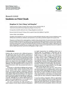
2 Objectives The goal of this work is to create and evaluate a mobile solution to transfer the stream of depth images from a mobile device to a stationary system to allow further processing on a more powerful computer. Even though processing on a mobile device with limited hardware might be possible (see [10]), it is the task of this work to evaluate whether transferring the data to a stationary system is practical and what quality and throughput can be achieved. The mobile device is an Android device having an OpenNI-compatible depth sensor connected, such as the aforementioned “Structure” sensor. In a mixed reality interaction scenario, this android device could be part of a mixed reality interface with a depth sensor attached to it. To preserve the freedom of movement of the user, the transmission shall be over a wireless network. From these requirements, the Samsung Galaxy Tab2 10.1 Wi-Fi has been chosen as a mobile device. Its dual-core processor runs a 1 GHz, which is surpassed by most of the currently available mobile devices. While sometimes referred to as “depth frames” in this work, depth images and depth frames are to be considered the same. Fig. 2.1 roughly sketches the final architecture to be developed in this thesis.

Figure 2.1: A schematic of the mobile device and the stationary system. (a) Structure sensor, (b) typical raw depth image, (c) android device, (d) wireless transmission, (e) stationary system, (f) an artistic depiction of a hand in a point cloud. The hand is shown as a polygon mesh.

4

2 Objectives

To ensure that the speed and accuracy is good enough for gesture recognition and gesture control, different strategies will be developed and used that shall increase the speed and accuracy of the transmission. Two aspects are significant: Firstly, the use of a stationary system that takes over the further processing of the depth images for different consumers to take the computational load off the mobile device, and secondly, the transmission speed. It has to be examined whether compressing depth images or point clouds on mobile devices makes an improvement over the transmission of raw, uncompressed images. Compression algorithms will be tested and compared with the transmission of raw images. The final architecture will cover (a) accessing the depth sensor from a mobile device, (b) receive depth images from the sensor, (c) compressing, (d) transferring, (e) uncompressing and (f) converting them to a point cloud, as shown in Fig. 2.1.

5

3 Related Work Point cloud streaming is not a new topic and was presented in multiple theoretical and practical studies throughout the last 10 years. These works solely refer to the distribution of point clouds from a stationary system with significant computation power to other consumers. A mobile solution for point cloud streaming, especially for Android-based architectures, was unavailable. Furthermore, there were only few solutions to connect a mobile android device with depth sensors. Sec. 3.1 will introduce available solutions for connecting depth sensors on mobile devices. Sec. 3.2 presents architecture variants in the context of point cloud streaming and shows two different approaches, namely point cloud and depth image compression, to solve this task. Sec. 3.3 explains methods for point cloud compression and Sec. 3.4 presents different methods for depth image compression.

3.1 Depth sensors on mobile devices Connecting depth sensors to a stationary computer, processing sensor data and creating point clouds is an easy task. It involves downloading and installing drivers and launching a sample application. Generating a point cloud on a stationary computer and streaming the point cloud to an Android device has also been done before. The point cloud viewer [14] for Android, available as part of the Robot Operating System, receives and loads a single point cloud structure in up to 30 seconds, after which the user can navigate through a virtual world of points. There are two solutions where a depth sensor is connected to a mobile Android device. The aforementioned Project Tango and the Odroid-X [17] has demonstrated that a Kinect sensor can be connected to an Odroid-X device running Android. A demo application uses basic object tracking to move a rectangle on the screen. The solution runs on native code that has never been published by the author.

6

3 Related Work

3.2 Depth image and point cloud streaming Streaming depth information from Android devices to powerful stationary computers, in order to defer complex hand recognition tasks, has not been done by now. As a consequence, there is a need to implement basic methods and algorithms for efficient transmission from mobile Android devices. Most of the publications about depth information streaming have developed or compared compression algorithms that require powerful hardware or cannot run in real-time. These algorithms can be classified into two classes: Point Cloud Compression Point clouds are generated first, which are then transmitted over the network. To achieve sufficient transmission throughput, several point cloud compression algorithms have been developed. Sec. 3.3 will discuss recent solutions for point cloud compression. Depth Image Compression Depth images are streamed over the network, and then converted to point clouds. The main task on the mobile device will then be to efficiently compress depth images. Sec. 3.4 will introduce several methods and applications for depth image compression.

3.3 Point Cloud Compression Solutions for compressing point clouds have been developed, using predictions, temporal and/or spatial optimizations [6] [11], octrees [31] [13], wave functions [4], dynamic generation of surface normal functions [18] and few of them were directly committed into the PCL source tree [29]. To convert depth sensor images to point clouds, the built-in CoordinateConverter from OpenNI can be used. However, the OpenNI documentation recommends to delay the calculation of point clouds as long as possible since it is an expensive operation. Additional algorithms should determine the regions of interest prior to conversion [21]. Therefore, these compression methods are introduced briefly, but not taken into consideration in the course of this work.

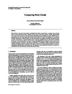
3.3.1 Adaptive arithmetic coding for point cloud compression In the publication of Daribo [6], point clouds are compressed and encoded as 3-D space curves. In point clouds that have been captured using structured light cameras, individual point locations are predicted by exploiting the homogeneity of surfaces. The proposed framework uses a 3-D extension of the Freeman chain code to encode 3-D space curves describing surfaces.

7

3 Related Work

The curve is a chain of points, which enclose sections of the curve with a turning angle near zero, and with a possibility to exploit repetitive patterns and similarities. Adaptive arithmetic coding is then used to compress floating point values losslessly. It requires less bits to store floating point values in frequently used intervals than those in rarely used intervals. The peak signal to noise ratio (PSNR) for sample images was evaluated for data stored with 16 to 28 bits per point. The author did not do any time performance measurements.

Figure 3.1: Sampled point cloud partitioned into series of curves with respect to the projected grid pattern. Curves are discriminate by different colors. [6]

Figure 3.2: 2D example of plane curve sampled at intervals of arc length ∆S. Each point has a turning angle α as the angle between two consecutive segments. [6]

3.3.2 Predictive Point-cloud Compression Predictive Point-cloud Compression [11] omits the construction of meshes and geometric models and instead puts all the points into a spatially sequential order. Points are then predicted from previously coded neighbors with simple prediction rules such that only corrective vectors need to be encoded. To create a spatial sequence in the data, a spanning tree is used. Points are encoded in the spanning tree and corrective vectors are added. Entropy coding and arithmetic

8

3 Related Work

coding is used to further compress the data. The author measured that a 2GHz PC requires 20 seconds to encode 100.000 points.

Figure 3.3: prediction trees built with linear prediction (bunny is a 3d scan). [11]

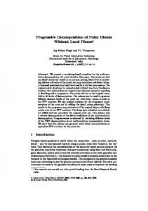
3.3.3 Octree-based Point-cloud Compression Schnabel [31] uses an octree and encodes the points’ locations as its containing cells’ centers. Octrees divide a bounding box into equally-sized partitions, two for each dimension. To encode each node of the octree, a single byte stores whether each child node is occupied. In this work, the occupied child cell configurations and the number of empty cells are predicted, using planes and single child cells. To encode color information into the point cloud, a mean color index is encoded for each octree level and then predicted for their children. The performance of this scheme allows encoding point clouds with 2 to 8 bits per point.

Figure 3.4: A cell is to be subdivided. Those child cells that are closest to the surface approximation FQC are more likely to be occupied. [31]

3.4 Depth Image Compression The raw stream of depth images is a series of uncompressed 16-bit grayscale images, where each pixel is the distance from the sensor, measured in millimeters. A 16-bit number can handle values up to 65535, which is, in theory, the maximum distance in millimeters that can be represented in this format. Depending on the sensor and the requested stream, the resolution

9

3 Related Work

of these images is either VGA (640 x 480 pixels), QVGA (320 x 240 pixels) or even smaller. The data structure is exactly the same as the depth data from the RGB-D sensor described by Coatsworth [5]. The most widely known image compression format is JPEG. It is known for its great performance shrinking average photos by 33% up to 90% in size without noticeable artifacts. JPEG uses a color space transformation that converts pixels made of red, green and blue values (RGB) to a brightness and two color shift values (YUV). Using this transformation allows to receive better compression quality, especially by downsampling the color shift channels more than the brightness channel. High frequency brightness changes which a human eye might hardly see are removed after a discrete cosine transformation and quantization. Movie compression algorithms such as H.264 or VP8 can go beyond that, as they take full advantage of areas in the image that changed only slightly from two consecutive frames. However, most of the image and movie compression algorithms fail to encode more than 8 bits per color channel. Our source image has 16 bits of depth in one single color channel, and the majority of the few file formats capable of storing images with higher dynamic range apply almost no compression to them. Some simple image compression algorithms use surrounding pixels and use linear prediction to reduce the entropy required to encode the pixel values. Data compression formats such as Deflate recognize patterns in the source data and also reduce the entropy required to encode them. Works and algorithms that solve this problem can be subdivided into two categories. Sec. 3.4.1 will present a method to encode 16-bit streams using lossy 8-bit color compression formats. Sec. 3.4.2 will present methods that encode 16-bit frames natively.

3.4.1 Three channel 8-bit encoding Pece [26] compresses depth videos using unmodified standard video encoders with three color channels of 8 bits each. In the cited work, the results after encoding and decoding with different bitrates and three different compression algorithms (JPEG, VP8 and H.264) are compared. To convert the 16-bit grayscale image into three 8-bit color channels, a pre-processing step is made before the results are fed to the encoder. Similarly, after decoding the compressed stream, a post-processing step decodes the original depth value from these three color values (see Fig. 3.5).

10

3 Related Work

Figure 3.5: Graphical overview of the proposed method. The original 16-bit depth map is encoded in an 8-bit, three-channel image and is then processed by a video encoder and transferred over the network. When received, the three-channel image is decoded through the video decoder and is then processed by our method to reconstruct the original 16-bit depth map. [26] Using movie encoders can be advantageous when depth and color information are encoded at the same time, because using the same encoder for both types of information will make the encoding and transmission less complex. The aforementioned image and movie encoders use quantization and downsampling to achieve high compression levels. Such methods strongly affect sharp corners or high-frequency changes in data, so the pre-processing and post-processing should not add continuity gaps or carryover jumps into the source image. The work suggests that one robust color channel contains the most significant 8 bits of the depth image, while the other two color channels encode the least significant bits. To ensure continuity, the actual depth values are transformed using two linear triangle wave functions (see Fig. 3.6), one for each remaining color channel, differing in their frequency.

Figure 3.6: L (blue), Ha (green) and Hb (red) with w = 216 . For illustration, np = 2048 is set unusually large, and the ordinate shows integer values rather than [0,1]-normalized values. [26]

11

3 Related Work

If the encoder uses color space transitions from RGB to YUV before starting the frame encoding, the source image is fed to these three color channels directly instead, to increase the accuracy of the data transferred. The Y-channel, which stores the brightness value of each pixel, typically has a higher precision and stores the most significant bits. The U and V channel, used for the tone value, have a lower precision and are used to store the triangle waves. In the conclusion, test results were shown, and a 3 GHz quad-core processor requires 8 milliseconds for each QVGA frame and 30 ms for each VGA frame to encode. The author makes no assumptions about the performance on mobile devices, but it can be assumed that, unless hardware optimizations for the encoder are in use, these durations can be much longer on a mobile device.

3.4.2 Frame-by-frame encoding Frame-by-frame encoding means that each frame is individually compressed and transferred one by one. The advantage is, that any single frame can be dropped from the queue without interfering with other frames. Also, unlike movie encoding, no references are made to frames in the future, which decreases the latency in both the encoding and the decoding process. Dropping frames is also very useful when any of the components in the chain (mobile device, network bandwidth) can’t keep up with the amount of data. Generic compression algorithms Coatsworth [5] describes a UAV mounted with a RGB-D camera, that encodes the color image using JPEG, and the depth image using lossless compression algorithms. Both encoded results are transmitted over a wireless network and then decoded on the receiver (cf. Fig. 3.7). The author compared three different available lossless compression algorithms for the depth images: bzip2, zlib and snappy.

12

3 Related Work

Figure 3.7: System diagram of server-client system and compression steps [5] With different slow test platforms used for encoding and transmission, different average frame rates were achieved. The paper concludes that zlib, being the average of the three algorithms in terms of speed and compression rate outperformed the other algorithms on better hardware, while snappy can achieve better frame rates when inferior hardware was used. Although not mentioned in the cited work, the deflate compression, which is a combination of Lempel-Ziv 77 and Huffman coding, may achieve similar results. It is already integrated into the JRE (Java Runtime Environment) and therefore quite portable. The slow compression speed of BZip2 will most likely not be worth the slightly better compression ratio. To use the BZip2 compression in Java, the jbzip2 compression/decompression library [9] can be used or the Apache CBZip2InputStream / CBZip2OutputStream classes. The first library is a pure Java implementation, and thus more portable than the Apache classes, which rely on native libraries. The Author furthermore claims that jbzip2 is typically 5% to 10% faster than the native implementation. For the Snappy compression algorithm, there is an implementation inside the Hadoop IO Compression library, which is part of the common library package of the Apache Hadoop framework. It uses a lot of native code and has dependencies to environment-specific memory management hacks which abuse exposed methods in earlier versions of the Java Runtime Environment. Another implementation of the Snappy algorithm [34], written in pure Java also uses the UnsafeMemory functionality and inherits classes from the Hadoop framework, but the use of UnsafeMemory can be easily stripped by removing a few files from the source.

13

3 Related Work Jpeg-LS Jpeg-LS, not to be confused with “JPEG Lossless” is a lossless image compression format capable of compressing 16 bits per channel images. It uses a predictor and context modeler for gradients and run length encoding for flat regions (see Fig. 3.8). It is based on the LOCO-I algorithm developed at Hewlett-Packard Laboratories, and a thorough description of this format has been made [27]. Performance measurements have been performed with software and hardware implementations [30].

Figure 3.8: A casual template and a basic block diagram for Jpeg-LS. [27] CharLS [7] is a library that compresses images using Jpeg-LS lossless compression format. It supports up to 16 bit per color channel and also grayscale images. In comparison to JPEG 2000 it is claimed to be about 3 times faster. The CharLS library offers 6 customizable constants, namely allowedLossyError, MAXVAL, T1, T2, T3 and RESET. Experiments, where these values are changed have shown that the compression ratio can be improved by carefully selecting these values [27]. In this library, changing allowedLossyError to a non-zero value has an unexpected result that will be discussed in Sec. 6.3. BPG BPG is a lossy image compression format [1], and is based on the Intra-Frame encoding of the HEVC (High Efficiency Video Coding) video compression standard, also known as H.265, and capable of compressing 14 bits per channel images. As 14 bits equal 16384, and depth pixels are measured in millimeters, the maximum distance is reduced from over 65 meters down to little more than 16 meters, which is more than needed for hand gesture recognition. However, the special 0.1mm mode of the Structure sensor, which increases the maximum accuracy for

14

3 Related Work

near objects to 0.5mm, reduces the maximum distance to 6.5 meters at 16 bits and 1.6 meters at 14 bits, which will constrain the ability to scan the surrounding environment. BPG is also dependent on many libraries, namely the x265 library and the JCTVC reference encoder, which makes it difficult to compile with unusual build environments. Only if the JCTVC encoder is used, BPG can use bit depths higher than 8 bits per channel. The JCTVC reference encoder is even more difficult to compile, as it has many dependencies to other libraries. The build script obtainable from the BPG developer uses path rewrites, which are neither supported by the Android NDK toolchain nor by the gradle scripts. PNG and TIFF The PNG and TIFF formats also allow encoding images with 16 bits per color channel. The compression rate of PNG is very low in this case, and almost no compression is noticeable when the TIFF format is used. The ImageIO classes from Java support 16-bit PNG images if the user happens to have the Java Advanced Imaging API installed on his computer. This API only exists for 32-bit Windows and a couple of other operating systems and is closed-source, so it won’t work on many newer systems. Its native code was created at times when Java was still developed by Sun Microsystems, Windows ran on a 32-bit architecture and Android was not known as an operating system at all.

3.5 Conclusion It has been shown that Android-based software for streaming depth information from depth sensors are currently not available. Although works and methods exist for point cloud compression, currently there is no method suitable for mobile devices. OpenNI developers have recommended to delay the calculation of point clouds as long as possible. For the scope of this work, using a two-stage architecture for the distribution of point cloud data acquired from a depth sensor connected to an Android device is the most promising: Depth images are streamed over the network to a stationary device, and then redistributed as a point cloud. The point cloud generation will thus be performed on a powerful computer, and the efficiency of the depth image streaming is focused on in the course of this work. From the algorithms introduced, the following will be examined in this work: Jpeg-LS, Deflate, BZip2 and Snappy. PNG support can be used on systems running on a 32-bit Windows environment. The Deflate, Bz2 and snappy compression algorithms can run in pure Java and for Jpeg-LS and BPG, a C library is available. Due to the unsatisfiable requirements of the build environment, BPG is passed on in this work.

15

4 Requirements Analysis In Sec. 2, two major subsystems with roles have been introduced: The mobile Android device and the stationary system. Based on a preliminary decision, different requirements for the different subsystems are as follows. They are divided into functional requirements for mobile and stationary systems respectively, and non-functional requirements. If the scope of a requirement is not further specified, it applies to both systems.

4.1 Functional requirements • The mobile application has to establish a connection to the depth sensor. • To reduce the required bandwidth on the wireless transmission, the system should be able to compress depth frames using different algorithms. • To compare the quality of the compression algorithms and the uncompressed transmission among each other, the system shall show the speed of the transmission and the required bandwidth. • To get a good estimation for the cost of depth image pre-processing, a depth image viewer similar to the NIViewer from earlier OpenNI packages should be developed.

4.2 Non-functional requirements Configuration: Configuration settings such as IP addresses, sensor parameters and compression mode should be easy to change. At runtime, the application shall choose the desired quality when acquiring depth frames from the sensor. Maintainability: The system shall have low complexity. By having the exact same architecture both on the stationary system and on the Android device can reduce the complexity of the system and thereby improve the maintainability. For example, both systems acquire information, compress or decompress it and then transfer, visualize or process it directly.

16

4 Requirements Analysis Openness: Choosing an open architecture is preferred, as this will allow the architecture to be used as an extension to existing frameworks, e.g. a gesture recognition software. Extending to an existing architecture requires an open architecture in order to access data streams by the recognition algorithms, by means of open interfaces. Performance: A low latency, a high resolution and a high frame rate is desirable, as all of this improves the quality of the data required by the recognition algorithms. A low latency will help responding to and reacting on gestures sooner. Reporting: Transmission speed, such as the average bandwidth and frame rate shall be displayed on both devices. Automatic measurements shall be performed to determine the achieved frame rate, compression ratio and bandwidth usage. Latency however will be extremely hard to measure, because independent systems will have different clocks. A separate physical device, like a stopwatch, is required to perform the latency measurement.

17

5 Design and Implementation This section introduces the system design and facilitates the implementation by a thorough specification. As has been pointed out in Sec. 2, the architecture has (at least) two independent systems that are connected over a wireless network. Sec. 5.1 details the system architecture already introduced in Sec. 2. Sec. 5.2 provides the ways, how each system’s configuration can be set up by the user. Sec. 5.3 continues with the architectural patterns used in this software architecture, namely the Source-sink concept, the Strategy pattern and the Factory pattern. Class diagrams, interfaces and characteristics of each implementation are specified in Sec. 5.5. Sec. 5.6 describes necessary changes to the development environment and the OpenNI2 framework to allow accessing the Structure sensor from an Android device. Finally, Sec. 5.7 reviews this section.

5.1 System Architecture To describe the system architecture, the hardware schematic sketch is shown again in Fig. 5.1 to logically illustrate the whole chain from the depth sensor to the interface for detection algorithms. Two separate systems, one being the mobile device and one being the stationary system, are processing the depth data.

18

5 Design and Implementation

Figure 5.1: A schematic of the mobile device and the stationary system. (a) Structure sensor, (b) typical raw depth image, (c) android device, (d) wireless transmission, (e) stationary system, (f) an artistic depiction of a hand in a point cloud. The hand is shown as a polygon mesh. The mobile device is in charge of accessing the depth sensor and acquiring individual depth frames. It compresses them, depending on the configuration, and transfers them over a wireless network. To interact with the depth sensor, the OpenNI2 framework will be used. To compress the depth data, compression algorithms will be included and used. To transfer the data, another module is required that delivers the frames to a stationary system. For the sake of reliably, a TCP connection is chosen over UDP, because the frame sizes are assumed to be larger than the maximum transmission unit of most network connections, and using TCP is assumed to be less complex than reinventing the wheel using a custom streaming implementation. A network operator may automatically assign IP addresses to all connected devices which makes it necessary to configure the systems to allow finding each other on a network. Thus, the last module required is a graphical interface for user interaction, which is detailed in the following section. All these modules will be packaged together into an Android application. The stationary system is in charge of receiving the depth frames from the network. It decompresses them and offers them to consumers for further processing. To receive the frames, a module is required that establishes a TCP connection with the mobile device and receive the compressed frame data. To decompress the data, the same compression algorithm is needed that has been used for compression. To allow further processing, an interface is required that recognition algorithms can use. A helpful addition is a window that serves as a visual feedback for the transferred data, which is detailed in one of the following sections. All these modules will be packaged together into a single software.

19


5.2 Configurability of the whole system Each of the system has to be individually configured, to take on the correct role in the chain. The configuration will cover what is used by each system to acquire depth data, how it is processed and where it goes after it has been processed. This also includes hostnames, network ports, sensor parameters such as the resolution and field of view, frame and stream information. In an Android system, the PreferenceActivity allows for much of the required functionality. It has number, text, checkboxes and drop down selections, which are suitable for e.g. screen resolution, hostnames, enabling or disabling features and selecting out of a list of available algorithms. Fig. 5.2 is an example of a PreferenceActivity to change settings before starting the transmission by a mobile device.

Source Config

Codec Config Sink Config

Data Config

Frame width:

640 pixels

Frame height:

480 pixels

Sensor type:

Depth sensor

Sensor mode:

1mm resolution

100µm resolution

Sensor fps:

30fps

Activate

Your IP address: 192.168.0.1

Figure 5.2: A mockup of the PreferenceActivity that will be used to change settings on an Android device. On a stationary system however, many more possible solutions exist that avoid recompiling the program from source code. A configuration file can be edited much more easily on a stationary system than on a mobile device. Parameters can also be given on startup or using a startup script. A configuration window, much like the PreferenceActivity on Android can be used. This work focuses on the open architecture concept, that when actually feeding a real handtracking algorithm to the streaming architecture, a lightweight loader may provide different configurations on the fly. It is sufficient to include a simple loader that provides a configuration for testing purposes, and replace it with a different loader when including it in a hand-tracking solution.

20


5.3 Architectural patterns Architectural patterns have proven themselves as guidelines for a good system design. To satisfy the non-functional requirements from Sec. 4.2, three commonly used design patterns, namely the Source-sink concept, the Strategy pattern and the Factory pattern are used in this software architecture. In the following, each of them will be introduced in more detail.

5.3.1 Source-sink concept The source-sink concept shown in Fig. 5.3 is frequently used during the encoding or decoding of video streams. In such context, the source is a provider of information (a camera, a network stream or a recorded file), the sink is a receiver of information (a television, a network uplink or recording into a file) and a filter usually applies transformations (change resolution, change color space, compress or decompress).

Source

Codec

Sink

Figure 5.3: The source-sink concept. The data comes from the “source”, is transformed in the “codec” and ultimately sent to the “sink”. Here, the source is “something that obtains an image”, the codec, a special filter with the transformations ’encode’ and ’decode’ is “something that reads the image and creates a modified version, and the sink is “something that delivers an image”. This concept proves useful for two reasons: 1. By enforcing clear, slim interfaces, especially for the data transfer, any of the three components can be substituted without any needs to handle extra interoperability cases in the other components. As a consequence, the handling of optional information and metadata such as frame id and sensor parameters must be realized by other functionality (see Sec. 5.2). 2. By using an abstract pattern, the implementation of every component can be adjusted depending on the designated runtime environment. As Fig. 5.4 demonstrates, choosing different implementations for modules that obtain images, both systems, the mobile and the stationary system, can be configured using the same

21


architecture and concepts. To ease development, it is feasible to also include modules that replace complex processes with simpler ones that don’t fit the whole scenario. As an example, an access component for the depth sensor can be replaced by a component that does nothing else than returning a static, procedurally generated test image over and over.

Source

Codec

Sink

Mobile device:

Depth Sensor

Raw

CharLS (encode)

Compressed data

TCP Server

Compressed data

CharLS (decode)

Raw

Window

Stationary system:

TCP Client

Figure 5.4: An example implementation of the source-sink concept with specific components. An Android device is compressing images, a stationary system is decompressing images, using the same workflow.

5.3.2 Strategy pattern The strategy pattern defines a family of substitutable algorithms that implement the same interface. It also eliminates control structures in the main program and uses the application context in order to select the right implementation. By applying this pattern to the source-sink concept, the main program only works with the interface and the implementations can be easily substituted. The actual algorithms behind them, including initialization and configuration are hidden inside multiple implementations that can be chosen from.

5.3.3 Factory pattern The factory pattern is used to retrieve the required implementation of an algorithm dynamically at runtime. A set of concrete factories are available to instantiate the required classes on demand. They can also abstract the way components need to be configured. Different runtime environments can have different sets of factories to choose from. Fig. 5.5 shows a typical application of the strategy and the factory pattern using the CharLS codec as an example implementation.

22


This solution would increase the class count significantly and make the code less maintainable. Therefore, this work uses a modified variation of the factory pattern: • The factory is changed from an interface to an abstract class with the two static methods getFactory(String) and addFactory. • All available factories are constructed and added using the new static methods at start of the program. • Factories available on a specific platform are implemented as anonymous inner classes in static code. With this modification, factories are identified and selected by a simple String value in the configuration.

Main Main(Config)

CodecFactory

Codec

+getCodec(Config) : Codec

+encode(ByteBuffer, ByteBuffer, int) : int +decode(ByteBuffer, int, ByteBuffer, int)

CharLSCodec

CharLSCodecFactory


+getCodec(Config) : Codec

Figure 5.5: The method getCodec on the CodecFactory interface returns objects of type Codec. What implementation of Codec is returned depends on which implementation of CodecFactory is handling the method call.

5.4 Program flow The simplest program flow that successfully encodes (or decodes) a stream of depth frames is shown in Fig. 5.6. After initializing the source and sink, it enters an endless loop to retrieve,

23


encode and deliver one frame after another. While it serves well as a first prototype, it needs to be modified significantly to take advantage of pipeline parallelization by means of multithreading.

Program flow Initialization

Initialize sink

Processing

Initialize source

Fetch image from source

Encode / Decode

Deliver image to sink

Figure 5.6: The program flow separated into five steps. Note the repetition after the last step.

5.4.1 Multi-threading Multi-threading has an advantage of increasing the throughput and thus the frame rate limit a compression algorithm may enforce, by encoding several frames at the same time. However, this can also increase the average processing time for each single frame and thus the latency. The more worker threads in use, the more frames can simultaneously stay in the encoding or decoding chain before a new frame is read from the sensor, under the assumption that the worker threads run much slower than the time it takes until a new frame is acquired. The number of worker threads should thus be configurable. In a thread pool pattern, every thread can request the next task from the task queue, process it and request the next task from the queue (see Fig. 5.7). Task Queue ...

ThreadPool

Completed Tasks ...

Figure 5.7: A sample thread pool (green boxes) with waiting tasks (blue) and completed tasks (yellow).

24


The thread pool pattern is very favorable, but its conventional implementation has a lot of drawbacks. To use this concept for time-critical processing of a large bulk of data, modifications have to be made: Fixed number of threads Typical thread pools can add and remove worker threads dynamically on demand. Here, the amount of threads is fixed to prevent creating and destroying resources unnecessarily. Task objects and queues Typical thread pools work with a queue of unfinished task objects. This would mean that frames are automatically pulled from the sensor and task objects are put into the task queue containing the frames in memory buffers. This is disadvantageous because it increases the latency with every single frame waiting in the queue. Also, a task object would cause typical overheads of creating and throwing away objects and memory buffers. The solution to this is not having any task objects and queues at all. Each thread gets assigned independent resources and memory buffers and recycles them after each completed “task”. Instead of task objects, the threads access the source directly to acquire a new depth frame. The task as such exists only as a frame inside the memory buffer. After finishing the processing, the threads deliver the processed frames to the sink and obtains the next frame. Keeping frame order The solution must ensure that the frame order won’t be changed. Processed frames should be delivered to the sink in the same order they were obtained from the source. The order in which the threads access the sensor is predictable. To ensure that the worker threads don’t fight over the next available depth frame, they will take turns at accessing the depth sensor. The threads will also have to wait until they can deliver processed frames to the sink and synchronization becomes necessary. By knowing the order in which threads access the source and requesting their delivery in the same order, it won’t be changed. Synchronization A scheduler determines when a thread may be allowed to read the depth frame. It gets notified by the worker thread that the read has completed and lets the next thread access the depth

25


sensor. The threads are also scheduled in a predictable order, to allow sorting the processed frames without looking up frame IDs in a list. After a worker thread has read an image from the depth sensor, the compression algorithm is starting its work, after which the thread pauses until the processed frame may be delivered. A delivery thread knows the predictable order in which the processed frames have to be received from the threads and arranges them in the correct order. The delivery thread notifies the sink that a new frame has been processed. Only after the sink has finished accessing the result, the worker thread may start from the beginning, otherwise the memory area may be overwritten with the next frame data while the sink is reading it. The advantage of this restriction is that both the source and the sink can reference the same memory mapped area designated for a worker thread and do not need to copy the binary data at all. Java uses synchronized objects to acquire locks and concurrency utilities to accomplish the aforementioned constraints. To run the thread pool, the scheduler, the delivery chain and the worker threads are initialized and started. The new program flow is outlined in Fig. 5.8. The number of synchronization points is higher than in conventional thread pools that potentially shuffle the frame order. The five synchronization points are: • The scheduler waits for the next worker to become ready • The worker waits for the scheduler to send a start signal • The scheduler waits for the worker to obtain a frame • The delivery waits for the worker to complete processing • The worker waits for the delivery to complete the delivery

26


Scheduler

Worker Thread

Delivery

A worker wants to retrieve the next image

The left chain supplies a new image to the worker

The follow-up image for the sink is ready

Supply a source image to the worker thread

Compress the image, if requested (configuration)

Supply the image to the sink

Decompress the image, if requested (configuration)

The image has been retrieved

The image is ready. Wait for clearance from the right chain

The sink has finished reading

Remember the image counter and wait for the next worker

Notify the left chain that a new image can be supplied

Allow the worker to retrieve the next image

Figure 5.8: The scheduler and delivery thread synchronize the worker’s access to the source and sink. The upper hexagon of the worker thread causes an iteration of the scheduler, and the lower hexagon causes an iteration of the delivery.

5.5 Class diagram The design consists of 5 classes controlling and coordinating the whole process and parallelization. The factory pattern requires two classes for each factory, and another two classes for each implementation. Counting all of them, their helper classes and a few other exceptions, 39 classes are required on Android and 48 classes for the stationary system as it has access to more encoders. The Android user interfaces uses 5 classes for the setup, while the stationary

27


system needs only a single one. That being said, the stationary system appears to be slightly more complex having 54 classes in total compared to the 49 classes on Android. Thus, three major parts of the solution are visualized in each of the class diagrams. Sec. 5.5.1 describes all interfaces needed by the main class during the processing. Sec. 5.5.2 includes every factory and implementation, which are used by the main class during the initialization. Sec. 5.5.3 outlines the additional classes needed on an Android device. Finally, the NIViewer is described in Sec. 5.5.4.

5.5.1 Main routine and parallelization Fig. 5.9 contains all the classes needed by the Main routine, except the factories used to initialize the source, codec and sink, which follow in Sec. 5.5.2.

Config +String source, compression, sink +boolean compress, decompress +String sourceUrl, sinkUrl +int sourcePort, sinkPort, threads +short x, y +byte depth, mode, fps +int frameId +float fovX, fovY +boolean sinkControlled, benchmark +boolean debug, condition

Scheduler : Thread

Source +readImage(Config, ByteBuffer) : boolean

Main -Config config -Source source -Codec codec -Sink sink -ArrayList -Thread schedulerThread -Thread deliveryThread +Main(Config config)

CompressionWorker : Thread -ByteBuffer sourceBuffer -ByteBuffer compressedBuffer -boolean canStart -boolean obtained -boolean complete -boolean canReset -Object startLock -Object obtainLock -Object completeLock -Object resetLock +reset()

Delivery : Thread

Sink +initialize(Config) +writeImage(Config, ByteBuffer, int) : boolean

Codec +encode(ByteBuffer, ByteBuffer, int) : int +decode(ByteBuffer, int, ByteBuffer, int)

Figure 5.9: A class diagram that contains the classes responsible for the Main routine and parallelization.

28

5 Design and Implementation Config This class contains all the settings required to change the sensor parameters, network addresses or compression algorithms (cf. Sec. 5.2). Some fields can be changed during runtime by the source and sink (e.g. fov, the field of view, which is required to calculate point clouds, and the frameId, which is necessary to be updated independent to the return values of readImage). The flag sinkControlled will also change the initialization order; if enabled and TCP is used as a sink, the TCP server (a concrete implementation of sink) retrieves the desired resolution and other parameters from the first connecting client before the source is initialized. Finally, the condition flag helps the CompressionWorker understand why no new depth frame can be obtained. If vital components fail, or the user wants to stop the processing, the flag is changed to let the workers interrupt naturally. Main The Main class has a Main method that initializes all the threads mentioned in Sec. 5.4. It holds copies of all the other classes shown in the diagram, and because the Threads are inner member classes, they can access them as desired. Scheduler, CompressionWorker, Delivery Scheduler and Delivery change status flags and locks on the CompressionWorker, and CompressionWorker only needs the references to the interface implementations of the source, codec and sink, and the Config instance. The detailed program flow of these threads has already been explained in Sec. 5.4.

5.5.2 Source-sink concept and its factories The class diagram in Fig. 5.10 shows the factories and their interfaces, and how they are used by the Main routine. The following subsections will detail the behavior of these classes and describe concrete implementations of each interface. The factory pattern is outlined in Sec. 5.3.3. Exceptions and extensions of them are described in the following subsections. Each abstract factory contains static code that instantiates all the available factories, and adds them to a list with a call of addFactory. A certain factory implementation can be obtained by calling getFactory(String). External libraries can add their own factory implementations to extend the available sources, codecs and sinks in this application, without needing to change any of the original source code.

29


Hereinafter, the factories and interfaces are described (blue boxes in the diagram), and their respective implementations contained in this solution for different source, codec and sink types (green annotations in the diagram).

Main Main(Config)

SourceFactory

CodecFactory

+getFactory(String) : SourceFactory +addFactory(SourceFactory) +getName() : string +startSource(Config) +stopSource(Config) +getSource() : Source

SinkFactory

+getFactory(String) : CodecFactory +addFactory(CodecFactory) +getName() : String +getCodec(Config) : Codec

+getFactory(String) : SinkFactory +addFactory(SinkFactory) +getName() : String +getSink(Config) : Sink

Initializing sources is complex. FactoryImpl sets up all parameters from Config for SoC. FactoryImpl acts as a responsible controller

Source

Codec

Sink

+readImage(Config, ByteBuffer) : boolean

Implementations: Test image (TestSource) RAW image (RawFileSource) PNG16 image (PngFileSource) ONI record (OniFileSource) ONI stream (OniStreamSource) TCP stream (TCPSource)

Examples written in italic only work on Win32, Linux32 or Linux64 systems


Implementations: Clone (ByteCloneCodec) Copy (ByteCopyCodec) Bz2 (Bz2Codec) CharLS (CharLSCodec) Deflate (DeflateCodec) JpegLS (JpegLSCodec) PNG (PNGCodec) Snappy (SnappyCodec)

+initialize(Config) +condition(Config) : Boolean +writeImage(Config, ByteBuffer, int) : boolean

Implementations: TCP stream (TCPSink) Window (WindowSink) Point Cloud (WorldCalculatorSink) Clone & Copy are for debugging purposes. Window only works on desktop Java with AWT support.

Figure 5.10: A class diagram that focuses on the factories and the various implementations of the source-sink concept. SourceFactory Each SourceFactory implementation is responsible for initializing and finalizing the resources of its respective Source implementation. This practice allows the factories to read the Config class and translate the initialization parameters to those needed by the sources. Some sources are more complex to initialize than others. The OniStreamSource requires access to the depth sensor, and a reference to the current activity is needed on Android platforms (see Sec. 5.5.3). Obtaining this reference has to be done in the factory. If the TestSource is used, which creates a procedurally generated test image, it doesn’t need any initialization.

30

5 Design and Implementation Source Source offers the method readImage that inserts new data into the ByteBuffer. Additionally, it may update fields on the Config, such as the frameId. It can also change the condition flag to gracefully shut down the application if the pipe to the device or remote system is broken. The solution contains implementations for different source types, if they are available for the designated environment. They are described in the following: TestSource The TestSource generates images procedurally, as shown in Fig. 5.11. The gradients are useful to test the brightness clipping feature for the AWT window: if the white cut-off value is set low enough, the black horizontal lines turn into gradients. It is the first source to be implemented to test how Java code works with ByteBuffers.

Figure 5.11: The 16-bit grayscale test image contains randomly colored squares and three different gradients. The black horizontal lines are incrementing the intensity one unit per pixel, which can hardly be seen on regular screens. RawFileSource The RawFileSource accesses a file in the local file system and reads it into the ByteBuffer. As an uncompressed depth frame is a 16-bit grayscale image, the file must have twice as many bytes as it has pixels.

31

5 Design and Implementation PngFileSource The PngFileSource also accesses a file in the local file system, but calls the ImageIO classes from Java and then accesses its raster to acquire the raw image. In this context, a 16-bit grayscale PNG is the easiest file type to deal with, if the user happens to have the Java Advanced Imaging API installed on his computer. Consult Sec. 3.4.2: PNG and TIFF for more details about the JAI API. OniFileSource and OniStreamSource The OniFileSource initializes the OpenNI2 library using a local file path as the sensor device. This plays back a previously recorded OpenNI2 file. The default setting is to not skip any frames and repeat the sequence after the end of the recording has been reached. The OniStreamSource also initializes the OpenNI2 library, but chooses a connected sensor instead. After the initialization, the desired stream type is chosen and physical parameters of the sensor such as the field of view is stored in the Config class. Reading an image from the OpenNI2 library is followed by an immediate release of the memory mapped framebuffer, to prevent leaking memory over time. TCPSource The TCPSource creates a TCP client using the SocketChannel from Java’s NIO library. Choosing this over more usual classes for TCP connections has an important advantage, when reading and writing data from and to memory-mapped buffers. It is harder to interleave different types of data structures, so this implementation reads a 8-byte header first and then reads the exact amount of bytes specified in the header packet. The frame size and frame Id exactly occupy these 8 bytes, so to transfer other information such as the sensor parameters required for the point cloud generation, a special condition distinguishes this from an extended header type consisting of three stacked headers. The implementation does not need to be thread safe (i.e. protect the header from being overwritten by another parallel call), because only one thread is allowed to access the source at any time. On initialization, TCPSource also sends configuration parameters to the remote server. If the server reads them, it may change some settings such as the desired resolution. If both systems have different resolutions configured and the TCP server has the flag sinkCon-

32

5 Design and Implementation trolled set in its Config (see Sec. 5.5.1: Config), its configuration gets overwritten before any memory buffer is initialized to a potentially undesirable size. Fig. 5.12 plots the three types of data being transferred.

Typical frame

Sensor parameters

int frameSize

int frameId

int 0

short x

short y

Request header

1 depth fps mode

short x

short y

float fov_x float fov_y Raw frame data fps mode depth pad

int padding

Figure 5.12: Each row in a stack equals 4 bytes. The first two stacks are the communication from the server to the TCPClient, the third stack is the communication in reverse direction. CodecFactory The CodecFactory uses information about the resolution from the Config class, to configure the constructed codecs if necessary. Codec The codec supplies two methods, encode( ByteBuffer compressedData, ByteBuffer uncompressedData, int uncompressedLength) and decode( ByteBuffer uncompressedData, int uncompressedLength, ByteBuffer compressedData, int compressedLength). The compressedLength may never exceed the uncompressedLength, because every ByteBuffer always has the size of an uncompressed image. Some codecs actually need to know the dimensions of the image to initialize additional memory buffers or to set up encoding parameters or metadata. Thus, a subset of codecs inherit a constructor from AbstractCodec to set up the width and height. The solution contains implementations for different codec types, if they are available for the designated environment. They are described in the following:

33

5 Design and Implementation ByteCloneCodec and ByteCopyCodec These two codecs copy the data from a source buffer into a compressed buffer using two different ways. If the buffers are not both initialized as MappedByteBuffers, ByteCloneCodec will fail, indicating that other codecs are also likely to fail, while ByteCopyCodec will not. They are used for debugging purposes. PNGCodec PNGCodec internally works by creating a BufferedImage, updating its raster and encoding them using the same libraries as in Sec. 5.5.2: PngFileSource. Decoding uses the same steps as opening and reading a PNG file. ImageIO is designed to work with binary input and output streams for files on a local file system. To allow ImageIO use the ByteBuffer as a data source for compressed data, two additional classes, the ByteBufferBackedInputStream and ByteBufferBackedOutputStream are used. Although this solution might be less efficient than a direct access, as it actually copies chunks of the memory area into the Java heap, it was better than adopting a two-pronged strategy using different types of the ByteBuffer for special codecs. The availability of PNGCodec is limited to the same conditions mentioned in Sec. 5.5.2: PngFileSource. JpegLSCodec JpegLSCodec also works with the same libraries mentioned in Sec. 5.5.2: PngFileSource. Its internal logic is only slightly different to the PNGCodec. In order to write the compressed data into a stream, a custom ImageWriter or ImageReader is used from the CLibJPEGImageWriterSpi or CLibJPEGImageReaderSpi obtained by the native extensions of Java ImageIO, which is also only available under the conditions mentioned in Sec. 5.5.2: PngFileSource. Bz2Codec and DeflateCodec These two classes implement the Deflate and the BZip2 compression algorithms mentioned in Sec. 3.4.2, using implementations of the InputStream and OutputStream. The InflaterInputStream and InflaterOutputStream used for the DeflateCodec are part of the Java Runtime Environment. The BZip2 implementation uses the JBzip2 library hosted on Google Code. Both compression algorithms allow compression levels to be set. To ease working with these codecs, DeflateCodec has three factories, initializing the codec with the compression

34

5 Design and Implementation levels 2, 5 and 9, and Bz2Codec has two factories for the compression levels 1 and 9. Using very low levels for Deflate such as 0 or 1 is not recommended, because the compressed frame size might be larger than the uncompressed frame size, which results in a runtime exception. CharLSCodec The CharLSCodec class is surprisingly simple: It loads the libCharLS native extension, defines a native interface for function calls and - because they look similar to the method signatures in the Codec interface - require only a few lines of code: call the native code with the two ByteBuffers. The Jpeg-LS compression algorithm allows six values to be configured, the allowedLossyError, MAXVAL, T1, T2, T3 and RESET constants. More information about this algorithm and its constants can be found in Sec. 3.4.2: Jpeg-LS. SnappyCodec The Snappy encoder used in this work is inherited from classes of the Hadoop framework, and has been introduced in Sec. 3.4.2: Generic compression algorithms. Getting the Hadoop framework compile on Android is a bit harder, because many classes must be carefully stripped or rewritten, due to missing classes or changed interfaces in the Android libraries, but it is worthwhile, because nothing else will have to be changed between these environments. The Java implementation of the Snappy compressor can only work with Java byte arrays. It appears reasonable to prevent creating and garbage collecting these byte arrays in conversion, so another Java class, the SnappyStore is necessary. It handles a list of references to Byte arrays, tracks their usage and recycles them. SinkFactory Calling getSink on the SinkFactory initializes the sink and sets up default parameters for them, similar to the SourceFactory. However, no start and stop calls are necessary here. Sink The sink offers the initialize method, which may modify parameters in the Config class, or even block the program execution, see Sec. 5.5.1: Config for more details. The writeImage method receives an additional integer, which is the frameId of the frame that has been obtained by the CompressionWorker.

35


The solution contains implementations for different sink types, if they are available for the designated environment. They are described in the following: TCPSink TCPSink is a very complex class, as it exposes a listening server that allows multiple connections. It uses a ServerSocketChannel much like the TCPSource uses a SocketChannel instead of a simple socket. Although the clients may send data in the opposite direction (see Fig. 5.12), no thread is created for each client connection. Instead, selectors are used that listen on and write to any client at the same time. The advantage is, that all streams can be asynchronously accessed, which is not possible without using them, and information can be sent to multiple clients at once. However, allowing multiple physically separated clients connect to the mobile device was not the target of this work, so multi-threading is not required inside this implementation. The TCPSink can: • Receive command headers sent from the connecting client • Write extended headers containing all the sensor parameters to the client • Stream the contents of a mapped memory area to the client WindowSink WindowSink creates an AWT window displaying the depth frame as a grayscale image on the screen, as shown in Fig. 5.13. To render more details visible, the black and white cut-off values can be changed by sliders, and the intermediate values are mapped onto the 256 grayscale values available on a typical computer screen. The AWT window’s title can be used to show debug information such as the achieved frame rate or compression ratio, but this requires the Main class to know about the internal function calls necessary. The Android implementation doesn’t contain a WindowSink, because the AWT stack is missing in the Java Runtime Environment.

36


Figure 5.13: A depth image rendered in a window. WorldCalculatorSink The WorldCalculatorSink is an example implementation using reverse-engineered information about how the point cloud calculation works on the USB drivers involved in the OpenNI framework. Using the same formula, it updates an array of floating point triples every time writeImage is called. An inherited class may use this array to plot the environment.

5.5.3 PreferenceActivity On an Android device, the PreferenceActivity can be used to easily change all the configuration parameters, as has been mentioned in Sec. 5.2. “Buttons” inside this window, which can be clicked but don’t change any setting, can also be used to display information or to launch a background thread. To allow accessing the USB device on an Android device, a few prerequisites have to be made (see Fig. 5.14). A simple Java class called ExecuteAsRootBase can set up arbitrary console commands and an inherited class will change permissions of the file system to allow C code read and write to the file descriptors pointing at the connected USB device. A class called OpenNIHelper from the OpenNI2 library will abstract the way requesting the hardware access permission.

37


Config +String source, compression, sink +boolean compress, decompress +String sourceUrl, sinkUrl +int sourcePort, sinkPort, threads +short x, y +byte depth, mode, fps +int frameId +float fovX, fovY +boolean sinkControlled, benchmark +boolean debug, condition

PreferenceActivity

OpenNIHelper +requestDeviceOpen(String, Activity)

Main

SourceFactory

Main(Config)

Implementations that access the depth sensor

ExecuteAsRootBase +canRunRootCommands() : boolean +execute() : boolean ~getCommandsToExecute() : ArrayList

Installation

~getCommandsToExecute() : ArrayList

Figure 5.14: Class diagram showing classes required to enable the depth sensor access on an Android device. While these classes need a reference to the running activity, it isn’t bad to defer the root permission and initialization as much as possible, until the device access is needed in the Source class. Putting it into a static field of the SourceFactory will provide later access. This also explains why the SourceFactory actually handles the initialization in 5.10.

5.5.4 NIViewer NIViewer is an application that provides all the streams of an attached sensor and lets the user inspect the raw, unprocessed depth images or different types of color maps. The user may choose between different streams and add or remove them as desired (see Fig. 5.15). Additionally, sessions can be recorded in ONI files, resolutions and sensor types can be changed and distance can be measured. The NIViewer.java, a Java port of the NIViewer, does not have the last two features, and both NIViewers crash or freeze after changing the resolution too often, opening or closing streams etc.

38


Figure 5.15: The NIViewer for Android. It is already an inherent part of the OpenNI2 framework and intended for testing purposes, shows depth images of a connected sensor and allows for simple measurements. NIViewer for Android is part of this work, because OpenNI2 has a couple of issues which prevents reliable operation of the NIViewer and similar programs. Most of the necessary fixes in the Java code are same to those described in Sec. 5.5.3, but the native library also requires modifications to make it work on an Android device. Therefore, the first development should start with the implementation of the NIViewer, because it already contains parts of the Java code required to access the sensor.

5.6 Preparing the development environment To use the Structure sensor on any platform, the OpenNI library is required. The binaries can be obtained for Windows, Mac OS X and Linux, but although their developers promised to release them for Android, the focus was kept on the development of the Structure SDK for iOS, and further development of the OpenNI2 libraries were set aside. The following sections describe the developing, compiling and packaging native libraries on both the Windows and Android environment. Sec. 5.6.1 focuses on the OpenNI library and the NIViewer, while Sec. 5.6.2 focuses on the integration of the CharLS library.

5.6.1 OpenNI and NIViewer on Android The first application to be developed is the NIViewer (see Sec. 5.5.4), as a first attempt to access the Structure sensor connected to an Android device. Until now, there has not been

39


any Android application available to access the Structure Sensor, even though it was requested many times by users in the Structure SDK forums. Some test code written in C was claimed by forum users to work, albeit having some limitations that arise when running C code on an Android operating system. Before any OpenNI-based application runs on Android, the OpenNI2 library has to be either deployed on an Android device or packaged inside an Android application. The first method requires root access to the Android device. Android is a Linux-like operating system with devices accessed like ordinary files, and a user interface that executes Java applications. It can run code written in C and compiled as a native binary, but it can also run code written in Java. While it is commonly known that native code runs more efficiently than Java, using Java has a lot of advantages. Everything that can be done on Java in an Android device is less likely to break in future versions, has less issues with compatibility, processor architecture, file structure, execution flags (which disappear after a reboot) and permissions. Java programs are controllable by the operating system’s scheduler, and crashes are more easy to debug. On top of that, Java is a platform used by a lot of people who don’t want to dive too deep into the technical details of a system. There are two ways to include the OpenNI2 Native Libraries and the Java Wrapper into the Android application. However, until July 17th 2015, only the first one was available. The first possibility is to obtain the OpenNI2 SDK, which can be downloaded from Occipital’s website. Since there are no binaries available for the Android operating system, they need to be compiled from source. Compiling further requires a specific build environment which is difficult to set up. The build script can only be run with modifications. Native libraries created through this procedure are required to use the OpenNI2 module for the Android system. They contain programming errors that cause memory leaks or crash during the access of image streams. In the trunk branch of the OpenNI2 GitHub project, several fixes have been made, but also other changes to the build script, which requires further changes to create the updated libraries. From both the master branch and the latest commit, a working version has been constructed. One remaining disadvantage is, that the Eclipse Android Developer Tools are unable to include and package the native libraries into the final application. It was necessary to root the mobile device to store the libraries in the system directory of the device in order to load them. With the release of the Android Studio 1.3 RC 3 by Google in July 17th 2015, a second possibility was available to include native libraries into the application packages. Android Studio could either compile the libraries from source for different processor platforms if they are placed into the magic “JNI” directory or embed the compiled library files into the package

40


file if they are placed into the magic “JNIlibs” directory. Android Studio automatically generates a build script that is included into the build process of the application. The required build environment of the OpenNI2 library is too complex to be adapted to the Android Studio build process: dependencies and compilation instructions could not be parsed correctly and caused hundreds of random build errors. Embedding the compiled libraries is thus the only valid option. Moreover, they have to be recompiled again (using the first possibility), because the version of the Android Native Development Kit (NDK) changed from 1.4 to 1.6, and the current OpenNI library was incompatible to this change. A few fixes to the build script, the JNI startup module, the Java wrapper and patches to missing functions in the clib for the Android 5.0 build target allowed it to compile and run. In particular, Google silently changed the core library functions called from the clib, such as atof, and the frameworks were relying on their existence. Patching around it with a preprocessor macro helped out, without having to modify these core libraries. Ultimately worth mentioning, the automatically generated gradle scripts that successfully compile third party libraries do only work in Android Studio 1.3 RC 3, when they were precisely adapted to the experimental build process introduced. The necessary changes could only be derived from online troubleshooting websites and a few commits on example Android projects that Google maintains to test their own build environment. After all these modifications have been made, the OpenNI2 native libraries seem to work flawlessly. Moreover, many problems such as the aforementioned spontaneous freezes or crashes that happened on a Windows system were fixed by these patches. A simple Java-based NIViewer application for Android could be compiled and shows that sometimes even a high frame rate of 40 fps was achieved on a mobile device after closing and reopening the application or closing and reopening streams multiple times, as they seem to have an impact on the frame rate.

5.6.2 JNI port for CharLS As described in Sec. 3, only a certain group of compression algorithms are suitable to compress depth images. Compression algorithm libraries that are written in C or C++ need to be extended by an interface in order to use them in Java. None of them are available for Android in the form of a compiled library and have to be compiled from source. This can be done either on a Linux or a windows system, while the Linux system is less troublesome. In contrast to Linux, Windows doesn’t integrate the required build- and development environment. As the tests will be run on a Windows system, a build has to be created on a Windows platform anyway. For windows, different development environment are available, such as Visual Studio, DevCPP and CodeBlocks. Visual Studio is a commercial product and requires several gigabytes

41


of disk space. DevCPP doesn’t run without errors on newer Windows versions. The easiest of them was CodeBlocks together with the build environment “XMing-64”. Some of the XMing versions have bugs and create a library which is not correctly recognized by the Java Native Interface. With the preferred environment (CodeBlocks and XMing-64), the required libraries for the compression algorithms can be created for windows, including the interface for Java. If the compiled libraries work with Windows, the source files just need to be copied into the Android Studio project using the magic directories, as since July 17th 2015 Android Studio can create the required binaries without any further problems.

5.7 Conclusion The design combines architectural patterns to achieve high efficiency and low latency by preventing queues, as well as low complexity and good extensibility by using simple interfaces, the source-sink concept and factories. The system has been designed that every compression algorithm works on the same mapped memory buffer that are used for reading the depth images from the source or used by the OpenNI library. The factories add to the simplicity of the system configuration. Since the same architectural patterns have been applied to both mobile and stationary system code, the major components are implemented in the same way on both systems, which adds to the simplicity of the system as a whole. Only minor changes to the configuration parameters allow for different testing setups. As a by-product of integrating the necessary libraries for reading depth data, a fully functional and reliable implementation of the NIViewer has been developed for Android.

42

6 Testing The architecture can use different compression algorithms, and many more configuration settings. The test shall discover which settings affect the performance and how. The most important test results are the latency and frame rate. From the test results, the effectivity and efficiency of the compression algorithms shall be deduced. Also, the effectivity of the modified thread pool pattern shall be evaluated. Sec. 6.1 outlines how the test is conducted. In Sec. 6.2, intermediate results are shown, succeeded by the results of further tests conducted on the faster algorithms. In Sec. 6.3, the results are summarized and observations of the test results are presented and discussed.

6.1 Test setup and procedure The architecture can use different compression algorithms, and many more configuration settings. The test shall discover which settings affect the performance and how. The most important test results are the latency and frame rate. The test will be performed for each compression algorithm, using 1, 2 and 4 compression threads and VGA (640x480 pixels) and QVGA (320x240 pixels) depth frame resolution. Before starting the test, a few modifications to the software have been made to show the performance measurements on their respective interface. The Android device shows a few additional lines below the start button, to display the FPS, compression rate and transmission bandwidth. The stationary system shows the same information in the title bar of the image viewer window.

43

6 Testing

High speed camera

Figure 6.1: The test setup, with the Structure sensor and a tripod-mounted high-speed camera. To start testing, the systems are started and the camera is attached to the Android device. The configuration settings are updated for each test scenario. Between each test, both programs are restarted and the configuration settings are changed according to the next scenario. The Structure sensor rests on a table pointing at a person holding a sheet of paper in his hands (cf. Fig. 6.1). After the stream starts, the devices begin their performance measurements. As the first measurement contains the delay of the connection setup, only the second measurement is recorded. Each measurement runs for at least 5 seconds and at least 16 transmitted frames. The latency will be measured after the performance measurement has been completed. A high-speed camera recording at 240 frames per second records how the person drops the sheet of paper. The flat panel display of the stationary system is also in its viewing angle, so the video stream will also record when the first frame was completely transferred where the sheet was dropped. On a computer, the recorded video is analyzed frame by frame, do determine the frame index on the high-speed video sequence when the sheet is dropped and when the same event is displayed on the computer screen of the stationary system.

6.2 Test Results In the first test iteration, all implemented compression methods (No compression, CharLS, Deflate level 9, Deflate level 5, Deflate level 2, Bz2 level 9, Bz2 level 1, Snappy) were run with 1, 2 and 4 compression threads respectively. The Structure sensor was configured to provide

44

6 Testing

640x480 pixel depth frames at 30 fps. Tab. 6.1 shows the performance testing results of this measurement. Another measurement performed is the frame count deviation. This measurement determines how many frames have begun their encoding / decoding after an encoded / decoded frame is transferred or visualized. However, on both systems, this number was always zero, and is not shown in the following tables. Method

Frames per second

Threads

Compression ratio (%)

Bandwidth (kB/s)

1

2

4

1

2

4

1

2

4

Uncompressed

3.59

3.85

3.60

100

100

100

2224

2369

2214

CharLS

3.60

3.63

3.40

34.52

32.44

34.48

748

724

720

Deflate level 9

1.25

1.46

1.51

8.11

8.32

9.31

68

74

86

Deflate level 5

5.96

6.35

5.57

9.65

9.20

10.34

362

357

387

Deflate level 2

10.59

10.94

10.91

12.99

12.15

11.92

811

814

801

Bz2 level 9

0.94

0.90

1.04

5.95

6.11

4.92

34

34

31

Bz2 level 1

0.61

0.59

0.57

7.60

8.80

8.80

28

32

31

Snappy

6.14

6.09

7.09

24.88

25.34

21.72

973

925

1027

Table 6.1: Performance results using 640x480 pixel depth frames.

Figure 6.2: Average frames per second achieved using 640x480 pixel depth frames.

45

6 Testing

A couple of compression algorithms appear to be far too slow for a smooth stream of depth images. The second test iteration uses only the compression methods that have achieved at least 6 fps in the first iteration (see Fig. 6.2), compared to the uncompressed transfer. Tab. 6.2 shows the performance testing results of this measurement. Method

Frames per second

Threads

Compression ratio (%)

Bandwidth (kB/s)

1

2

4

1

2

4

1

2

4

Uncompressed

14.53

15.49

13.37

100

100

100

2318

2488

2420

Deflate level 2

27.57

27.42

27.82

21.85

20.58

20.66

937

889

912

Snappy

20.41

19.56

19.07

26.34

26.74

27.82

833

820

849

Table 6.2: Performance results using 320x240 pixel depth frames.

From the compression algorithms, Deflate level 2 has achieved the highest frame rate. The number of compression threads do not influence the compression rate, but minuscule changes in the test chamber do. The third and last iteration was the sheet-dropping test. Fig. 6.3 shows the test results from the latency test.

Figure 6.3: The latency measurement results from the sheet-dropping test. A commonly accepted and reasonable feedback delay is around 100ms. The 100ms threshold was established over 30 years ago. See [3], [19] and [20]. A latency of 100ms and greater is definitely perceivable, even if it’s still reasonably fast. The measurement results for the Deflate level 2 compression are very close to this value, and a gesture recognition system with such a low latency is considered responsive, given that the further processing doesn’t add any further latency.

46

6 Testing

6.3 Observations First of all, the CharLS implementation of the Jpeg-LS compression algorithm is not suitable for the productive usage. The transmission stopped randomly after about 40 transmitted frames, and an unexpected error is thrown in the CharLS implementation code. Whether the exception is thrown depends on the encoded image; some images cause crashes, while the majority doesn’t. The CharLS encoding parameters have a setting for the maximum allowed error (allowedLossyError in Sec. 5.5.2). Changing this to anything else than zero caused the resulting decoded frame to appear as random snow. The test images generated from the TestSource almost always crash the codec immediately, unless some carefully selected seed values are hardcoded for the random generator filling the squares. The highest ever achieved wireless transfer bandwidth was 2488 kBytes/s, as shown in Tab. 6.2. The compressed transmissions did not need this amount of bandwidth. The bandwidth required is the product of the compressed frame size in bytes and the frame rate. If the compression rate is nearly constant and the maximum bandwidth was 2500 kBytes/s, a theoretical frame rate limit can be derived. While this number can be seen as a limiting factor for uncompressed transmission, the compression algorithms’ performance were limited by other factors, such as the processing power. The Bz2 compression algorithm achieves a higher compression rate using level 9 instead of level 1. Surprisingly, the stronger compression achieved a higher frame rate. Deflate level 2 and Snappy were the only compression algorithms fast enough to be considered in the test iteration 2, where a lower resolution was used. Surprisingly, reducing the frame size had an impact on the compression ratio for Deflate, but not for Snappy. Although the Galaxy Tab 2 10.1 Wi-Fi uses a 1 GHz dual-core processor, the parallelization mentioned in Sec. 5.4 and choosing 1, 2 or 4 compression threads surprisingly did not have any effect on the frame rate and their effects on the latency are negligible, or rather resulting from errors or inaccuracy in measurement. A possible explanation to this could be, that the OpenNI2 drivers run on a single thread and use up one processor core entirely for the connection with the sensor (no matter how many frames are obtained by the application) and leave only one core for the application. The resulting effect is called starvation, and causes the Java application to lack effective parallelization gains. The best latency was achieved with the Deflate level 2 compression. This result also came as a surprise, as the compression workflow virtually adds a very short queue of unprocessed frames on both systems respectively, compared to the uncompressed transmission.

47

6 Testing

An explanation to the good latency is, that the compression or obtaining of the frames is slower than any later step. Once the frame is compressed, it is transferred over a very fast network with enough headroom for the transmission bandwidth, and the stationary system requires almost no time to decompress it. The TCP streams don’t queue up and the time required for compressing and transferring a single frame is thus shorter than the time required to transfer an uncompressed frame. Also, in an uncompressed transmission, the TCP stack may suck in a few packets before blocking the transmission, which ultimately cause frames to be dropped from the sensor device. A typical TCP connection can buffer 1 to 3 complete frames, which account for the significantly higher latency, as long as the network is the slowest link in the chain. If the frame rate of an uncompressed transmission is intentionally throttled on the mobile device, the latency may also drop significantly.

Figure 6.4: Average compression ratio of different codecs. The highest compression ratio of around 5.6% was achieved by Bz2 level 9 (see Fig. 6.4). Although its frame rate is too slow for transmission, it is very beneficial for archiving recorded depth images on a file system. It is very surprising that CharLS didn’t have a chance against generic stream compression algorithms, although it should have had a better knowledge about correlations between rows. The low latency of 133 milliseconds and the high frame rate of almost 28 frames per second using the Deflate level 2 codec in a QVGA resolution makes it very suitable for gesture recognition and environment detection.

48

7 Conclusion and Perspective This work has proven that a fast and low-latency transmission of depth frames from a mobile device is possible, and usable for remote processing. It has also proven that compression will indeed increase the achievable frame rate and reduce the latency significantly. The performance is suitable for hand detection, online 3-D reconstruction algorithms and object detection. When the highest possible resolution is used, significantly lower frame rates have been achieved. The result of this work is a set of working native libraries, streaming clients and servers, tools and code that can be used by developers and users of the Structure sensor. When integrating detection algorithms into this framework, their latency must be added to the test results. In future, these latencies can be further reduced (see below). For this purpose, methods for point cloud streaming were realized through a depth image compression method tiered with an extraction of depth clouds out of depth images, were proposed in Sec. 2. Existing libraries to retrieve depth image data from the sensor were examined in Sec. 3. Point cloud compression algorithms were compared with depth image compression algorithms, and it has been shown that depth image compression algorithms are currently the only promising practice to stream depth information efficiently and with low latency. In Sec. 5, a comprehensive solution to stream and redistribute point clouds was presented that fulfilled the requirements of extensibility, maintainability and performance mentioned in Sec. 4, by using existing architectural patterns. There are numerous efficient methods to convert depth images to point clouds. OpenNI and the point-cloud library (PCL) contain algorithms for this purpose, the latter even contains point cloud compression algorithms. Including these libraries is sufficient for this purpose. However, the WorldCalculatorSink (see Sec. 5.5.2) contains a formula extracted from the OpenNI native library. Unlike the OpenNI library, it can do the conversion remotely, without direct access to the original OpenNI device, which would otherwise be required. This way, the mobile device is completely freed from the task of computing point cloud data. In future, there may exist more compression algorithms that can be examined and compared to the ones used in this work. Bugs of the CharLS codec may be discovered and fixed. Maybe

49

7 Conclusion and Perspective

the integration of the JCTVC reference encoder in Java or using hardware accelerated high bit depth video compression codecs will become easier or suitable libraries become available for the mobile platforms. As hardware and software is continually evolving, modern high-end smartphones possess stronger and stronger processing units with faster computation speeds. These, or even specially crafted devices may be powerful enough to do more processing on the mobile device or use higher resolutions. With this, examining point cloud processing and compression may also become more and more important. Mobile devices with integrated see-through displays are a global trend. If a depth sensor is attached or integrated to a device with sufficient reserve capacity, the mobile device will not only transmit depth images: it can in parallel be used as a screen to realize mixed reality applications. The hand position can be determined remotely to control an application that is rendered in 3-D on the mobile device. Such a device can then achieve capabilities otherwise only achieved by products not yet available such as Microsoft’s HoloLens.

50

Bibliography [1] Bellard, F. BPG Image format. http://bellard.org/bpg/. Accessed: 2015-0906. [2] Benko, H., Jota, R., and Wilson, A. Miragetable: freehand interaction on a projected augmented reality tabletop. In Proceedings of the SIGCHI conference on human factors in computing systems (2012), ACM, pp. 199–208. [3] Card, S. K., Robertson, G. G., and Mackinlay, J. D. The information visualizer, an information workspace. In Proceedings of the SIGCHI Conference on Human factors in computing systems (1991), ACM, pp. 181–186. [4] Carr, J. C., Beatson, R. K., Cherrie, J. B., Mitchell, T. J., Fright, W. R., McCallum, B. C., and Evans, T. R. Reconstruction and representation of 3d objects with radial basis functions. In Proceedings of the 28th Annual Conference on Computer Graphics and Interactive Techniques (New York, NY, USA, 2001), SIGGRAPH ’01, ACM, pp. 67–76. [5] Coatsworth, M., Tran, J., and Ferworn, A. A hybrid lossless and lossy compression scheme for streaming rgb-d data in real time. In Safety, Security, and Rescue Robotics (SSRR), 2014 IEEE International Symposium on (Oct 2014), pp. 1–6. [6] Daribo, I., Furukawa, R., Sagawa, R., and Kawasaki, H. Adaptive arithmetic coding for point cloud compression. In 3DTV-Conference: The True Vision - Capture, Transmission and Display of 3D Video (3DTV-CON), 2012 (Oct 2012), pp. 1–4. [7] de Vaan, J. CharLS, a JPEG-LS library. https://charls.codeplex.com/. Accessed: 2015-09-06. [8] Epson America. Epson Moverio BT-200. http://www.epson.com/cgi-bin/ Store/jsp/Landing/moverio-bt-200-smart-glasses.do.

Ac-

cessed: 2015-07-10. [9] Francis, M. J. jbzip2 - A Java bzip2 library. https://code.google.com/p/ jbzip2/. Accessed: 2015-09-06.

51

Bibliography

[10] Google.

https://www.google.com/atap/

Project Tango – Google.

project-tango/. Accessed: 2015-07-10. [11] Gumhold, S., Kami, Z., Isenburg, M., and Seidel, H.-P. Predictive point-cloud compression. In ACM SIGGRAPH 2005 Sketches (New York, NY, USA, 2005), SIGGRAPH ’05, ACM. [12] Hilliges, O., Kim, D., Izadi, S., Weiss, M., and Wilson, A. Holodesk: Direct 3d interactions with a situated see-through display. In Proceedings of the SIGCHI Conference on Human Factors in Computing Systems (New York, NY, USA, 2012), CHI ’12, ACM, pp. 2421–2430. [13] Huang, Y., Peng, J., Kuo, C.-C. J., and Gopi, M. Octree-based progressive geometry coding of point clouds. In Proceedings of the 3rd Eurographics / IEEE VGTC Conference on PointBased Graphics (Aire-la-Ville, Switzerland, Switzerland, 2006), SPBG’06, Eurographics Association, pp. 103–110. [14] Lavi, O.

http://wiki.ros.org/

android pointcloud viewer - ROS Wiki.

android_pointcloud_viewer, 2015. Accessed: 2015-07-10. [15] Leap Motion. Leap Motion | Mac & PC Motion Controller for Games, Design, Virtual Reality & More. https://www.leapmotion.com/. Accessed: 2015-09-06. [16] Lee, S., Jeon, S., Chaji, R., and Nathan, A. Transparent semiconducting oxide technology for touch free interactive flexible displays. Proceedings of the IEEE 103, 4 (2015), 644–664. [17] Lo,

R.

PCL.

Odroid-X

+

Android

4.0.4

+

OpenNI

+

OpenCV

+

http://raymondlo84.blogspot.ca/2012/11/

odroid-x-android-404-openni-opencv-pcl.html.

Accessed:

2015-07-10. [18] Merry, B., Marais, P., and Gain, J. Compression of dense and regular point clouds. In Proceedings of the 4th International Conference on Computer Graphics, Virtual Reality, Visualisation and Interaction in Africa (New York, NY, USA, 2006), AFRIGRAPH ’06, ACM, pp. 15–20. [19] Miller, R. B. Response time in man-computer conversational transactions. In Proceedings of the December 9-11, 1968, fall joint computer conference, part I (1968), ACM, pp. 267–277. [20] Myers, B. A. The importance of percent-done progress indicators for computer-human interfaces. In ACM SIGCHI Bulletin (1985), vol. 16, ACM, pp. 11–17.

52

Bibliography [21] Occipital. OpenNI 2 API Reference. http://com.occipital.openni.s3. amazonaws.com/openni2_doxygen.zip. Accessed: 2015-07-10. [22] Occipital. Structure Sensor Depth Precision. http://io.structure.assets. s3.amazonaws.com/structure_sensor_precision.pdf.

Accessed:

2015-07-10. [23] Oggier, T., Lustenberger, F., and Blanc, N. Miniature 3d tof camera for real-time imaging. In Perception and interactive technologies. Springer, 2006, pp. 212–216. [24] Ohshima, T., and Tanaka, C. Mr coral sea: Mixed reality aquarium with physical mr displays. In SIGGRAPH Asia 2014 Emerging Technologies (New York, NY, USA, 2014), SA ’14, ACM, pp. 10:1–10:2. [25] Ohta, Y., and Tamura, H. Mixed Reality: Merging Real and Virtual Worlds, 1 ed. Springer Publishing Company, Incorporated, 2014. [26] Pece, F., Kautz, J., and Weyrich, T. Adapting standard video codecs for depth streaming. In Proceedings of the 17th Eurographics Conference on Virtual Environments & Third Joint Virtual Reality (Aire-la-Ville, Switzerland, Switzerland, 2011), EGVE - JVRC’11, Eurographics Association, pp. 59–66. [27] Rane, S. D., and Sapiro, G. Evaluation of jpeg-ls, the new lossless and controlled-lossy still image compression standard, for compression of high-resolution elevation data. Geoscience and Remote Sensing, IEEE Transactions on 39, 10 (2001), 2298–2306. [28] Ricci, A., Tummolini, L., Piunti, M., Boissier, O., and Castelfranchi, C. Mirror worlds as agent societies situated in mixed reality environments. In 13th International Conference on Autonomous Agents and Multiagent Systems (AAMAS 2014): The 17th International Workshop on Coordination, Organisations, Institutions and Norms (2014), pp. AAMAS2014– W22. [29] Rusu, R., and Cousins, S. 3d is here: Point cloud library (pcl). In Robotics and Automation (ICRA), 2011 IEEE International Conference on (May 2011), pp. 1–4. [30] Savakis, A., and Piorun, M. Benchmarking and hardware implementation of jpeg-ls. In Image Processing. 2002. Proceedings. 2002 International Conference on (2002), vol. 2, IEEE, pp. II–949.

53

Bibliography [31] Schnabel, R., and Klein, R. Octree-based point-cloud compression. In Proceedings of the 3rd Eurographics / IEEE VGTC Conference on Point-Based Graphics (Aire-la-Ville, Switzerland, Switzerland, 2006), SPBG’06, Eurographics Association, pp. 111–121. [32] Shatte, A., Holdsworth, J., and Lee, I. Mobile augmented reality based context-aware library management system. Expert Systems with Applications 41, 5 (2014), 2174 – 2185. [33] Siever, T. News: Microsoft kündigt Datenbrille mit volumetrischen Inhalten an| mediensprache.net. Torsten Siever, mediensprache.net, 2015. [34] Sundstrom, D. Snappy in Java. https://github.com/dain/snappy. Accessed: 2015-09-06. [35] Thalmic Labs Inc. Myo Gesture Control Armband - Wearable Technology by Thalmic Labs. https://www.myo.com/. Accessed: 2015-09-06. [36] Weichel, C., Lau, M., Kim, D., Villar, N., and Gellersen, H. W. Mixfab: A mixedreality environment for personal fabrication. In Proceedings of the 32Nd Annual ACM Conference on Human Factors in Computing Systems (New York, NY, USA, 2014), CHI ’14, ACM, pp. 3855–3864.

54

Hiermit versichere ich, dass ich die vorliegende Arbeit ohne fremde Hilfe selbstständig verfasst und nur die angegebenen Hilfsmittel benutzt habe.

Hamburg, 11. September 2015 Björn Eberhardt

Distributed streaming and compression architecture for point clouds ...

Distributed streaming and compression architecture for point clouds ...

Suggest Documents

Compression of dense and regular point clouds - CiteSeerX

Self-Similarity-Based Compression of Point Clouds ... - Semantic Scholar

Fast Marching farthest point sampling for point clouds and implicit ...

Compression For Distributed Face Recognition

Deep Compression for Streaming Texture ... - Semantic Scholar

Deep Compression for Streaming Texture Intensive Animations

Managing Massive Point Clouds

Geodesics on Point Clouds

Comparing Point Clouds - CiteSeerX

Distributed Architecture for Hierarchically

Enhancement of Video Streaming in Distributed Hybrid Architecture

Enhancement of Video Streaming in Distributed Hybrid Architecture

Floating-Point Buffer Compression in a Unified Codec Architecture

Toward Reliable and Rapid Elasticity for Streaming Dataflows on Clouds

Predictive Point-Cloud Compression

Distributed Authentication for Federated Clouds in ...

Scalable audio coding for compression and loss resilient streaming

Security Architecture for Multi-Clouds - vArmour

Streaming Algorithms for Distributed, Massive Data

ReSA: Architecture for Resources Sharing Between Clouds

Photogrammetric Point Clouds Generation in

Progressive Decomposition of Point Clouds

POINT COMPRESSION FOR KOBLITZ ELLIPTIC CURVES 1 ...

Point Guards and Point Clouds: Solving General Art Gallery Problems