Daniel Cohen-Or. Tel Aviv University. Yair Mann ..... [20] J. Shade, D. Lischinski, D.H. Salesin, J. Snyder and T. DeRose. Hierarchical image caching for ...
Deep Compression for Streaming Texture Intensive Animations Daniel Cohen-Or Tel Aviv University
Yair Mann Webglide
Abstract This paper presents a streaming technique for synthetic texture intensive 3D animation sequences. The download latency time is covered by just a small part of the compressed data, while most of the data is streamed online seamlessly to the client. The technique exploits frame-to-frame coherence for transmitting geometric and texture streams. Instead of using the original textures of the model, the texture stream consists of view-dependent textures which are generated by rendering offline nearby views. These textures have a strong temporal coherency and can thus be well compressed. As a consequence, the bandwidth of the stream of the view-dependent textures is narrow enough to be transmitted together with the geometry stream over a low bandwidth network. These two streams maintain online a small cache of geometry and view-dependent textures from which the client renders the walkthrough sequence in real-time. The overall data transmitted over the network is an order of magnitude smaller than an MPEG post-rendered sequence with an equivalent image quality. Keywords: compression, MPEG, streaming, virtual environment, image-based rendering
1
Introduction
With the increasing popularity of network-based applications, compression of synthetic animation image sequences for efficient transmission is more important than ever. For long sequences even if the overall compression ratio is high, the latency time of downloading the compressed file might be prohibitive. A better network-based compression scheme is to partition the compressed sequence into two parts. The first part, or header, is small enough to be downloaded within an acceptable initialization time, while the second part is transmitted as a stream. The compressed data is broken up into a stream of data which is processed along the network pipeline, that is, the compressed data is transmitted from one end, and received, decoded and displayed at the other end. Streaming necessarily requires that all the pipeline stages operate in real-time. Clearly, the network bandwidth is the most constrained resource along the pipeline and thus the main challenge is to reduce the stream bandwidth enough to accommodate the network bandwidth constraint. Standard video compression techniques that take advantage of frame-to-frame coherency, like MPEG, are insufficient for streaming. Given a moderate frame resolution of 256 256, an average MPEG frame is typically about 2-6K bytes. Assuming a network with a sustained transfer rate of 2K bytes per second, a reasonable quality of a few frames per second cannot be achieved. A significant improvement in compression ratio is still necessary for streaming video in real-time. Synthetic animations have more potential to be compressed than general video since more information is readily available for the compression algorithms [2, 12, 22]. Assuming, for example, that the geometric model and the animation script are relatively small, one can consider them as the compressed sequence, transmit them and decode them by simply rendering the animation sequence. By simultaneously transmitting the geometry and the script streams on
�
Shachar Fleishman Tel Aviv University
demand, one can display very long animations over the network (see [19]). However, if the model consists of a large number of geometric primitives and textures, simple streaming is not enough. The texture stream is especially problematic since the texture data can be significantly larger than the geometric data. For some applications, replicated (tiled) textures can be used to avoid the burden of large textures. However, realistic textures typically require a large space. Moreover, detailed and complex environments can effectively be represented by a relatively small number of textured polygons [3, 13, 17, 20, 6, 21, 11]. For such texture intensive models the geometry and the animation script streams are relatively small, while the texture stream is prohibitively expensive. Indeed, the performance of current VRML browsers is quite limited when handling texture intensive environments [8]. In this paper we show that instead of streaming the textures, it is possible to stream view-dependent textures which are created by rendering nearby views. These textures have a strong temporal coherency and can thus be well compressed. As a consequence, the bandwidth of the stream of the view-dependent textures is narrow enough to be transmitted together with the geometry and the script streams over a low bandwidth network. Our results show that a walkthrough in a virtual environment consisting of tens of megabytes of textures can be streamed from a server to a client over a network with a sustained transfer rate of 2K bytes per second. In terms of compression ratios, our technique is an order of magnitude better than an MPEG sequence with an equivalent image quality.
2
Background
Standard video compression techniques are based on image-based motion estimation [9]. An MPEG video sequence consists of intra frames (I), predictive frames (P) and interpolated frames (B). The I frames are coded independently of any other frames in the sequence. The P and B frames are coded using motion estimation and interpolations, and thus, they are substantially smaller than the I frames. The compression ratio is directly dependent on the success of the motion estimation for coding the P frames. Using imagebased techniques the optical flow field between successive frames can be approximated. It defines the motion vectors, or the correspondence between the pixels of successive frames. To reduce the overhead of encoding the motion information, common techniques compute a motion vector for a block of pixels rather than for individual pixels. For a synthetic scene the available model can assist in computing the optical flow faster or more accurately [2, 22]. These model-based motion estimation techniques improve the compression ratio, but the overhead of the block-based motion approximation is still too high for streaming acceptable image quality. A different approach was introduced by Levoy [12]. Instead of compressing post-rendered images, it is possible to render the animation on-the-fly at both ends of the communication. The rendering task is partitioned between the server (sender) and client (receiver). Assuming the server is a high-end graphics workstation, it can render high and low quality images, compute the residual error between them, and transmit the residual image compressed. The client needs to render only the low quality images and to add the transmitted residual images to restore the full quality images. It
was shown that the overall compression ratio is better than conventional techniques. This technique can be adapted for streaming. It would require precomputing the residual images, and downloading the entire model and the animation script before starting to stream the precomputed residual images. Instead of streaming one residual image per frame, it would have been possible to transmit only keyframe images, and to blend or extrapolate the inbetween frames [4, 14, 15]. However, the dilution of the number of residual images would be costly as the residual error of individual images would increase. Moreover, it is not clear how to treat texture intensive animations since downloading the textures is still necessary to keep the residual images small enough for streaming. Other related techniques use imposters [17, 20] and sprites [18, 11] as image-based primitives to render nearby views. When the quality of a primitive drops below some threshold, it is recomputed without exploiting its temporal coherence.
3
(a) source view
(b) mapped view
Figure 1: (a) A source image of a textured cube. (b) A view of the same cube obtained by backmapping into the source image. Note that the texture on the leftmost face is severely blurred, while the other two faces do not exhibit significant artifacts.
View-dependent Texture Streaming
Assume an environment consisting of a polygonal geometric model, textures, and a number of light sources. Furthermore, it is assumed that the environment is texture-intensive, that is, the size of the environment database is dominated by the textures, while the geometry-space is significantly smaller than the texture-space. Nevertheless, the size of the environment is too large to be downloaded from the server to the client in an acceptable time. Streaming the environment requires the server to transmit the animation script and, according to the camera viewing parameters, to transmit the visible parts of the model. However, the size of the textures necessary for a single view is too large to be streamed in real-time. Instead of using these original textures, we show that it is better to use nearby views as textures. These views can be regarded as view-dependent textures which are effectively valid only for texturing the geometry viewed from nearby viewing directions. Given the current camera position, the client generates a new frame based on the data streamed so far, which includes at least the visible polygons from the current camera position and a number of nearby views. The new frame is a perspective view generated by rendering the geometry where the nearby perspective views serve as texture maps. Since the correspondence between two perspective views is a projective map, the model is rendered by applying a projective mapping rather than a perspective mapping. This projective map can be expressed by a linear transformation in homogeneous space, and can be implemented by rational linear interpolation which requires divisions at each pixel [10, 16]. Nearby views are advantageous as textures because (i) they have an “almost” one-to-one correspondence with the current view, and (ii) they are post-rendered and may include different global illumination effects. Figure 1 shows a simple example of a textured cube. In these views there are three visible polygonal faces. The left image was rendered with a standard perspective texture mapping, while the right image was rendered by applying a backward projective texture mapping from the left image. The projection of each of the cube faces on the left image serves as a view-dependent texture for its correspondence projection on the right image. The size and shape of the source texture is close to its target. This reduces many aliasing problems and hence simplifies the filtering. In this example, for expository reasons, the two views are not “nearby”, otherwise they would appear almost indistinguishable. Later we will quantify the meaning of “nearby”. Since the view-dependent textures are generated off-line, they can be involved and can account for many global illumination effects, including shadows cast from remote objects. This simplifies the generation of a new frame, since the rendering is independent of the complexity of the illumination model.
View-dependent textures, like view-independent textures, are prone to quantization errors. If the target area is larger than the corresponding source area the result appears blurry, as can be seen on the leftmost face of the cube in Figure 1b. On the other hand, if the target area is smaller than the source area (the rightmost face), the resampling can be performed without resulting in artifacts, at least in theory, by appropriately filtering the source samples. Thus, an appropriate view-dependent texture should be (i) created as close as possible to the new view and (ii) from a direction which expands the projected area relatively to the current view. In Section 4 we elaborate on the factor which controls the quality of the view-dependent textures. One should also consider the visibility, namely that at least part of a polygon can be hidden at the nearby view, while being visible at the current view. This is a well-known problem in image-based rendering [4, 5]. However, in a streaming application where the compressed sequence is precomputed, visibility gaps are known a priori and for each gap there is at least one nearby view that can close that gap. It should be emphasized that the nearby views are not restricted to be from the “past”, but can be located near a “future” location of the camera. As the animation proceeds, the quality and validity of the viewdependent textures decrease as the camera viewing parameters deviate. Thus, new closer view-dependent textures need to be streamed to guarantee that each polygon can be mapped to an adequate texture. The stream of new view-dependent textures is temporally coherent and thus instead of transmitting the compressed textures, it is possible to exploit this texture-to-texture coherence to get a better compression. The old texture is warped towards the new view and the residual error between the new view and the warped image is computed. The residual image can then be better compressed than the raw texture. A view-dependent texture is not necessarily a full size nearby view, but may include only the view of part of the environment. Based on a per-polygon amortization factor, only a subset of the view-dependent textures is updated. This further dilutes the texture stream to be optimal with respect to the amortization factor. Thus, a key point is to use a good texture quality estimate.
4
The Texture Quality Factor
Given a view and a set of view-dependent textures, it is necessary to select the best quality texture for each visible polygon. As can be seen in Figure 1 for some faces of the cube (in (b)) the viewdependent texture (in (a)) is more adequate than others. The quality
of the source texture is related to the area covered by the projection of each polygon, or cube face in Figure 1, in the source view. Thus, a per polygon local scaling factor is required to estimate the areas in the source texture that locally shrink or expand when mapped onto the source image. When the scaling factor is 1 we can consider the source image adequate for generating the target image. As the factor increases above 1, more and more blurriness appears in the target image, and we should consider the source texture less and less adequate. This per polygon texture quality factor is used to select the best source texture out of the available set of view-dependent textures. If the best source is above some predetermined threshold, a new texture is required. However, a successful streaming of the textures guarantees that there is always one available texture whose quality factor is satisfactory. Figure 2 illustrates the per polygon source selection process. The two nearby views are shown in (a) and (b). The scale factor of the inbetween images (f) is shown in grey levels, in (c) to the nearby view (a) and in (d) to the nearby view (b). The process selects the lowest factor per polygon. This is visualized in (e), where the red levels are the scale factors to (a) and the blue levels are the scale factors to (b). We are now left with the problem of estimating the maximal value of the scaling factor in a particular polygon in the source image, for a given target image (see also [11]). Note that the factor is defined independently of the visibility of the polygon. We first discuss the case where the polygon is mapped from the source to the target by a linear transformation, and then discuss the more general non-linear case. Let A be a square matrix corresponding to some linear transformation. The scaling factor of a linear transformation is the 2-norm of the matrix A, i.e. the maximum 2-norm of Av over all unit vectors v .
�
max kAvk2 v
jj jj2 =1
It can be shown [7] that the 2-norm of A equals the square root of �max , the largest eigenvalue of AT A. In the case of twodimensional linear transformations, where A is a 2 by 2 matrix, we can write down a closed-form expression for �max . Let aij denote the elements of A and eij the elements of AT A:
A=
�
a11 a12 a21 a22
�
AT A =
�
e11 e12 e21 e22
�
(1)
The eigenvalues of the matrix AT A are the roots of the polynomial det(AT A �I ), where I is the identity matrix. In the twodimensional case, �max is the largest root of the quadratic equation
;
(e11 ; �)(e22 ; �) ; e12 e21 = 0:
Thus,
�max
(2)
p
e + e + (e11 + e22 )2 ; 4(e11 e22 ; e12 e21 ) : = 11 22 2
Expressing the elements eij in terms of the elements aij yields
AT A =
�
a211 + a221 a11 a12 + a21 a22 a11 a12 + a21 a22 a212 + a222
and finally, defining S
�
;
(3)
(4)
= 21 (a211 + a212 + a221 + a222 ), we get
p
�max = S + S 2 ; (a11 a22 ; a12 a21 )2
(5)
Dealing with non-linear transformations, such as projective transformations, requires measuring the scaling factor locally at a specific point in the image by using the partial derivatives of the
transformation at the given point. The partial derivatives are used as the coefficients of a linear transformation. Let us denote by x0 ; y0 , and x1 ; y1 the source and target image coordinates of a point, respectively, and by x; y; z the threedimensional location of that point in target camera coordinates. We have:
(x; y; z) = T
a b c ! d e f (x0 ; y0 ; 1)T g h i
(6)
(x1 ; y1 )T = 1z (x; y)T
(7)
or explicitly,
ax0 + by0 + c x1 = gx + hy + i 0
0 + ey0 + f y1 = dx gx + hy + i
0
0
The partial derivatives of the above mapping at its gradient, which is a linear transformation:
A=
�
@x1 =@x0 @x1 =@y0 @y1 =@x0 @y1 =@y0
�
= z12
�
0
(8)
(x1 ; y1 ) define
za ; x1 g zb ; x1 h zd ; y1 g ze ; y1 h
(9) In cases where the field of view is small, and there is only a little rotation of the plane relative to the source and target views, the following approximation can be used. The transformation of the plane points from source to target image can be approximated by:
x1 = a + bx0 + cy0 + gx20 + hx0 y0 y1 = d + ex0 + fy0 + gx0 y0 + hy02
(10)
This is called a pseudo 2D projective transformation and is further explained in [1]. In this case we get:
A=
�
b + 2gx0 + hy0 c + hx0 e + gy0 f + gx0 + 2hy0
�
(11)
To estimate the maximal scaling factor, the gradient can be computed at the three vertices of a triangle. In cases where the triangle is small enough, even one sample (at the center of the triangle) can yield a good approximation.
5
Geometry Streaming
We have discussed the strategy for selecting the best viewdependent texture from those available. The system guarantees that at least one adequate view-dependent texture has already been streamed to the client. If for some reason an adequate texture is not available on time, some blur is likely to be noticed. However, the error is not critical. On the other hand, a missing polygon might cause a hole in the scene and the visual effect is unacceptable. Thus, the geometry stream gets a higher priority to avoid any geometric miss. Detecting and streaming the visible polygons from a given neighborhood is not an easy problem. Many architectural models are inherently partitioned into cells and portals by which the cellto-cell visibility can be precomputed. However, since the geometry stream is computed offline, the visible polygons can be detected by rendering the entire sequence. The set of polygons visible in each frame can be detected by rendering each polygon with ID index color and then scanning the frame buffer collecting all the ID’s of the visible polygons. The definition of a polygon that is first visible is transmitted together with its ID. During the online rendering the client maintains a list of all the polygons which have been visible
�
so far, and a cache of the “hot” ID’s, i.e., the polygons which are either visible in the current frame or in a nearby frame. The temporal sequence of the hot ID’s is precomputed and is a part of the geometric stream. The cache of hot polygons serves as a visibility culling mechanism, since the client needs to render only a small conservative superset of the visible polygons, which is substantially smaller than the entire model. Table 1: A comparison of the streaming technique (VDS) with an MPEG encoding. The frame resolution is 240 180. animation size (# frames) (header) RMS bits/pix bits/sec Arts (435) VDS 80K (23K) 18.6 0.034 29511 MPEG 1600K 19.2 1.61 619168 MPEG 200K 31 0.085 73766 Gallery (1226) VDS 111K (30K) 19.15 0.0168 14563 MPEG 1830K 20.03 0.277 239436 MPEG 333K 27.41 0.05 43523 Office (1101) VDS 177K (72K) 22.47 0.03 25722 MPEG 2000K 22.60 0.336 290644 MPEG 337K 34.71 0.056 48937
�
6
Results and Conclusions
In our implementation the precomputed sequence of viewdependent textures is streamed to the client asynchronously. The stream updates the set of view-dependent textures from which the client renders the animation. The texture update frequency is defined to guarantee some reasonable quality. The choice of frequency directly effects the compression ratio. Since a reasonable quality is a subjective judgement, it is important to analyze it quantitatively. We use the root mean square (RMS) as an objective measurement to compare MPEG compression and our compression technique (denoted in the following by VDS (View Dependent texture Stream)) with the uncompressed images. Figure 3 shows five samples of the comparison taken from three sequences that were encoded both in MPEG and VDS. The first two examples, “Arts” and “Gallery”, are from two virtual museum walkthroughs, and the third example “Office” is of an animation (the three movies are in the CD and the video, where the two encodings are displayed side by side.). The quantitative results are shown in Table 1 Each animation was compressed by MPEG and VDS; we see that when they have about the same RMS, the size of the MPEG is about 10-20 times larger than the VDS. When MPEG is forced to compress the sequence down to a smaller size, it is still 2-3 times larger than the VDS, and its quality is significantly worse. This is evident from the corresponding RMS values in the table and visually noticeable in Figure 3. The VDS is not free of aliasing; some are apparent in the images in Figure 3. Most of them are due to implementation problems rather than intrinsic to the algorithm. Note that there are slight popping effects when a texture update changes the resolution, which could have been avoided by some blending technique. The texture intensive models were generated with 3D Studio Max. The virtual museum “Arts”, for example, consists of 3471 polygons and 19.6 Megabytes of texture, and the “Office” animation consists of 5309 polygons and 16.9M Megabytes of texture (before their illumination). Part of the compressed data is the header, which includes the initial data necessary to start the local rendering, that is, the geometry, the animation script, and the first
nearby view in JPEG format. Thus, the cost effectiveness of streaming is higher for longer animations. The size of the header appears in parenthesis near the size values in Table 1. We implemented both the client and the server on a Pentium machine, which was integrated in a browser with ActiveX. The client and the server were connected by a dial-up connection of 14400 bits per second. The download time of the initial setup data, namely the header, is equivalent to the download time of a JPEG image, namely a few seconds on a network with a sustained transfer rate of less than 2K bytes per second. We attached hot-spots (hyperlinks) to the 3D objects visible in the animation, by which the user chooses either high resolution images or precomputed sequences which are streamed online according to his selection. The offline process that generates the VDS sequence takes a few minutes for animations of several hundred frames as in the above examples. Currently, the client local rendering is the slowest part of the real-time loop. It should be emphasized that the client uses no graphics hardware to accelerate the rendering which requires a perspective texture mapping. We believe that optimizing the client rendering mechanism will permit streaming sequences of higher resolutions. Currently, we are developing a new version for faster networks (28800/56K) that will enable us to speed up the animation or to increase its resolution. We are planning to extend our system by allowing some degree of freedom in the navigation. We believe that the importance of geometry based compression is likely to increase and play a major role in 3D network-based applications.
References [1] G. Adiv, Determining three-dimensional motion and structure from optical flow generated by several moving objects. in IEEE Transaction on PAMI, 7(4):384–401, July 1985. [2] M. Agrawala, A. Beers and N. Chaddha. Model-based motion estimation for synthetic animations. Proc. ACM Multimedia ’95. [3] D. G. Aliaga. Visualization of complex models using dynamic texture-based simplification. Proceedings of Visualization 96, 101–106, October 1996. [4] S.E. Chen and L. Williams. View interpolation for image synthesis. Computer Graphics (SIGGRAPH ’93 Proceedings), 279–288, August 1993. [5] L. Darsa and B. Costa and A. Varshney. Navigating static environments using image-space simplification and morphing. 1997 Symposium on Interactive 3D Graphics, Providence, Rhode Island; April 28–30, 1997. [6] P.E. Debevec, C.J. Taylor and J. Malik. Modeling and Rendering Architecture from Photographs: A Hybrid Geometry- and Image-Based Approach. Computer Graphics (SIGGRAPH ’96 Proceedings), 11–20, August 1996. [7] G.H. Golub, C.F. Van Loan. Matrix Computations. Second edition, pp. 56–60. [8] J. Hardenberg, G. Bell and M. Pesce. VRML: Using 3D to surf the web. SIGGRAPH’95 course, No. 12 (1995). [9] D. LeGall. MPEG: A video compression standard for multimedia applications. in Communications of the ACM, Vol 34(4), April 1991, pp. 46–58. [10] P.S. Heckbert and H.P. Moreton. Interpolation for polygon texture mapping and shading. State of the Art in Computer Graphics: Visualization and Modeling. pp. 101–111, 1991.
[11] Jed Lengyel and John Snyder. Rendering with Coherent Layers, Computer Graphics (SIGGRAPH 97 Proceedings), 233242, August 1997. [12] M. Levoy. Polygon-assisted JPEG and MPEG compression of synthetic images. Computer Graphics ( SIGGRAPH ’95 Proceeding ), 21–28, August 1995. [13] P.W.C. Maciel and P. Shirley. Visual navigation of large environments using textured clusters. 1995 Symposium on Interactive 3D Graphic, 95–102, April 1995. [14] Y. Mann and D. Cohen-Or. Selective pixel transmission for navigating in remote virtual environments. in Computer Graphics Forum (Proceedings of Eurographics’97), volume 16(3), 201–206, September 1997. [15] W.R. Mark, L. McMillan, G. Bishop. Post-rendering 3D warping. Proceedings of 1997 Symposium on Interactive 3D Graphic, Providence, Rhode Island; April 28–30, 1997. [16] M. Segal, C Korobkin, R. van Widenfelt, J. Foran and P. Haeberli. Fast shadows and lighting effects using texture mapping. Computer Graphics (SIGGRAPH ’92 Proceedings), 249–252, 1992. [17] G. Schaufler and W. Sturzlinger. A three dimensional image cache for virtual reality. in Computer Graphics Forum (Proceedings of Eurographics’96), Volume 15(3), 227–235, 1996 [18] G. Schaufler. Per-Object Image Warping with Layered Impostors. in Proceedings of the 9th Eurographics Workshop on Rendering ’98, Vienna, 145–156, June 1998. [19] D. Schmalstieg and M. Gervautz. Demand-driven geometry transmission for distributed virtual environment. Eurographics ’96, Computer Graphics Forum Volume 15(3), 421-432, 1996. [20] J. Shade, D. Lischinski, D.H. Salesin, J. Snyder and T. DeRose. Hierarchical image caching for accelerated walkthroughs of complex environments. Computer Graphics (SIGGRAPH ’96 Proceedings), [21] F. Sillion, G. Drettakis, and B. Bodelet. Efficient impostor manipulation for real-time visualization of urban scenery, in Computer Graphics Forum (Proceedings of Eurographics’97), volume 16(3), 207–218, September 1997. [22] D.S. Wallach, S. Kunapalli and M.F. Cohen. Accelerated MPEG compression of dynamic polygonal scenes. Computer Graphics (SIGGRAPH ’94 Proceedings), 193–197, July 1994.
(a)
(b)
(c1)
(d1)
(e1)
(f1)
(c2)
(d2)
(e2)
(f2)
(c3)
(d3)
(e3)
(f3)
Figure 2: The scale factor. (a) and (b) are the two nearby views, (c) and (d) the per polygon scale factor in grey level to (a) and (b), respectively, (e) the red level and blue level polygons are mapped to (a) and (b), respectively, (f) three inbetween images.
(m1)
(v1)
(m2)
(v2)
(m3)
(v3)
(m4)
(v4)
(m5)
(v5)
Figure 3: A comparison between VDS and MPEG. The left column images are MPEG frames and the right column are VDS frames. The size of MPEG sequence is about three times larger than the VDS sequence (The full animations are in he attached CD).