Appearing in Proceedings of the 29th International Conference on Machine .... Ïi represents a single tree fragment Ïi, we call ... erties should hold: Property 1 ...
Distributed Tree Kernels Fabio Massimo Zanzotto FABIO . MASSIMO . ZANZOTTO @ UNIROMA 2. IT University of Rome Tor Vergata, Viale del Politecnico, 1, 00133 Rome, Italy Lorenzo Dell’Arciprete LORENZO . DELLARCIPRETE @ GMAIL . COM University of Rome Tor Vergata, Viale del Politecnico, 1, 00133 Rome, Italy
Abstract In this paper, we propose the distributed tree kernels (DTK) as a novel method to reduce time and space complexity of tree kernels. Using a linear complexity algorithm to compute vectors for trees, we embed feature spaces of tree fragments in low-dimensional spaces where the kernel computation is directly done with dot product. We show that DTKs are faster, correlate with tree kernels, and obtain a statistically similar performance in two natural language processing tasks.
1. Introduction Trees are fundamental data structures used to represent very different objects such as proteins, HTML documents, or interpretations of natural language utterances. Thus, many areas – for example, biology (Vert, 2002; Hashimoto et al., 2008), computer security (D¨ussel et al., 2008), and natural language processing (Collins & Duffy, 2001; Gildea & Jurafsky, 2002; Pradhan et al., 2005; MacCartney et al., 2006) – fostered extensive research in methods for learning classifiers that leverage on these data structures. Tree kernels (TK), firstly introduced in (Collins & Duffy, 2001) as specific convolution kernels (Haussler, 1999), are widely used to fully exploit tree structured data when learning classifiers. Different tree kernels modeling different feature spaces have been proposed (see (Shin et al., 2011) for a survey), but a primary research focus is the reduction of their execution time. Kernel machines compute many times TK functions during learning and classification. The original tree kernel algorithm (Collins & Duffy, 2001), that relies on dynamic programming techniques, has a quadratic time and space complexity with respect to the size of input trees. Execution time and space occupation are still affordable for parse trees of natural language senAppearing in Proceedings of the 29 th International Conference on Machine Learning, Edinburgh, Scotland, UK, 2012. Copyright 2012 by the author(s)/owner(s).
tences that hardly go beyond the hundreds of nodes (Rieck et al., 2010). But these tree kernels hardly scale to large training and application sets. As worst-case complexity of TKs is hard to improve, the biggest effort has been devoted in controlling the average execution time of TK algorithms. Three directions have been mainly explored. The first direction is the exploitation of some specific characteristics of trees. For example, it is possible to demonstrate that the execution time of the original algorithm becomes linear in average for parse trees of natural language sentences (Moschitti, 2006). Yet, the tree kernel has still to be computed over the full underlying feature space and the space occupation is still quadratic. The second explored direction is the reduction of the underlying feature space of tree fragments to control the execution time by approximating the kernel function. The feature selection is done in the learning phase. Then, for the classification, either the selection is directly encoded in the kernel computation by selecting subtrees headed by specific node labels (Rieck et al., 2010) or the smaller selected space is made explicit (Pighin & Moschitti, 2010). In these cases, the beneficial effect is only during the classification and learning is overloaded with feature selection. The third direction exploits dynamic programming on the whole training and application sets of instances (Shin et al., 2011). Kernel functions are reformulated to be computed using partial kernel computations done for other pairs of trees. As any dynamic programming technique, this approach is transferring time complexity in space complexity. In this paper, we propose the distributed tree kernels (DTK) (introduced in (Zanzotto & Dell’Arciprete, 2011)) as a novel method to reduce time and space complexity of tree kernels. The idea is to embed feature spaces of tree fragments in low-dimensional spaces, where the computation is approximated but its worst-case complexity is linear with respect to the dimension of the space. As a direct embedding is impractical, we propose a recursive algorithm with linear complexity to compute reduced vectors for trees in the low-dimensional space. We formally show that the dot product among reduced vectors approximates the original
Distributed Tree Kernels
tree kernel when a vector composition function with specific ideal properties is used. We then propose two approximations of the ideal vector composition function and we study their properties. Finally, we empirically investigate the execution time of DTKs and how well these new kernels approximate original tree kernels. We show that DTKs are faster, correlate with tree kernels, and obtain a statistically similar performance in two natural language processing tasks. The rest of the paper is organized as follows. Section 2 introduces the notation, the basic idea, and the expected properties for DTKs. Section 3 introduces the DTKs and proves their properties. Section 4 compares the complexity of DTKs with other tree kernels. Section 5 empirically investigates these new kernel algorithms. Finally, section 6 draws some conclusions.
2.1. Notation and Basic Idea Tree kernels (TK) (Collins & Duffy, 2001) have been proposed as efficient methods to implicitly compute dot products in feature spaces Rm of tree fragments. A direct computation in these high-dimensional spaces is impractical. Given two trees, T1 and T2 in T, tree kernels T K(T1 , T2 ) perform weighted counts of the common subtrees τ . By construction, these counts are the dot products of the vectors representing the trees, T~1 and T~2 in Rm , i.e.: (1)
Vectors T~ encode trees T as forests of active tree fragments F(T ). Each dimension ~τi of Rm corresponds to a tree fragment τi . The trivial weighting scheme assigns ωi = 1 to dimension ~τi if tree fragment τi is a subtree of the original tree T and ωi = 0 otherwise. Different weighting schemes are possible and used. Function I, that maps trees in T to vectors in Rm , is: T~ = I(T ) =
m X i=1
ωi I(τi ) =
m X
;
(3)
As the two distributed trees are in the low dimensional space Rd , the dot product computation, having constant complexity, is extremely efficient. Computation of function Fb is more expensive than the actual DTK, but it is done once for each tree and outside of the learning algorithms. We also propose a recursive algorithm with linear complexity to perform this computation.
Distributed tree kernels are faster than tree kernels. We here examine the properties required of Fb so that DTKs are also approximated computations of TKs, i.e.: DT K(T1 , T2 ) ≈ T K(T1 , T2 )
(2)
i=1
To reduce computational complexity of tree kernels, we want to explore the possibility of embedding vectors T~ ∈ Rm into smaller vectors T ∈ Rd , with d � m, to allow for an approximated but faster and explicit computation of these kernel functions. The direct embedding f : Rm → Rd is, in principle, possible with techniques like singular value decomposition or random indexing (Sahlgren, 2005), but it is again impractical due to the huge dimension of Rm .
(4)
To derive these properties and describe function Fb, we show the relations between the traditional function I : T → Rm that maps trees into forests of tree fragments, in the tree fragments feature space, I : T → Rm that maps tree fragments into the standard orthogonal basis of Rm , the linear embedding function f : Rm → Rd that maps T~ into a ; smaller vector T = f (T~ ), and our newly defined function Fb. Equation 2 presents vectors T~ with respect to the standard orthonormal basis E = {~e1 . . . ~em } = {~τ1 . . . ~τm } of Rm . Then, according to this reading, we can rewrite the dis;
tributed tree T ∈ Rd as: X X X ; ; T = f (T~ ) = f ( ωi~τi ) = ωi f (~τi ) = ωi τ i i
ωi~τi
where I maps tree fragments into related vectors of the standard orthogonal basis of Rm , i.e., ~τi = I(τi ).
;
;
DT K(T1 , T2 ) , T1 · T2 = Fb(T1 ) · Fb(T2 )
2.2. Distributed Trees, Distributed Tree Fragments, and Expected Properties
2. Challenges for Distributed Tree Kernels
T K(T1 , T2 ) = T~1 · T~2
Then, our basic idea is to look for a function Fb : T → Rd ; that directly maps trees T into small vectors T . We call these latter distributed trees (DT) in line with Distributed Representations (Hinton et al., 1986). The computation of similarity over distributed trees is the distributed tree kernel (DTK):
i
i
;
where each τ i represents tree fragment τi in the new space. The linear function f works as a sort of approximated basis transformation, mapping vectors ~τ of the standard ba; sis E into approximated vectors τ that should represent ; them. As τi represents a single tree fragment τi , we call it a distributed tree fragment (DTF). The set of vectors ; e = {; E τ 1 . . . τ m } should be the approximated orthonormal basis of Rm embedded in Rd . Then, these two properties should hold: Property 1 (Nearly Unit Vectors) A distributed tree frag; ment τ representing a tree fragment τ is a nearly unit vec; tor: 1 − � < || τ || < 1 + �
Distributed Tree Kernels A
Property 2 (Nearly Orthogonal Vectors) Given two different tree fragments τ1 and τ2 , their distributed vectors are ; ; nearly orthogonal: if τ1 6= τ2 , then |τ1 · τ2 | < �
��HH
; e represent the basic tree fragments τ , the As vectors τ ∈ E ; idea is that τ can be obtained directly from tree fragment τ by means of a function fb(τ ) = f (I(τ )) that composes f and I. Using this function to obtain distributed tree frag;
B
C
W1
�Z
D
E
W2 W3 Figure 1. A sample tree
;
ments τ , distributed trees T can be obtained as follows: X ; T = Fb(T ) = ωi fb(τi ) (5) τi ∈F (T )
This latter equation is presented with respect to the active tree fragments forest F(T ) of T , neglecting vectors where ωi = 0. It is easy to show that, if properties 1 and 2 hold for function fb, distributed tree kernels approximate tree kernels (see Equation 4).
3. Computing Distributed Tree Fragments and Distributed Trees Johnson-Lindenstrauss Lemma (JLL) (Johnson & Lindenstrauss, 1984) guarantees that the embedding function f : Rm → Rd exists. It also points out the relation between the desired approximation � of Property 2 (Nearly Orthogonal Vectors) and the required dimension d of the target space, for a certain value of dimension m. This relation affects how well DTKs approximate TKs (Equation 4). Knowing that f exists, we are presented with the following issues: • building a function fb that directly computes the dis; tributed tree fragment τ i from tree fragment τi (Sec. 3.2); ; • showing that distributed trees T = Fb(T ) can be computed efficiently (Sec. 3.1). Once the above issues are solved, we need to empirically show that Equation (4) is satisfied and that computing DTKs is more efficient than computing TKs. These latter points are discussed in the experimental section. 3.1. Computing Distributed Tree Fragments from Trees This section introduces function fb for distributed tree fragments and shows that, using an ideal vector composition function �, the proposed function fb(τi ) satisfies properties 1 and 2. 3.1.1. R EPRESENTING TREES AS VECTORS The basic blocks needed to represent trees are their nodes. We then start from a set N ⊂ Rd of nearly orthonormal
vectors representing nodes. Each node n is mapped to a ; vector n ∈ N . To ensure that these basic vectors are sta; tistically nearly orthonormal, their elements ( n)i are randomly drawn from a normal distribution N (0, 1) and they ; are normalized so that || n|| = 1 (cf. the demonstration of Johnson-Lindenstrauss Lemma in (Dasgupta & Gupta, 1999)). Actual node vectors depend on the node labels, so ; ; that n 1 = n 2 if L(n1 ) = L(n2 ), where L(·) is the node label. Tree structure can be univocally represented in a ‘flat’ format using a parenthetical notation. For example, the tree in Fig. 1 is represented by the sequence (A (B W1)(C (D W2)(E W3))). This notation corresponds to a depth-first visit of the tree, augmented with parentheses so that the tree structure is determined as well. Replacing the nodes with their corresponding vectors and introducing a vector composition function � : Rd × Rd → Rd , the above formulation can be seen as a mathematical expression that defines a representative vector for a whole tree. The example tree would then be represented by vector ;
;
;
;
;
;
;
;
;
τ = (A � (B � W 1) � (C � (D � W 2) � (E � W 3))).
Then, we formally define function fb(τ ), as follows: Definition 1 Let τ be a tree and N the set of nearly orthogonal vectors for node labels. We recursively define fb(τ ) as: ; ; • fb(n) = n if n is a terminal node, where n ∈ N ; • fb(τ ) = ( n � fb(τc1 . . . τck )) if n is the root of τ and τci are its children subtrees
• fb(τ1 . . . τk ) = (fb(τ1 ) � fb(τ2 . . . τk )) if τ1 . . . τk is a sequence of trees 3.1.2. T HE IDEAL VECTOR COMPOSITION FUNCTION We here introduce the ideal properties of the vector composition function �, such that function fb(τi ) has the two desired properties. The definition of the ideal composition function follows: Definition 2 The ideal composition function is � : Rd × ; ; ; ;
Rd → Rd such that, given a , b , c , d ∈ N , a scalar s
Distributed Tree Kernels ;
and a vector t obtained composing an arbitrary number of vectors in N by applying �, the following properties hold: 2.1 Non-commutativity with a very high degree k 1 ;
;
;
;
;
;
2.2 Non-associativity: a � ( b � c ) 6= ( a � b ) � c 2.3 Bilinearity: ;
;
;
;
;
;
;
;
;
;
;
I) ( a + b ) � c = a � c + b � c ;
;
;
II) c � ( a + b ) = c � a + c � b ;
;
;
;
;
;
;
;
2.4 || a � b || = || a || · || b || ;
;
;
;
2.5 | a · t | < � if t 6= a ;
;
;
;
;
;
;
Case 1 Let τa be a tree with root production a → a1 . . . ak and τb be a tree with root production b → b1 . . . bh . ; The expected property becomes |fb(τa ) · fb(τb )| = |( a � ; fb(τa . . . τa )) · ( b � fb(τb . . . τb ))| < �. We have two k
;
1
h
; cases: If a 6= b, | a · b | < �. Then, |fb(τa ) · fb(τb )| < � by Property 2.6. Else if a = b, then τa1 . . . τak 6= τb1 . . . τbh as τa 6= τb . Then, as |fb(τa1 . . . τak ) · fb(τb1 . . . τbh )| < � is true by inductive hypothesis, |fb(τa ) · fb(τb )| < � by Property 2.6.
Approximation Properties ;
Induction step
1
III) (s a ) � b = a � (s b ) = s( a � b ) ;
Let τa be the single node a. Two cases are possible: τb is the single node b 6= a. Then, by the properties of vectors in ; ; N , |fb(τa ) · fb(τb )| = | a · b | < �; Otherwise, by Property ; 2.5, |fb(τa ) · fb(τb )| = | a · fb(τb )| < �.
;
2.6 | a � b · c � d | < � if | a · c | < � or | b · d | < � The ideal function � cannot exist. Property 2.5 can be only statistically valid and never formally as it opens to an infinite set of nearly orthogonal vectors. But, this function can be approximated (see Sec. 5.1). 3.1.3. P ROPERTIES OF DISTRIBUTED TREE FRAGMENTS Having defined the ideal basic composition function �, we can now focus on the two properties needed to have DTFs as a nearly orthonormal basis of Rm embedded in Rd , i.e., Property 1 and Property 2. For property 1 (Nearly Unit Vectors), we need the following lemma:
Case 2 Let τa be a tree with root production a → a1 . . . ak and τb = τb1 . . . τbh be a sequence of trees. The expected ; property becomes |fb(τa ) · fb(τb )| = |( a � fb(τa1 . . . τak )) · ; (fb(τb1 ) � fb(τb2 . . . τbh ))| < �. Since | a · fb(τb1 )| < � is true by inductive hypothesis, |fb(τa ) · fb(τb )| < � by Property 2.6. Case 3 Let τa = τa1 . . . τak and τb = τb1 . . . τbh be two sequences of trees. The expected property becomes |fb(τa ) · fb(τb )| = |(fb(τa1 ) � fb(τa2 . . . τak )) · (fb(τb1 ) � fb(τb2 . . . τbh ))| < �. We have two cases: If τa1 6= τb1 , |fb(τa ) · fb(τb )| < � by inductive hypothesis. Then, |fb(τa ) · fb(τb )| < � by Property 2.6. Else, if τa1 = τb1 , then τa2 . . . τak 6= τb2 . . . τbh as τa 6= τb . Then, as |fb(τa2 . . . τak ) · fb(τb2 . . . τbh )| < � is true by inductive hypothesis, |fb(τa ) · fb(τb )| < � by Property 2.6.
Lemma 1 Given tree τ , vector fb(τ ) has norm equal to 1. 3.2. Recursive Algorithm for Distributed Trees This lemma can be easily proven using property 2.4 and knowing that vectors in N are versors. For property 2 (Nearly Orthogonal Vectors), we first need to observe that, due to properties 2.1 and 2.2, a tree τ generates a unique sequence of application of function � in fb(τ ) representing its structure. We can now address the following lemma: Lemma 2 Given two different trees τa and τb , the corresponding DTFs are nearly orthogonal: |fb(τa ) · fb(τb )| < �. Proof The proof is done by induction on the structure of τa and τb .
3.2.1. R ECURSIVE FUNCTION The structural recursive formulation for the computation of ;
Basic step 1
This section discusses how to efficiently compute DTs. We focus on the space of tree fragments implicitly defined in (Collins & Duffy, 2001). This feature space refers to subtrees as any subgraph which includes more than one node, with the restriction that entire (not partial) rule productions must be included. We want to show that the related distributed trees can be recursively computed using a dynamic programming algorithm without enumerating the subtrees. We first define the recursive function and then we show that it exactly computes DTs.
distributed trees T is the following:
We assume the degree of commutativity k as the lowest num;
;
;
;
ber such that � is non-commutative, i.e., a � b 6= b � a , and for ;
;
;
;
any j < k, a � c1 � . . . � cj � b 6= b � c1 � . . . � cj � a
;
T =
X n∈N (T )
s(n)
(6)
Distributed Tree Kernels
where N (T ) is the node set of tree T and s(n) represents the sum of distributed vectors for the subtrees of T rooted in node n. Function s(n) is recursively defined as follows: • s(n) = ~0 if n is a terminal node. √ √ ; ; ; • s(n) = n � (c1 + λs(c1 )) � . . . � (cm + λs(cm )) if n is a node with children c1 . . . cm .
Step. Let n be a node with children . . . , cm . The Xc1 , p λ|τ |−1 fb(τ ). inductive hypothesis is then s(ci ) = τ ∈R(ci )
Applying the inductive hypothesis, the definition of s(n) and the property 2.3, we have �; √ � �; √ � ; s(n) = n � c1 + λs(c1 ) � . . . � cm + λs(cm )
As for the classic TK, the decay factor λ decreases the weight of large tree fragments in the final kernel value. With dynamic programming, the time complexity of this function is linear O(|N (T )|) and the space complexity is d (where d is the size of the vectors in Rd ).
;
= c; m
+
Theorem 3 Given the ideal vector composition function �, the equivalence between equation (5) and equation (6) holds, i.e.: X X ; T = s(n) = ωi fb(τi ) τi ∈F (T )
According to (Collins & Duffy, 2001), the contribution of tree fragment τ to the TK is λ|τ |−1 , where |τ√ | is the number of nodes in τ . Thus, we consider ωi = λ|τi |−1 . We demonstrate Theorem 3 by showing that s(n) computes the weighted sum of vectors for the subtrees rooted in n (see Theorem 5). Definition 3 Let n be a node of tree T . We define R(n) = {τ |τ is a subtree of T rooted in n} We need to introduce a simple lemma, whose proof is trivial. Lemma 4 Let τ be a tree with root node n. Let c1 , . . . , cm be the children of n. Then R(n) is the set of all trees τ 0 = (n, τ1 , ..., τm ) such that τi ∈ R(ci ) ∪ {ci }. Now we can show that function s(n) computes exactly the weighted sum of the distributed tree fragments for all the subtrees rooted in n. Theorem 5 Let n be a node of tree T . Then s(n) = X p λ|τ |−1 fb(τ ).
√
X
λ|τ1 | fb(τ1 )
�
...
�
λ|τm | fb(τm )
τm ∈R(cm )
;
X p
λ|τ1 | fb(τ1 ) � . . . �
τ1 ∈T1
X
=
The overall theorem we need is the following.
+
√
X τ1 ∈R(c1 )
3.2.2. T HE RECURSIVE FUNCTION COMPUTES
n∈N (T )
�
n
=n� DISTRIBUTED TREES
c;1
X p λ|τm | fb(τm )
p τm ∈Tm ; λ|τ1 |+...+|τm | n � fb(τ1 ) �
(n,τ1 ,...,τm )∈{n}×T1 ×...×Tm
. . . � fb(τm ) where Ti is the set R(ci ) ∪ {ci }. Thus, by means of Lemma 4 and the definition of fb, we can conclude that s(n) = X p λ|τ |−1 fb(τ ). τ ∈R(n)
4. Comparative Analysis of Computational Complexity DTKs have an attractive constant computational complexity. We here compare their complexity with respect to the traditional tree kernels (TK) (Collins & Duffy, 2001), the fast tree kernels (FTK) (Moschitti, 2006), the fast tree kernels plus feature selection (FTK+FS) (Pighin & Moschitti, 2010), and the approximate tree kernels (ATK) (Rieck et al., 2010). We discussed basic features of these kernels in the introduction. Table 4 reports time and space complexity of the kernels in learning and in classification. DTK is clearly competitive with respect to other methods, since both complexities are constant, according to the size d of the reduced feature space. In these two phases, kernels are applied many times by the learning algorithms. Then, a constant complexity is extremely important. Clearly, there is a trade-off between the chosen d and the average size of trees n. A comparison among execution times is done applying these algorithms to actual trees (see Section 5.3).
τ ∈R(n)
Proof The theorem is proved by structural induction.
5. Empirical Analysis and Experimental Evaluation
Basis. Let n be a terminal node. Then we have R (n) = ∅. X p |τ ~ Thus, by its definition, s(n) = 0 = λ |−1 fb(τ ).
In this section we propose two approximations of the ideal composition function �, we investigate on their appropri-
τ ∈R(n)
Distributed Tree Kernels
TK FTK FTK+FS ATK DTK
Learning Time Space O(n2 ) O(n2 ) A(n) O(n2 ) A(n) O(n2 ) n2 O( qω ) O(n2 ) d d
Classification Time Space O(n2 ) O(n2 ) A(n) O(n2 ) k k 2 O( qnω ) O(n2 ) d d
than �. Properties 2.5 and 2.6 were tested by measuring similarities between some combinations of vectors. The first ex; ; periment compared a single vector a to a combination t of several other vectors, as in property 2.5. Both functions resulted in average similarities below 1%, independently ;
Table 1. Computational time and space complexities for several tree kernel techniques: n is the tree dimension, qω is a speed-up factor, k is the size of the selected feature set, d is the dimension of space Rd , O(·) is the worst-case complexity, and A(·) is the average case complexity.
ateness with respect to the ideal properties, we evaluate whether these concrete basic composition functions yield to effective DTKs, and, finally, we evaluate the computation efficiency by comparing average computational execution times of TKs and DTKs. For the following experiments, we focus on a reduced space Rd with d = 8192. 5.1. Approximating Ideal Basic Composition Function 5.1.1. C ONCRETE COMPOSITION FUNCTIONS We consider two possible approximations for the ideal composition function �: the shuffled γ-product � and shuffled circular convolution . These functions are defined as follows: ;
;
;
;
a� b =
a
b =
;
;
γ · p1 ( a ) ⊗ p2 ( b ) ;
;
p1 ( a ) p2 ( b )
where: ⊗ is the element-wise product between vectors and is the circular convolution (as for distributed representations in (Plate, 1995)) between vectors; p1 and p2 are two different permutations of the vector elements; and γ is a normalization scalar parameter, computed as the average norm of the element-wise product of two vectors. 5.1.2. E MPIRICAL E VALUATIONS OF P ROPERTIES Properties 2.1, 2.2, and 2.3 hold by construction. The two permutation functions, p1 and p2 , guarantee Prop. 2.1, for a high degree k, and Prop. 2.2. Property 2.3 is inherited from element-wise product ⊗ and circular convolution . Properties 2.4, 2.5 and 2.6 can only be approximated. Thus, we performed tests to evaluate the appropriateness of the two considered functions. Property 2.4 approximately holds for since approximate norm preservation already holds for circular convolution, whereas � uses factor γ to preserve norm. We empirically evaluated this property. Figure 2(a) shows the average norm for the composition of an increasing number of basic vectors (i.e. vectors with unitary norm) with the two basic composition functions. Function behaves much better
of the number of vectors in t , satisfying property 2.5. To test property 2.6 we compared two compositions of vectors ;
;
;
;
a � t and b � t , where all the vectors are in common except for the first one. The average similarity fluctuates around 0, with performing better than �; this is mostly notable observing that the variance grows with the number ;
of vectors in t as shown in Fig. 2(b). A similar test was performed, with all the vectors in common except for the last one, yielding to similar results. 1.2 1 0.8 0.6 0.4 0.2 0
�
0.6 0.5 0.4 0.3 0.2 0.1 0
0 10 20 30 40 50
0 10 20 30 40 50 (a) Average norm of the vector obtained as combination of different numbers of basic random vectors
�
(b) Variance of the dot product between two combinations of basic random vectors with one common vector
Figure 2. Statistical properties for vectors on 100 samples (d = 8192).
In light of these results, seems to be a better choice than �, although it should be noted that, for vectors of dimension d, � is computed in O(d) time, while takes O(d log d) time. 5.2. Evaluating Distributed Tree Kernels: Direct and Task-based Comparison In this section, we evaluate whether DTKs with the two concrete composition functions, DT K� and DT K , approximate the original TK (as in Equation 4).We perform two sets of experiments: (1) a direct comparison where we directly investigate the correlation between DTK and TK values; and, (2) a task based comparison where we compare the performance of DTK against that of TK on two natural language processing tasks, i.e., question classification (QC) and textual entailment recognition (RTE). 5.2.1. E XPERIMENTAL S ET- UP For the experiments, we used standard datasets for the two NLP tasks of QC and RTE.
Distributed Tree Kernels
QC DT K 0.994 0.989 0.880 0.377 0.107
RTE DT K� DT K 0.997 0.998 0.990 0.961 0.890 0.350 0.469 0.039 0.169 0.000
Table 2. Spearman’s correlation between DTK values and TK values. Test trees were taken from the QC corpus in table (a) and the RTE corpus in table (b).
For QC, we used a standard question classification training and test set2 , where the test set are the 500 TREC 2001 test questions. To measure the task performance, we used a question multi-classifier by combining n binary SVMs according to the ONE-vs-ALL scheme, where the final output class is the one associated with the most probable prediction. For RTE we considered the corpora ranging from the first challenge to the fifth (Dagan et al., 2006), except for the fourth, which has no training set. These sets are referred to as RTE1-5. The dev/test distribution for RTE13, and RTE5 is respectively 567/800, 800/800, 800/800, and 600/600 T-H pairs. We used these sets for the traditional task of pair-based entailment recognition, where a pair of text-hypothesis p = (t, h) is assigned a positive or negative entailment class. For our comparative analysis, we use the syntax-based approach described in (Moschitti & Zanzotto, 2007) with two kernel function schemes: (1) P KS (p1 , p2 ) = KS (t1 , t2 ) + KS (h1 , h2 ); and, (2) P KS+Lex (p1 , p2 ) = Lex(t1 , h1 )Lex(t2 , h2 ) + KS (t1 , t2 ) + KS (h1 , h2 ). Lex is a standard similarity feature between the text and the hypothesis and KS is realized with T K, DT K� , and DT K . In the plots, the different P KS kernels are referred to as T K, DT K� , and DT K whereas the different P KS+Lex kernels are referred to as T K + Lex, DT K� + Lex, and DT K + Lex. 5.2.2. C ORRELATION BETWEEN TK AND DTK As a first measure of the ability of DTK to emulate the classic TK, we considered the Spearman’s correlation of their values computed on the parse trees for the sentences contained in QC and RTE corpora. Table 2 reports results and shows that DTK does not approximate adequately TK for λ = 1. This highlights the difficulty of DTKs to correctly handle pairs of large active forests, i.e., trees with many subtrees with weights around 1. The correlation improves dramatically when parameter λ is reduced. We can conclude that DTKs efficiently approximate TK for the 2 The QC set is available at http://l2r.cs.uiuc.edu/ cogcomp/Data/QA/QC/ ˜
λ ≤ 0.6. These values are relevant for the applications as we will also see in the next section. 5.2.3. TASK - BASED COMPARISON 90 85 Accuracy
DT K� 0.993 0.980 0.908 0.644 0.316
80 75 70 TK 65 DT K� DT K 60 0.2 0.4
0.6
0.8
1
λ Figure 3. Performance on Question Classification task (DT K� and DT K rely on vectors of d = 8192).
64 T K + Lex
62
DT K� + Lex
Accuracy
λ 0.2 0.4 0.6 0.8 1.0
60
DT K
+ Lex TK
58
DT K� DT K
56 54 52 0.2
0.4
0.6
0.8
1
λ Figure 4. Performance on Recognizing Textual Entailment task (DT K� and DT K rely on vectors of d = 8192). Each point is the average of accuracy on the 4 data sets.
We performed both QC and RTE experiments for different values of parameter λ. Results are shown in Fig. 3 and 4 for QC and RTE tasks respectively. For QC, DTK leads to worse performances with respect to TK, but the gap is narrower for small values of λ ≤ 0.4 (with DT K better than DT K� ). These λ values produce better performance for the task. For RTE, for λ ≤ 0.4, DT K� and DT K is similar to T K. Differences are not statistically significant except for for λ = 0.4 where DT K� behaves better than T K (with p < 0.1). Statistical significance is computed using the two-sample Student t-test. DT K� + Lex and DT K + Lex are statisti-
Distributed Tree Kernels
cally similar to T K + Lex for any value of λ. DTKs are a good approximation of TKs for λ ≤ 0.4, that are the values where T Ks have the best performances in the tasks.
Computation time (ms)
5.3. Average computation time 10
Hashimoto, Kosuke, Takigawa, Ichigaku, Shiga, Motoki, Kanehisa, Minoru, and Mamitsuka, Hiroshi. Mining significant tree patterns in carbohydrate sugar chains. Bioinformatics, 24:167– 173, 2008.
0.1 0.01 0.001 0
40
D¨ussel, Patrick, Gehl, Christian, Laskov, Pavel, and Rieck, Konrad. Incorporation of application layer protocol syntax into anomaly detection. In ICISS, 188–202, 2008. Gildea, Daniel and Jurafsky, Daniel. Automatic Labeling of Semantic Roles. Computational Linguistics, 28(3):245–288, 2002.
FTK DTK
1
of the Johnson-Linderstrauss lemma. Tech. Rept. TR-99-006, ICSI, Berkeley, California, 1999.
80 120 160 200 240 280 320 Sum of nodes in the trees
Figure 5. Computation time of FTK and DTK (with d = 8192) for tree pairs with an increasing total number of nodes, on a 1.6 GHz CPU.
We measured the average computation time of FTK (Moschitti, 2006) and DTK (with vector size 8192) on trees from the Question Classification corpus. Figure 5 shows the relation between the computation time and the size of the trees, computed as the total number of nodes in the two trees. As expected, DTK has constant computation time, since it is independent of the size of the trees. On the other hand, computation time for FTK, while being lower for smaller trees, grows very quickly with the tree size. The larger are the trees considered, the higher is the computational advantage offered by using DTK instead of FTK.
6. Conclusion In this paper we proposed the distributed tree kernels (DTKs) as an approach to reduce computational complexity of tree kernels. Having an ideal function for vector composition, we have formally shown that highdimensional spaces of tree fragments can be embedded in low-dimensional spaces where tree kernels can be directly computed with dot products. We have empirically shown that we can approximate the ideal function for vector composition. The resulting DTKs correlate with original tree kernels, obtain similar results in two natural language processing tasks, and, finally, are faster.
References Collins, Michael and Duffy, Nigel. Convolution kernels for natural language. In NIPS, pp. 625–632, 2001. Dagan, Ido, Glickman, Oren, and Magnini, Bernardo. The pascal recognising textual entailment challenge. In Quionero-Candela et al.(ed.), LNAI 3944: MLCW 2005, pp. 177–190. SpringerVerlag, 2006. Dasgupta, Sanjoy and Gupta, Anupam. An elementary proof
Haussler, David. Convolution kernels on discrete structures. Tech. Rept., Univ. of California at Santa Cruz, 1999. Hinton, G. E., McClelland, J. L., and Rumelhart, D. E. Distributed representations. In Rumelhart, D. E. and McClelland, J. L. (eds.), Parallel Distributed Processing: Explorations in the Microstructure of Cognition. Volume 1: Foundations. MIT Press, Cambridge, MA., 1986. Johnson, W. and Lindenstrauss, J. Extensions of lipschitz mappings into a hilbert space. Contemp. Math., 26:189–206, 1984. MacCartney, Bill, Grenager, Trond, de Marneffe, MarieCatherine, Cer, Daniel, and Manning, Christopher D. Learning to recognize features of valid textual entailments. In NAACL, New York, NY, pp. 41–48, 2006. Moschitti, Alessandro. Making tree kernels practical for natural language learning. In EACL, Trento, Italy, 2006. Moschitti, Alessandro and Zanzotto, Fabio Massimo. Fast and effective kernels for relational learning from texts. In ICML, Corvallis, Oregon, 2007. Pighin, Daniele and Moschitti, Alessandro. On reverse feature engineering of syntactic tree kernels. In CoNLL, Uppsala, Sweden, 2010. Plate, T. A. Holographic reduced representations. IEEE Transactions on Neural Networks, 6(3):623–641, 1995. Pradhan, Sameer, Ward, Wayne, Hacioglu, Kadri, Martin, James H., and Jurafsky, Daniel. Semantic role labeling using different syntactic views. In ACL, pp. 581–588. NJ, USA, 2005. Rieck, Konrad, Krueger, Tammo, Brefeld, Ulf, and M¨uller, KlausRobert. Approximate tree kernels. J. Mach. Learn. Res., 11: 555–580, March 2010. Sahlgren, Magnus. An introduction to random indexing. In Workshop of Methods and Applications of Semantic Indexing at TKE, Copenhagen, Denmark, 2005. Shin, Kilho, Cuturi, Marco, and Kuboyama, Tetsuji. Mapping kernels for trees. In ICML, pp. 961–968, NY, 2011. Vert, Jean-Philippe. A tree kernel to analyse phylogenetic profiles. Bioinformatics, 18(suppl 1):S276–S284, 2002. Zanzotto, Fabio Massimo and Dell’Arciprete, Lorenzo. Distributed structures and distributional meaning. In Proceedings of the Workshop on Distributional Semantics and Compositionality, pp. 10–15, Portland, Oregon, USA, 2011.