Diffusion Kernels on Graphs and Other Discrete Structures ... function бг ваеджаизйг , and thereby to implicitly con- struct a ..... 3.4 Diffusion on weighted graphs.
Diffusion Kernels on Graphs and Other Discrete Structures
Risi Imre Kondor John Lafferty
KONDOR @ CMU . EDU LAFFERTY @ CS . CMU . EDU
School of Computer Science, Carnegie Mellon University, Pittsburgh, PA 15213 USA
Abstract The application of kernel-based learning algorithms has, so far, largely been confined to realvalued data and a few special data types, such as strings. In this paper we propose a general method of constructing natural families of kernels over discrete structures, based on the matrix exponentiation idea. In particular, we focus on generating kernels on graphs, for which we propose a special class of exponential kernels, based on the heat equation, called diffusion kernels, and show that these can be regarded as the discretisation of the familiar Gaussian kernel of Euclidean space.
�
1. Introduction Kernel-based algorithms, such as Gaussian processes (Mackay, 1997), support vector machines (Burges, 1998), and kernel PCA (Mika et al., 1998), are enjoying great popularity in the statistical learning community. The common idea behind these methods is to express our prior beliefs about the correlations, or more generally, the similarities, between pairs of points in data space in terms of a kernel function , and thereby to implicitly construct a mapping to a Hilbert space , in which the kernel appears as the inner product,
��� ���� ��� � � � ���
��������������� �!�"�#���$�%�"���&�!��'
Graphs are also sometimes used to model complicated or only partially understood structures in a first approximation. In chemistry or molecular biology, for example, it might be anticipated that molecules with similar chemical structures will have broadly similar properties. While for two arbitrary molecules it might be very difficult to quantify exactly how similar they are, it is not so difficult to propose rules for when two molecules can be considered “neighbors,” for example, when they only differ in the presence or absence of a single functional group, movement of a bond to a neigbouring atom, etc. Representing such relationships by edges gives rise to a graph, each vertex corresponding to one of our original objects. Finally, adjacency graphs are sometimes used when data is expected to be confined to a manifold of lower dimensionality than the original space (Saul & Roweis, 2001; Belkin & Niyogi, 2001) and (Szummer & Jaakkola, 2002). In all of these cases, the challenge is to capture in the kernel the local and global structure of the graph.
���
��
(1)
(Sch¨olkopf & Smola, 2001). With respect to a basis of , each datapoint then splits into (a possibly infinite number of) independent features, a property which can be exploited to great effect. Graph-like structures occur in data in many guises, and in order to apply machine learning techniques to such discrete data it is desirable to use a kernel to capture the longrange relationships between data points induced by the local structure of the graph. One obvious example of such data is a graph of documents related to one another by links, such as the hyperlink structure of the World Wide Web. Other examples include social networks, citations between scientific articles, and networks in linguistics (Albert & Barab´asi, 2001).
� �(������� � �)�*���#� � ���+�
In addition to adequately expressing the known or hypothesized structure of the data space, the function must satisfy two mathematical requirements to be able to serve as a kernel: it must be symmetric ( ) and positive semi-definite. Constructing appropriate positive definite kernels is not a simple task, and this has largely been the reason why, with a few exceptions, kernel methods , have mostly been confined to Euclidean spaces where several families of provably positive semi-definite and easily interpretable kernels are known. When dealing with intrinsically discrete data spaces, the usual approach has been either to map the data to Euclidean space first (as is commonly done in text classification, treating integer word counts as real numbers (Joachims, 1998)) or, when no such simple mapping is forthcoming, to forgo using kernel methods altogether. A notable exception to this is the line of work stemming from the convolution kernel idea introduced in (Haussler, 1999) and related but independently conceived ideas on string kernels first presented in (Watkins, 1999). Despite the promise of these ideas, relatively little work has been done on discrete kernels since the publication of these articles.
� � � , �
In this paper we use ideas from spectral graph theory to propose a natural class of kernels on graphs, which we refer to as diffusion kernels. We start out by presenting a more general class of kernels, called exponential kernels, appli-
cable to a wide variety of discrete objects. In Section 3 we present the ideas behind diffusion kernels and the interpretation of these kernels on graphs. In Section 4 we show how diffusion kernels can be computed for some special families of graphs, and these techniques are further developed in Section 5. Experiments using diffusion kernels for classification of categorical data are presented in Section 6, and we conclude and summarize our results in Section 7.
2. Exponential kernels In this section we show how the exponentiation operation on matrices naturally yields the crucial positive-definite criterion of kernels, and describe how to build kernels on the direct product of graphs.
- 0. /01 .32�/0154 . 4 . 2 ���#�6��� � �87(9 : 4 .� � �@?A�B?0� � 7 4DCFEHG � I� I � I I �(������� � � �K� L�MN� O
Recall that in the discrete case, positive semi-definiteness amounts to
for all sets of real coefficients case,
(2)
, and in the continuous
�
9
for all square integrable real functions ; the latter is sometimes referred to as Mercer’s condition. In the discrete case, for finite , the kernel can be uniquely represented by an matrix (which we shall denote by the same letter ) with rows and columns indexed by the elements of , and related to the kernel by . Since this matrix, called the Gram matrix, and the function are essentially equivalent (in particular, the matrix inherits the properties of symmetry and positive semi-definiteness), we can refer to one or the other as the “kernel” without risk of confusion.
� J. . 2 �
P \ QSRUT �W\0VY]BX[Z ^`_@acb�d e*P f �
The exponential of a square matrix
is defined as (3)
where the limit always exists and is equivalent to
Q RAT �hg b P b ika j P G b lma j Pon bqpSp3pcp
(4)
It is well known that any even power of a symmetric matrix is positive semi-definite, and that the set of positive semi-definite matrices is complete with respect to limits of sequences under the Frobenius norm. Taking to be symmetric and replacing by shows that the exponential of any symmetric matrix is symmetric and positive semidefinite, hence it is a candidate for a kernel.
e ie
�
P
Conversely, it is easy to show that any infinitely divisible kernel can be expressed in the exponential form (3). Infinite divisibility means that can be written as an -fold
�
e
�r�h�ts>u \Bv �ts>u \wv p3pSp v �ts>u \ e CFx :y��� d ���(��� a � R ; d e �(� d ��� z ��� a � R u \A{|\ \ �}�~\0V[]XYZ ^ _ acb de ?U? � RA@ f � P�
dN � R I RA@ �r� Q RAT �
convolution
for any (Haussler, 1999). Such kernels form continuous families , indexed by a real parameter , and are related to infinitely divisible probability distributions, which are the limits of sums of independent random variables (Feller, 1971). The tautology becomes, as goes to infinity,
which is equivalent to (3) for
.
The above already suggests looking for kernels over finite sets in the form (5)
guaranteeing positive definiteness without seriously restricting our choice of kernel. Furthermore, differentiating with respect to and examining the resulting differential equation
�0�
d
? ? d � R �PF� R �
�� P � ��d � �#9U���g �(�#9A� d
(6)
with the accompanying initial conditions , lends itself natually to the interpretation that is the product of a continuous process, expressed by , gradually transforming it from the identity matrix ( ) to a kernel with stronger and stronger off-diagonal effects as increases. We shall see in the examples below that by virtue of this relationship, choosing to express the local structure of will result in the global structure of naturally emerging in . We call an exponential family of kernels, with generator and bandwidth parameter .
�
P �!A�
P
d
Note that the exponential kernel construction is not related to the result described in (Berg et al., 1984; Haussler, 1999) and (Sch¨olkopf & Smola, 2001), based on Schoenberg’s pioneering work in the late 1930’s in the theory of positive definite functions (Schoenberg, 1938). This work shows that any positive semi-definite can be written as
�
h /01 � 9 4
��������� � ��� Q� . . 2
(7)
where is a conditionally positive semi-definite kernel; that is, it satisfies (2) under the additional constraint that .1 Whereas (5) involves matrix exponentiation via (3), formula (7) prescribes the more straight-forward componentwise exponentiation. On the other hand, conditionally
c
1 Instead of using the term “conditionally positive definite,” this type of object is sometimes referred to by saying that is “negative definite.” Confusingly, a negative definite kernel is then not the same as the negative of a positive definite kernel, so we shall avoid using this terminology.
P : �Lª � ; #� P �S�����r� J. 2 P .0 . 2 ��� � � P 4 4 4 ÀÁ Á à P  G P Ä � �ÆÅ � G G b Å � G G bp3pSpJb Å � G ,G � Å sÁ Å 9 G Å :y� s P � d � ; :J� � � ; Ä s s P Gd G ��� s G �>� G � � s C s Å �É � G {C G Å�ÇHÈ È z P .y% .3% . 2 . 2 ��z P s { . . 2m �#� G ��� �G � b z P G { .J$ . 2@ ��� s �>� �s � �������A� a �8� 9 �t � ? � R �qPo� R s G P � P g P g g g ?d s G I s I I G I s¡ G b G s P © z ��� d � { . .J . 2 . 2 � z � s � d � { .y% . 2 z � G � d � { .J$ . 2£¢ ��� d �c�L� s � d � � � G � d � \ � e :k¤t� ��� s �>� G � pSp3p ��� \ �¥��� C ; �#9U� Ê Ë \� �#¤8�>¤ � ��� ¦ \ ���#� ��� � �§� G ´ C ª ÌqÍ s \ \ a i � p3pSp � � a � �h¨ s � Ç � ba ���LË � � b Ì ® ®ÏÐ� Ë ® � � ¶ Ë � ��� p Ë Ç Ç / ¹§Î Ç Ç 3. Diffusion kernels on graphs © ª « Ñ � ��� � aÒb Ì�PF��Ó�� ; ; 3 : ¬ > � ¬ J : ¬ � � ¬ ª s s G C ¬ sm ¬ G ËB� ��� �Ë � �$�%Ë � �$� Ç p3pSp �$Ë ¸ ¹Ò¸ � ��� º ¬s ¬G G Ç sÇ GÇ Ñ Ç B Ë � � � � � > � B Ë # � U 9 � p Ç Ç ´ ² P ® �°¯± a¶ ? ´"(� µ µ � Ô® � �Õ�Ö«z×�ØË � � ¶ «ÙË � ���Ú�ØË ® � Ç � ¶ «ÙË ® � �>� { 9 ±³ ´ � Ç«zÔË - � Ç �Ë Ñ ® [� Ç � { Ç Ç - Ñ ®ß® Ç ® Ç ? ´ � «ÜÛSÝ 2 2 � Ç �>Ë 2 �!9A��Þ5Ý ® 2 2 � Ç �>Ë 2 �#9U�àÞ�ák� ã ã © ã Ô® � �â� Ê G Ñ � � Ñ ® � � · C - �¸ ¹�¸ ® Ç Ç Ñ Ç ® i ·»º�P¼·h� ¶ ½ ®%¾ /0¿ �#· ¶ · � G � ® Ñ { � Ê G z � Ç � G �qÊ G � Ç �
positive definite matrices are somewhat elusive mathematical objects, and it is not clear where Schoenberg’s beautiful result will find application in statistical learning theory. The advantage of our relatively brute-force approach to constructing positive definite objects is that it only requires that the generator be symmetric (more generally, self-adjoint) and guarantees the positive semi-definiteness of the resulting kernel .
There is a canonical way of building exponential kernels over direct products of sets, which will prove invaluable in what follows. Let be a family of kernels over the set with generator , and let be a family of with generator . To construct an expokernels over nential kernels over the pairs , with and , it is natural to use the generator
where if and otherwise. In other words, we take the generator over the product set to be , where and are the and dimensional diagonal kernels, respectively. Plugging into (6) shows that the corresponding kernels will be given simply by
that is, any exponential kernel on over length sequences by
. In particular, we can lift to an exponential kernel
(8)
or, using the tensor product notation,
.
An undirected, unweighted graph is defined by a vertex set and an edge set , the latter being the set of unordered pairs , where whenever the vertices and are joined by an edge (denoted ). Equation (6) suggests using an exponential kernel with generator for (9) for otherwise
showing that is, in fact, negative semi-definite. Acting on functions by , can also be regarded as an operator. In fact, it is easy to show that on a square grid in dimensional Euclidean space with grid spacing , is just the finite difference approximation to the familiar continuous Laplacian
and that in the limit this approximation becomes exact. In analogy with classical physics, where equations of the form
are used to describe the diffusion of heat and other substances through continuous media, our equation (10)
with as defined in (9) is called the heat equation on , and the resulting kernels are called diffusion or heat kernels. 3.1 A stochastic and a physical model
There is a natural class of stochastic processes on graphs whose covariance structure yields diffusion kernels. Consider the random field obtained by attaching independent, to each verzero mean, variance random variables tex . Now let each of these random variables “send” a fraction of their value to each of their respective neighbors at discrete time steps ; that is, let
Introducing the time evolution operator
can be written as
(11)
The covariance of the random field at time is Cov
where is the degree of vertex (number of edges emanating from vertex ).
The negative of this matrix (sometimes up to normalization) is called the Laplacian of , and it plays a central role in spectral graph theory (Chung, 1997). It is instructive to note that for any vector ,
which simplifies to Cov
(12)
a:Ë i �!� 9A� ; ÊG Ä Ç Ç Â� Ç � Ì Ñ � �å� Ä Ç � Ç �¡�¼Ê G Q Gç Ó T
«äz Ë Ë ® { � Ê G �#´%� µ � Ä Ä Ì Ç Ä a Ç _ acb a ÂkÌ"� P Ç � f Ó uæ Ó � 9 Ç
by independence at time zero, . Note that ( holds regardless of the particular distribution of the , as long as their mean is zero and their variance is . Now we can decrease the time step from to by replacing by and by in (11) 2 , giving
which, in the limit , is exactly of the form (3). In particular, the covariance becomes the diffusion kernel Cov . Since kernels are in some sense nothing but “generalized” covariances (in fact, in the case of Gaussian Processes, they are the covariance), this example supports the contention that diffusion kernels are a natural choice on graphs. Closely related to the above is an electrical model. Differentiating (11) with respect to yields the differential equations
Ç ? Ë � ���hÌ ® �Ï��Ø® Ë ® � � ¶ Ë � �>� p ? Ç Ç / ¹§Î Ç Ç
These equations are the same as those describing the relaxation of a network of capacitors of unit capacitance, where one plate of each capacitor is grounded, and the other plates are connected according to the graph structure, each edge corresponding to a connection of resistance . The then measure the potential at each capacitor at time . In particular, is the potential at capacitor , time after having initialized the system by decharging every capacitor, except for capacitor , which starts out at unit potential.
:Ë � Ç � ; Ç ´
Ç
���#´� µ �¡� èSékê6�#Ì Ç PF�
3.2 The continuous limit
a ÂÌ
µ
å,
As a special case, it is instructive to again consider the infinitely fine square grid on . Introducing the similarity function , the heat equation (10) gives
Ä
ë . ��� � ������#�6= �>� � � ? ? d ë . �#�&�|��� PÜ���������ÔY�Ðë . 2 ���&�|�+?A�&�Ô p
4 �#��� �
Since the Laplacian is a local operator in the sense that is only affected by the behavior of in the neighborhood of , as long as is continuous in , the above can be rewritten as simply
4 � ë . �#� Ä � � ? ? d ë . ��� � �c� ë . ��� � � p ë . �#� � �Ò� �#� ¶ � � �
It is easy to verify that the solution of this equation with Dirac spike initial conditions is just the Gaussian 2 Note that Laplacian.
ì
is here used to denote infinitesimals and not the
ë . �#�&�|��� í îAa ï 0Q ð ¸ . ð . 2 ¸ u òñ>R � d ��
showing that similarity to any given point , as expressed by the kernel, really does behave as some substance diffusing in space, and also that the familiar Gaussian kernel on ,
§,
�(���6�>�&�|��� í i aï Ê G QAð ¸ . ð . 2 ¸ u Gó �d Ê G  i L
is just a diffusion kernel with . In this sense, diffusion kernels can be regarded as a generalization of Gaussian kernels to graphs. 3.3 Relationship to random walks
© ô > � ô � ô � s �ÜG ´k�¥p3pS� p J ô õ ª B ö 0 � J ô ò õ ÷ � @ I J ô k õ s µ a Â? ´ C (µ ? � ©  � � ) Z ù é a ´´ dÕø d Ä öw�ôJõò÷ öBs ��ôµú�Ä IàIÒô ô3õ§� �L´ô ¸ ý ¸ ð s � pSpSp �>ô ý ; : C � � II ý s � í a i � ý b ý � ý G � í a i � ý ¶ ý �
It is well known that diffusion is closely related to random walks. A random walk on an unweighted graph is a stochastic process generating sequences where in such a way that if and zero otherwise. A lazy random walk on with parameter is very similar, except that when at vertex , the process will take each of the edges emanating from with fixed probability , i.e. for , and will remain in place with probability . Considering the distribution in the limit with and leads exactly to (3) showing that diffusion kernels are the continuous time limit of lazy random walks. This analogy also shows that can be regarded as a sum over paths from to , namely the sum of the probabilities that the lazy walk takes each path. For graphs in which every vertex is of the same degree , mapping each vertex to every path starting at weighted by the square root of the probability of a lazy random walk starting at taking that path,
�
�
where is the set of all paths on , gives a representation of the � kernel in the space � of linear combinations of paths of the form �
for loops, i.e., otherwise
��
where basis of loops ��
�
�
�
� �
is the reverse of . In the and linear combinations
: ý � ý �;
for all pairs of non-loops, this does give a diagonal representation of , but not a representation satisfying (1), because there are alternating ’s and ’s on the diagonal.
¶a
bwa
3.4 Diffusion on weighted graphs
P´ Ô ® � ´ � µ µ
Finally, we remark that diffusion kernels are not restricted to simple unweighted graphs. For multigraphs or weighted symmetric graphs, all we need to do is to set
to be the total weight of all edges between and and reweight the diagonal terms accordingly. The rest of the analysis carries through as before.
4. Some special graphs In general, computing exponential kernels involves diagonalizing the generator
Pr� Ñ ð s Ñ � P Q RUT � Ñ ð s Q R Ñ � QR ��
which is always possible because computing
is symmetric, and then
which is easy, because �� will be diagonal with �� . The diagonalization process is computation� ally expensive, however, and the kernel matrix must be stored in memory during the whole time the learning algorithm operates. Hence there is interest in the few special cases for which the kernel matrix can be computed directly.
ë
e ® ¶ e P � a �#´%� µ � a² ¯± cb � e ¶ e a � Q ð \ R ´§� µ �(��´%� µ ��� ± ¶ Q ð \ R ´� µ� ±³± a e ���#´%� µ � � a  e d P
4.2 Complete graphs
In the unweighted complete graph with vertices, any pair of vertices is joined by an edge, hence . It is easy to verify that the corresponding solution to (10) is for
(15)
for /
showing that with increasing , the kernel relaxes exponentially to . The asymptotically exponential character of this solution, and the convergence to the uniform kernel for finite , are direct consequences of the fact that is a linear operator, and we shall see this type of behavior recur in other examples.
When is a single closed chain of length , will clearly only depend on the distance along the chain between and . Labeling the vertices consecutively from to , the similarity function at a particular vertex (without loss of generality, vertex zero) can be expressed in terms of its discrete Fourier transform
ë
An infinite -regular tree is an undirected, unweighted graph with no cycles, in which every vertex has exactly neighbors. Note that this differs from the notion of a rooted -ary tree in that no special node is designated the root. Any vertex can function as the root of the tree, but that too must have exactly neighbors. Hence a 3-regular tree looks much like a rooted binary tree, except that at the root it splits into three branches and not two.
e
ë
�(��´%� µ �ä�´ è×ékãê6� d PF� ? &�#µ ´� µ � ���#´� µ ���� = �?���´%� µ ���D� U . i ï �!ë ¶ a � ë Q G ð ¶ R î s ð �ë ¶ a � G � � � ã �X 8�BzS�ë ¶ a � >X ��#? ba �� � s �>¬ s �$¸ �J¸� G �>I ¤¬ ¤ G I �×� pSp3p ¤�3� ¬� ¸ ¸ ��¬¬ ¸ ¸ ��� ¬ ¸ a ¸ ø I ¤s � I G pSp3p ø a ø s G p3pSp ø f
f
hf
f
f
� ��*� � ¤
¤ � �#¤�¤ � � ���!¤8�>¤ � ��� / ¤ ¤ 2 �#¤8�¤ � � \ ð ¸ ¸ �#¤8�¤ � � ¸ c¸ ÷ s R Q ð ¶ a �� d �Ò� acb I �I Q ð ¸ c¸ ÷ s R p e ë ÷ s ® ÷ s � �!ë ® ÷ s b ë ÷ s ® � b ÷ s ® ÷ s ë ® ® � a � ÷ s �� ®� ÷ s
ikj be the set of all alignments l j and let m between and . Assuming that all virtual strings are weighted equally, the resulting kernel will be
c Qn
ko
for some combinatorial factor p
c
qp
(17)
and
o
F
F
E
sr
In the special case that , the combinatorial factor becomes constant for all pairs of strings and (17) becomes computable by dynamic programming by the recursion tp
where
vu
p
250 200 150 100 50
1 0
Data sets having a majority of categorical variables were chosen; any continuous features were ignored. The diffusion kernels used are given by the natural extension of the hypercube kernels given in Section 4.4, namely
2 a�mI ¶ I Q ¶ ð ¸ � >¸Q R ð ¸ ¸ R f . . a w
F w
300
2
For ease of experimentation we use a large margin classifier based on the voted perceptron, as described in (Freund & Schapire, 1999).3 In each set of experiments we compare models trained using a diffusion kernel, the Euclidean distance, and a kernel based on the Hamming distance.
E
350
3
In this section we describe preliminary experiments with diffusion kernels, focusing on the use of kernel-based methods for classifying categorical data. For such problems, it is often quite unnatural to encode the data as vectors in Euclidean space to allow the use of standard kernels. However as our experiments show, even simple diffusion kernels on the hypercube, as described in Section 4.4, can result in good performance for such data.
?>
400
8
4
6. Experiments on UCI datasets
� R #� ¤8�¤ � � I I ´
450
9
5
if otherwise.
Fxw
10
6
For the derivation of recursive formulæ such as this, and comparison to other measures of similarity between strings, see (Durbin et al., 1998).
¦ \ _ s aÒb
d
7
�
u
In each experiment, a voted perceptron was trained, using 10 rounds, for each kernel. Results are reported for the setting of the diffusion coefficient achieving the best crossvalidated error rate. Since the Euclidean kernel performed poorly in all cases, the results for this classifier are not shown. The results are averaged across 50 random splits of the training and test data. In addition to the error rates, also shown is the average number of support vectors (or perceptrons) used. In general, we see that the best classifiers also have the sparsest representation. The reduction in error rate varies, but the simple diffusion kernel generally performs well.
w
hy
where E is the number of values in the alphabet of the -th attribute. Table 1 shows sample results of experiments carried out on five UCI data sets having a majority of categorical features. 3 SVMs were trained on some of the data sets and the results were comparable to what we report here for the voted perceptron.
0
0.1
0.2
0.3
0.4
0.5
0.6
0
0
0.1
0.2
0.3
0.4
0.5
0.6
Figure 2. The average error rate (left) and number of support vectors (right) as a function of the diffusion coefficient z on the {'| }~*''k data set. The horizontal line is the baseline performance using the Hamming kernel.
d
{'|2}!~
The performance over a range of values of on the �'V data set is shown in Figure 2. We note that this is a very easy data set for a symbolic learning algorithm, since it can be learned to an accuracy of about 99.50% with a few simple logical rules. However, standard kernels perform poorly on this data set, and the Hamming kernel has an accuracy of only 96.64%. The simple diffusion kernel brings the accuracy up to 99.23%.
7. Conclusions We have presented a natural approach to constructing kernels on graphs and related discrete objects by using the analogue on graphs of the heat equation on Riemannian manifolds. The resulting kernels are easily shown to satisfy the crucial positive semi-definiteness criterion, and they come with intuitive interpretations in terms of random walks, electrical circuits, and other aspects of spectral graph theory. We showed how the explicit calculation of diffusion kernels is possible for specific families of graphs, and how the kernels correspond to standard Gaussian kernels in a continuous limit. Preliminary experiments on categorical data, where standard kernel methods were previously not applicable, indicate that diffusion kernels can be effectively used with standard margin-based classification schemes. While the tensor product construction allows one to incrementally build up more powerful kernels from simple components, explicit formulas will be difficult to come by in general. Yet the use of diffusion kernels may still be practical when the underlying graph structure is sparse by using standard sparse matrix techniques.
Data Set ���D}!t�k�B *Q*BV2�} !BkD {'| }~*''k DB�D}
#Attr 9 13 11 22 16
Z)ùéÚI �I E
10 2 42 10 2
I �ª�I
Hamming Distance
error 7.64% 17.98% 19.19% 3.36% 4.69%
387.0 750.0 1149.5 96.3 286.0
I Ҫ�I d
Diffusion Kernel
error 3.64% 17.66% 18.50% 0.75% 3.91%
62.9 314.9 1033.4 28.2 252.9
0.30 1.50 0.40 0.10 2.00
Ä
Ä
I �ªI
Improvement
error 62% 2% 4% 77% 17%
83% 58% 8% 70% 12%
Table 1. Results on five UCI data sets. For each data set, only the categorical features are used. The column marked .# indicates *B**} the maximum number of values for an attribute; thus the data set has binary attributes. Results are reported for the setting of the diffusion coefficient z achieving the best error rate.
It is often said that the key to the success of kernel-based algorithms is the implicit mapping from a data space to some, usually much higher dimensional, feature space which better captures the structure inherent in the data. The motivation behind the approach to building kernels presented in this paper is the realization that the kernel is a general representation of this inherent structure, independent of how we represent individual data points. Hence, by constructing a kernel directly on whatever object the data points naturally lie on (e.g. a graph), we can avoid the arduous process of forcing the data through any Euclidean space altogether. In effect, the kernel trick is a method for unfolding structures in Hilbert space. It can be used to unfold nontrivial correlation structures between points in Euclidean space, but it is equally valuable for unfolding other types of structures which intrinsically have nothing to do with linear spaces at all.
References Albert, R., & Barab´asi, A. (2001). chanics of complex networks.
Statistical meAvailable from ~���-�'V'�#���B|DD .DBBDQ�¡}B!¢DQ��D}B .
Belkin, M., & Niyogi, P. (2001). Laplacian eigenmaps for dimensionality reduction and data representation. (Technical Report). Computer Science Department, University of Chicago. Berg, C., Christensen, J., & Ressel, P. (1984). Harmonic analysis on semigroups: Theory of positive definite and related functions. Springer. Burges, C. J. C. (1998). A tutorial on support vector machines for pattern recognition. Data Mining and Knowledge Discovery, 2, 121–167. Chung, F. R. K. (1997). Spectral graph theory. No. 92 in Regional Conference Series in Mathematics. American Mathematical Society. Chung, F. R. K., & Yau, S.-T. (1999). Coverings, heat kernels and spanning trees. Electronic Journal of Combinatorics, 6.
Durbin, R., Eddy, S., Krogh, A., & Mitchison, G. (1998). Biological sequence analysis probabilistic models of proteins and nucleic acids. Cambridge University Press. Feller, W. (1971). An introduction to probability theory and its applications, vol. II. Wiley. Second edition. Freund, Y., & Schapire, R. E. (1999). Large margin classification using the perceptron algorithm. Machine Learning, 37, 277–296. Haussler, D. (1999). Convolution kernels on discrete structures (Technical Report UCSC-CRL-99-10). Department of Computer Science, University of California at Santa Cruz. Joachims, T. (1998). Text categorization with support vector machines: Learning with many relevant features. Proceedings of ECML-98, 10th European Conference on Machine Learning (pp. 137–142). Mackay, D. J. C. (1997). Gaussian processes: A replacement for neural networks? NIPS tutorial. Available from ~���-�'VD'£¤�'¥¦'~�§�Bk,��¨|'¡D!'|'©*VD�V¡*Q§* . Mika, S., Sch¨olkopf, B., Smola, A., M¨uller, K., Scholz, M., & R¨atsch, G. (1998). Kernel PCA and de-noising in feature spaces. Advances in Neural Information Processing Systems 11. Saul, L. K., & Roweis, S. T. (2001). An introduction to locally linear embedding. Available from ~���-�'V'�#��}¨*�'Q'*¥��k|* V�QD�'}Q'£B£�' . Schoenberg, I. J. (1938). Metric spaces and completely monotone functions. The Annals of Mathematics, 39, 811–841. Sch¨olkopf, B., & Smola, A. (2001). Learning with kernels. MIT Press. Szummer, M., & Jaakkola, T. (2002). Partially labeled classification with Markov random walks. Advances in Neural Information Processing Systems. Watkins, C. (1999). Dynamic alignment kernels. In A. J. Smola, B. Sch¨olkopf, P. Bartlett, and D. Schuurmans (Eds.), Advances in kernel methods. MIT Press.


![Diffusion Kernels on Graphs and Other Discrete Input Spaces [.pdf]](https://m.moam.info/img/260x300/diffusion-kernels-on-graphs-and-other-discrete-inp_5c1c181f097c47602c8b457b.jpg)