Distributed Web Mining using Bayesian Networks from Multiple Data Streams R. Chen∗ , K. Sivakumar∗ , and H. Kargupta† ∗ School of EECS, Washington State University, Pullman WA 99164-2752, USA (
[email protected],
[email protected], FAX: 509-335-3818) † Department of CSEE, University of Maryland Baltimore County, Baltimore, MD 21250, USA (
[email protected])
Abstract We present a collective approach to mine Bayesian networks from distributed heterogenous web-log data streams. In this approach we first learn a local Bayesian network at each site using the local data. Then each site identifies the observations that are most likely to be evidence of coupling between local and non-local variables and transmits a subset of these observations to a central site. Another Bayesian network is learnt at the central site using the data transmitted from the local site. The local and central Bayesian networks are combined to obtain a collective Bayesian network, that models the entire data. We applied this technique to mine multiple data streams where data centralization is difficult because of large response time and scalability issues. This approach is particularly suitable for mining applications with distributed sources of data streams in an environment with non-zero communication cost (e.g. wireless networks). Experimental results and theoretical justification that demonstrate the feasibility of our approach are presented. Keywords: Bayesian Network, Web Log Mining, Collective Data Mining, Distributed Data Mining, Heterogenous Data
I. Introduction The World Wide Web (WWW) is growing at an astounding rate. In order to optimize tasks such as Web site design, Web server design, and to simplify navigation through a Web site, the analysis of how the Web is used is very important. Usage information can be used to optimize web site design. For example, if we find that 80% of users who buy a computer model A in a web shop also visit links to a specific peripheral device B, or software package C, we can set up appropriate dynamic links for such users. Another example is for web server design. The different resources like html, jpeg, midi etc. are typically distributed among a set of servers. If we find a significant fraction of users requesting resources from server A also request some resource from server B, we can either keep a copy of those resources in server A or re-distribute the resources among the servers in a different fashion to minimize the communication between servers. Web server log contains records of user interactions when request for the resources in the servers is received. This contains a wealth of data for the analysis of web usage and identifying different patterns. 1
In an increasingly mobile world, the log data for an individual user would be distributed among many servers. For example, consider a subscriber of a wireless network who travels frequently and uses her PDA and cell phone to do business and personal transactions; her transactions go through different servers depending upon her location during the transaction. The PDA has very limited memory and communication ability, and her wireless service provider could offer more personalized service by paying careful attention to her needs and tastes. This may be useful for choosing the instant messages appropriate for her interests and physical location. For example, if she is visiting the Baltimore area the company may choose to send her instant messages regarding the area Sushi and Italian restaurants that she usually prefers, or local concert information. Since too many of such instant messages are likely to be considered a nuisance, accurate personalization is very important. In this scenario, the web log files of the user are distributed in different sites of the service provider. Since these log files are very large, it’s not feasible to transmit them to a central site for analysis. Moreover, these transaction data are heterogeneous. There is no guarantee that the user will perform the same type of transactions at every location. The user may choose to perform a wide variety of transactions at different sites (e.g. ordering pizza, purchasing gifts, bank transactions, monitoring personal financial portfolio, checking local weather). Therefore the features defining the transactions observed at different sites are likely to be different in general although we may have some overlap (e.g. monitoring personal financial portfolio, weather). Traditional data mining approach to this problem is aggregating all the log files to a central site before analysis. This would involve substantial data communication, large response time, and this approach does not scale well. A collective learning approach, that builds an overall model for the data based on local models, is a more logical approach. In this paper, we consider a Bayesian network (BN) to model the user log data, which is distributed over different sites. Specifically, we address the problem of learning a BN from heterogenous distributed data. We propose a collective data mining (CDM) approach introduced earlier by Kargupta et. al. [24, 26]. Section II provides some background and reviews existing literature in related area. Section III presents our approach to distributed web log mining using Bayesian networks. An approach to learn a global Bayesian network from distributed data, with selective data transmission is presented. Experimental results are presented in Section IV. Finally, we provide some discussions and concluding remarks in Section V. II. Background and related work In this section, we first illustrate the difference between homogenous and heterogenous databases. We then review important literature related to Bayesian networks (BN) and web mining and provide a brief review of BNs. 2
Table I: Homogeneous case: Site A with a table for credit card transaction records. Account No.
Amount
Location
Previous
Unusual transaction
11992346
-42.84
Seattle
Poor
Yes
12993339
2613.33
Seattle
Good
No
45633341
432.42
Portland
Okay
No
55564999
128.32
Spokane
Okay
Yes
Table II: Homogeneous case: Site B with a table for credit card transaction records. Account No.
Amount
Location
Previous
Unusual transaction
87992364
446.32
Berkeley
Good
No
67845921
978.24
Orinda
Good
Yes
85621341
719.42
Walnut
Okay
No
95345998
-256.40
Francisco
Bad
Yes
Distributed data mining (DDM) must deal with different possibilities of data distribution. Different sites may contain data for a common set of features of the problem domain. In case of relational data this would mean a consistent database schema across all the sites. This is the homogeneous case. Tables I and II illustrate this case using an example from a hypothetical credit card transaction domain.1 There are two data sites A and B, connected by a network. The DDM-objective in such a domain may be to find patterns of fraudulent transactions. Note that both the tables have the same schema. The underlying distribution of the data may or may not be identical across different data sites. In the general case the data sites may be heterogeneous. In other words, sites may contain tables with different schemata. Different features are observed at different sites. Let us illustrate this case with relational data. Table III shows two data-tables at site X. The upper table contains weatherrelated data and the lower one contains demographic data. Table IV shows the content of site Y, which contains holiday toy sales data. The objective of the DDM process may be detecting relations between the toy sales, the demographic and weather related features. In the general heterogeneous case the tables may be related through different sets of key indices. For example, Tables III(upper) and (lower) are related through the key feature City; on the other hand Table III (lower) and Table IV are related through key feature State. In this paper, we consider the heterogenous data scenario described above. We would like to mention that heterogenous databases, in general, could be more complicated 1
Please note that the credit card domain may not always have consistent schema. The domain is used just for
illustration.
3
Table III: Heterogeneous case: Site X with two tables, one for weather and the other for demography. City
Temp.
Humidity
City
Wind
State
Size
Chill Boise
20
24%
10
Spokane
32
48%
12
Seattle
63
88%
4
Portland
51
86%
4
Vancouver
47
52%
6
Average
Proportion
earning
of small businesses
Boise
ID
Small
Low
0.041
Spokane
WA
Medium
Medium
0.022
Seattle
WA
Large
High
0.014
Portland
OR
Large
High
0.017
Vancouver
BC
Medium
Medium
0.031
Table IV: Heterogeneous case: Site Y with one table holiday toy sales. State Best Selling Item Price ($) Number Items Sold WA
Snarc Action Figure
47.99
23K
ID
Power Toads
23.50
2K
BC
Light Saber
19.99
5K
OR
Super Squirter
24.99
142K
CA
Super Fun Ball
9.99
24K
than the above scenario. For example, there maybe a set of overlapping features that are observed at more than one site. Moreover, the existence of a key that can be used to link together observations across sites is crucial to our approach. For a web log mining application, this key could be produced using either a “cookie” or the user IP address (in combination with other log data like time of access). However, these assumptions are not overly restrictive for a web log mining application, and are required for a reasonable solution to the distributed Bayesian learning problem. A. Related Work We first review important literature on learning using Bayesian networks (BN). A BN is a probabilistic graphical model that represents uncertain knowledge [35, 25, 6]. Learning parameters of a Bayesian network from complete data is discussed in [40, 5]. Learning parameters from incomplete data using gradient methods is discussed in [3, 43]. Lauritzen [30] has proposed an EM algorithm to learn Bayesian network parameters, whereas Bauer et. al. [2] describe methods for accelerating convergence of the EM algorithm. Learning using Gibbs sampling is proposed in [45, 20]. The Bayesian score to learn the structure of a Bayesian network is discussed in [13, 5, 21]. Learning the structure of a Bayesian network based on the Minimal Description Length (MDL) principle is presented in [4, 28, 42]. Learning BN structure using greedy hill-climbing and other variants is 4
introduced in [22], whereas Chickering [10] introduced a method based on search over equivalence network classes. Learning the structure of Bayesian network from incomplete data, is considered in [11, 7, 16, 33, 38, 44]. The relationship between causality and Bayesian networks is discussed in [22, 36, 41, 23]. See [5, 18, 28] for discussion on how to sequentially update the structure of a network as more data is available. Applications of Bayesian network to clustering (AutoClass) and classification is discussed in [7, 15, 17, 39].
In [29] the authors report a technique to automatically produce a
Bayesian belief network from discovered knowledge using a distributed approach. An important problem is how to learn the Bayesian network from data in distributed sites. The centralized solution to this problem is to download all datasets from distributed sites. Kenji [27] worked on the homogeneous distributed learning scenario. In this case, every distributed site has the same feature but different observations. In this paper, we address the heterogenous case, where each site has data about only a subset of the features. To our knowledge, there is no significant work that addresses the heterogenous case. We now review some important work reported on mining useful pattern from web logs. The concept of applying data mining algorithm to web log was proposed in [8, 32]. Chen et. al. [8] introduce the concept of maximal forward reference, whereas Mannila et. al. [32] propose discovering frequent episodes from web log. In [1] the sequential pattern mining technique is used to discover user patterns. The application of web log mining in improving web sites design, system performance analysis, and building dynamic links is reported in [14, 37]. Cooley et. al. [12] address the preprocessing technique for web log mining. Some work on using probability model in web mining has also been reported. In [19] the authors use probabilistic relational models to optimize web site design, whereas Pazzani [34] uses a naive Bayesian classifier to learn user preference. B. A brief review of Bayesian networks A Bayesian network (BN) is a probabilistic graph model. It can be defined as a pair (G, p), where G = (V, E) is a directed acyclic graph (DAG). Here, V is the node set which represents variables in the problem domain and E is the edge set which denotes probabilistic relationships among the variables. For a variable X ∈ V, a parent of X is a node from which there exists a directed link to X. Figure 1 is a BN called the ASIA model (adapted from [31]). The variables are Dyspnoea, Tuberculosis, Lung cancer, Bronchitis, Asia, X-ray, Either, and Smoking. They are all binary variables. Let pa(X) denote the set of parents of X, then the conditional independence property can be represented as follows: P (X | V \ X) = P (X | pa(X)).
(1)
This property can simplify the computations in a Bayesian network model. For example, the joint 5
distribution of the set of all variables in V can be written as a product of conditional probabilities as follows: P (V) =
Y
P (X | pa(X)).
(2)
X∈V
The set of conditional distributions {P (X | pa(X)), X ∈ V} are called the parameters of a Bayesian network. If variable X has no parents, then P (X | pa(X)) = P (X) is the marginal distribution of X. The ordering of variables constitutes a constraint on the structure of a Bayesian network. If variable X appears before variable Y , then Y can not be a parent of X. Two important issues in using a Bayesian network are : (a) learning a Bayesian network and (b) probabilistic inference. Learning a BN involves learning the structure of the network (the directed graph), and obtaining the conditional probabilities (parameters) associated with the network. Once a Bayesian network is constructed, we usually need to determine various probabilities of interest from the model. This process is referred to as probabilistic inference. A
S
L
T
B
E
D
X
Figure 1: ASIA Model Bayesian network is an important tool to model probabilistic or imperfect relationship among problem variables. It gives useful information about the mutual dependencies among the features in the application domain. Such information can be used for gaining better understanding about the dynamics of the process under observation. It is thus a promising tool to model customer usage patterns in web data mining applications, where specific user preferences can be modeled as in terms of conditional probabilities associated with the different features. III. Collective Bayesian learning In the following, we discuss our collective approach to learning a Bayesian network that is specifically designed for a distributed data scenario. The primary steps in our approach are: (a) Learn local BNs (local model) involving the variables observed at each site based on local data set. (b) At each site, based on the local BN, identify the observations that are most likely to be evidence of coupling between local and non-local variables. Transmit a subset of these observations to a 6
central site. (c) At the central site, a limited number of observations of all the variables are now available. Using this to learn a non-local BN consisting of links between variables across two or more sites. (d)Combine the local models with the links discovered at the central site to obtain a collective BN. The non-local BN thus constructed would be effective in identifying associations between variables across sites, whereas the local BNs would detect associations among local variables at each site. The conditional probabilities can also be estimated in a similar manner. Those probabilities that involve only variables from a single site can be estimated locally, whereas the ones that involve variables from different sites can be estimated at the central site. Same methodology could be used to update the network based on new data. First, the new data is tested for how well it fits with the local model. If there is an acceptable statistical fit, the observation is used to update the local conditional probability estimates. Otherwise, it is also transmitted to the central site to update the appropriate conditional probabilities (of cross terms). Finally, a collective BN can be obtained by taking the union of nodes and edges of the local BNs and the nonlocal BN and using the conditional probabilities from the appropriate BNs. Probabilistic inference can now be performed based on this collective BN. Note that transmitting the local BNs to the central site would involve a significantly lower communication as compared to transmitting the local data. It is quite evident that learning probabilistic relationships between variables that belong to a single local site is straightforward and does not pose any additional difficulty as compared to a centralized approach.2 The important objective is to correctly identify the coupling between variables that belong to two (or more) sites. These correspond to the edges in the graph that connect variables between two sites and the conditional probability(ies) at the associated node(s). In the following, we describe our approach to selecting observations at the local sites that are most likely to be evidence of strong coupling between variables at two different sites. The key idea of our approach is that the samples that do not fit well with the local models are likely to be evidence of coupling between local and non-local variables. We transmit these samples to a central site and use them to learn a collective Bayesian network. A. Selection of samples for transmission to global site For simplicity, we will assume that the data is distributed between two sites and will illustrate the approach using the BN in Figure 1. The extension of this approach to more than two sites is straightforward. Let us denote by A and B, the variables in the left and right groups, respectively, in Figure 1. We assume that the observations for A are available at site A, whereas the observations for B are available at a different site B. Furthermore, we assume that there is a common feature 2
This may not be true for arbitrary Bayesian network structure. We will discuss this issue further in the last
section.
7
(“key” or index) that can be used to associate a given observation in site A to a corresponding observation in site B. Naturally, V = A ∪ B. At each local site, a local Bayesian network can be learned using only samples in this site. This would give a BN structure involving only the local variables at each site and the associated conditional probabilities. Let pA (.) and pB (.) denote the estimated probability function involving the local variables. This is the product of the conditional probabilities as indicated by (2). Since pA (x), pB (x) denote the probability or likelihood of obtaining observation x at sites A and B, we would call these probability functions the likelihood functions lA (.) and lB (.), for the local model obtained at sites A and B, respectively. The observations at each site are ranked based on how well it fits the local model, using the local likelihood functions. The observations at site A with large likelihood under lA (.) are evidence of “local relationships” between site A variables, whereas those with low likelihoods under lA (.) are possible evidence of “cross relationships” between variables across sites. Let S(A) denote the set of keys associated with the latter observations (those with low likelihood under lA (.)). In practice, this step can be implemented in different ways. For example, we can set a threshold ρA and if lA (x) ≤ ρA , then x ∈ SA . The sites A and B transmit the set of keys SA , SB , respectively, to a central site, where the intersection S = SA ∩ SB is computed. The observations corresponding to the set of keys in S are then obtained from each of the local sites by the central site. The following argument justifies our selection strategy. Using the rules of probability, and the assumed conditional independence in the BN of Figure 1, it is easy to show that: P (V) = P (A, B) = P (A | B)P (B) = P (A | nb(A))P (B),
(3)
where nb(A) = {B, L} is the set of variables in B, which have a link connecting it to a variable in A. In particular, P (A | nb(A)) = P (A)P (T | A)P (X | E)P (E | T, L)P (D | E, B).
(4)
Note that, the first three terms in the right-hand side of (4) involve variables local to site A, whereas the last two terms are the so-called cross terms, involving variables from sites A and B. Similarly, it can be shown that P (V) = P (A, B) = P (B | A)P (A) = P (B | nb(B))P (A),
(5)
where nb(B) = {E, D} and P (B | nb(B)) = P (S)P (B | S)P (L | S)P (E | T, L)P (D | E, B).
(6)
Therefore, an observation {A = a, T = t, E = e, X = x, D = d, S = s, L = l, B = b} with low likelihood at both sites A and B; i.e. for which both P (A) = P (A = a, T = t, E = e, X = x, D = d) 8
and P (B) = P (S = s, L = l, B = b) are small, is an indication that both P (A | nb(A)) and P (B | nb(B)) are large for that observation (since observations with small P (V) are less likely to occur). Notice from (4) and (6) that the terms common to both P (A | nb(A)) and P (B | nb(B)) are precisely the conditional probabilities that involve variables from both sites A and B. In other words, this is an observation that indicates a coupling of variables between sites A and B and should hence be transmitted to a central site to identify the specific coupling links and the associated conditional probabilities. In a sense, our approach to learning the cross terms in the BN involves a selective sampling of the given dataset that is most relevant to the identification of coupling between the sites. This is a type of importance sampling, where we select the observations that have high conditional probabilities corresponding to the terms involving variables from both sites. Naturally, when the values of the different variables (features) from the different sites, corresponding to these selected observations are pooled together at the central site, we can learn the coupling links as well as estimate the associated conditional distributions. These selected observations will, by design, not be useful to identify the links in the BN that are local to the individual sites. This has been verified in our experiments (see Section IV). The proposed collective approach to learning a BN is well suited for a scenario with multiple data streams. Suppose we have an existing BN model, which has to be constantly updated based on new data from multiple streams. First, at each local site, the new data is tested for how well its fits with the local BN. If there is an acceptable statistical fit, that observation is used to update the local conditional probability estimates. Otherwise, it is transmitted to the central site, where it is used to update the appropriate conditional probabilities of the cross terms. These updates are then used to update the overall BN model. Note that transmitting the BN updates would involve a significantly lower communication as compared to transmitting the local data streams to a central site. IV. Experimental Results We tested our approach on three different datasets — ASIA model, real web log data, and simulated web log data. We present our results for the three cases in the following subsections. A. ASIA Model This experiment illustrates the ability of the proposed collective learning approach to correctly obtain the structure of the BN (including the cross-links) as well as the parameters of the BN. Our experiments were performed on a dataset that was generated from the BN depicted in Figure 1 (ASIA Model). The conditional probability of a variable is a multidimensional array, where the dimensions are arranged in the same order as ordering of the variables, viz. {A, S, T, L, B, E, X, D}.
9
Table V: (Left) The conditional probability of node E and (Right) All conditional probabilities for the ASIA model No.
T
L
E
Probability
1
F
F
F
0.9
2
T
F
F
0.1
3
F
T
F
0.1
4
T
T
F
0.01
5
F
F
T
0.1
6
T
F
T
0.9
7
F
T
T
0.9
8
T
T
T
0.99
A
0.99
0.01
S
0.5
0.5
T
0.1
0.9
0.9
0.1
L
0.3
0.6
0.7
0.4
B
0.1
0.8
0.9
0.2
E
0.9
0.1
0.1
0.01
X
0.2
0.6
0.8
0.4
D
0.9
0.1
0.1
0.01
0.1
0.9
0.9
0.99
0.1
0.9
0.9
0.99
Table V (top) depicts the conditional probability of node E. It is laid out such that the first dimension toggles fastest. From Table V, we can write the conditional probability of node E as a single vector as follows: [0.9, 0.1, 0.1, 0.01, 0.1, 0.9, 0.9, 0.99]. The conditional probabilities (parameters) of ASIA model are given in Table V (bottom) following this ordering scheme. We generated n = 6000 observations from this model, which were split into two sites as illustrated in Figure 1 (site A with variables A, T, E, X, D and site B with variables S, L, B). Note that there are two edges (L → E and B → D) that connect variables from site A to site B, the rest of the six edges being local. Local Bayesian networks were constructed using a conditional independence test based algorithm [9], for learning the BN structure and a maximum likelihood based method for estimating the conditional probabilities. The local networks were exact as far as the edges involving only the local variables. We then tested the ability of the collective approach to detect the two non-local edges. The estimated parameters of these two local Bayesian network is depicted in Table VI. Clearly, the estimated probabilities at all nodes, except nodes E and D, are close to the true probabilities given in Table V. In other words, the parameters that involve only local variables have been successfully learnt at the local sites. A fraction of the samples, whose likelihood are smaller than a selected threshold T , were identified at each site. In our experiments, we set Ti = µi + ασi , i ∈ {A, B}, for some constant α, where µi is the (empirical) mean of the local likelihood values and σi is the (empirical) standard deviation of the local likelihood values. The samples with likelihood less than the threshold (TA at site A, TB at site B) at both sites were sent to a central site. The central learns a global BN based on these samples. Finally, a collective BN is formed by taking the union of edges detected locally and those detected at
10
Table VI: The conditional probabilities of local site A and local site B Local A Local B
A
0.99
0.01
T
0.10
0.84
0.90
0.16
S
0.49
0.51
E
0.50
0.05
0.50
0.95
L
0.30
0.59
0.70
0.41
X
0.20
0.60
0.80
0.40
B
0.10
0.81
0.90
0.19
D
0.55
0.05
0.45
0.95
Errors in BN structure
KL Distance between the joint probabilities
3
1
0.9 2.5 0.8
0.7
0.6
KL Distance
# incorrect edges
2
1.5
0.5
0.4 1 0.3
0.2 0.5 0.1
0
0
0
0.2 0.4 0.6 0.8 1 Fraction of observations communicated
0
0.2 0.4 0.6 0.8 Fraction of observations communicated
Figure 2: Performance of collective BN: (left) structure learning error (right) parameter learning error. the central site. The error in structure learning of the collective Bayesian network is defined as the sum of the number of correct edges missed and the number of incorrect edges detected. This is done for different values of α. Figure 2 (left) depicts this error as a function of the number of samples communicated (which is determined by α). It is clear that the exact structure can be obtained by transmitting about 5% of the total samples. Next we assessed the accuracy of the estimated parameters. For the collective BN, we used the parameters from local BN for the local terms and the ones estimated at the global site for the cross terms. This was compared with the performance of a BN learnt using a centralized approach (by aggregating all data at a single site). Figure 2 (right) depicts the KL distance d(pcntr (V), pcoll (V)) between the joint probabilities computed using our collective approach and the one computed using a centralized approach. Clearly, even with a small communication overhead, the estimated conditional probabilities based on our collective approach is quite close that obtained from a centralized approach.
11
B. Webserver Log Data In the second set of experiments, we used data from real world domain — a web server log data. This experiment illustrates the ability of the proposed collective learning approach to learn the parameters of a BN from real world web log data. Web server log contains records of user interactions when request for the resources in the servers is received. Web log mining can provide useful information about different user profiles. This in turn can be used to offer personalized services as well as to better design and organize the web resources based on usage history. In our application, the raw web log file was obtained from the web server of the School of EECS at Washington State University — http://www.eecs.wsu.edu. There are three steps in our processing. First we preprocess the raw web log file to transform it to a session form which is useful to our application. This involves identifying a sequence of logs as a single session, based on the IP address (or cookies if available) and time of access. Each session corresponds to the logs from a single user in a single web session. We consider each session as a data sample. Then we categorize the resource (html, video, audio etc.) requested from the server into different categories. For our example, based on the different resources on the EECS web server, we considered eight categories: E-EE Faculty, C-CS Faculty, L-Lab and facilities, T-Contact Information, A-Admission Information, U-Course Information, H-EECS Home, and R-Research. These categories are our features. In general, we would have several tens (or perhaps a couple of hundred) of categories, depending on the webserver. This categorization has to be done carefully, and would have to be automated for a large web server. Finally, each feature value in a session is set to one or zero, depending on whether the user requested resources corresponding to that category. An 8-feature, binary dataset was thus obtained, which was used to learn a BN. A central BN was first obtained using the whole dataset. Figure 3 depicts the structure of this centralized BN. We then split the features into two sets, corresponding to a scenario where the resources are split into two different web servers. Site A has features E, C, T, and U and site B has features L, A, H, and R. We assumed that the BN structure was known, and estimated the parameters (probability distribution) of the BN using our collective BN learning approach. Figure 4 shows the KL distance between the central BN and the collective BN as a function of the fraction of observations communicated. Clearly the parameters of collective BN is close to that of central BN even with a small fraction of data communication. We are currently working on web log data from a larger web server with more features (and observations) and would include those results in the final version of the paper. C. Simulated log data This experiment illustrates the scalability of our approach with respect to number of sites, features, and observations. To this end, we generated a large dataset to simulate web log data. We
12
Figure 3: Bayesian Network Structure learnt from Web Log Data
KL distance between the joint probabilities 35
30
KL Distance
25
20
15
10
5
0
0
0.1
0.2
0.3 0.4 0.5 0.6 Fraction of observations communicated
0.7
0.8
0.9
Figure 4: KL distance between joint probabilities
13
1
2
5
6
10
16
23
30
37
38
25
9
26
19
27
20
28
32
40
14
13
18
31
39
8
12
17
24
4
7
11
15
22
3
29
33
41
21
34
35
42
36
43
Figure 5: Structure of BN for web mining simulation assume that the users in a wireless network can be divided into several groups, each group having a distinct usage pattern. This can be described by means of the (conditional) probability of a user requesting resource i, given that she has requested resource j. A BN can be used to model such usage patterns. In our simulation, we used 43 features (nodes in the BN) and generated 10000 log samples. The structure of the BN is shown in Figure 5. These 43 features were split into four different sites as follows — Site 1: {1, 5, 10, 15, 16, 22, 23, 24, 30, 31, 37, 38}, Site 2: {2, 6, 7, 11, 17, 18, 25, 26, 32, 39, 40}, Site 3: {3, 8, 12, 19, 20, 27, 33, 34, 41, 42}, Site 4: {4, 9, 13, 14, 21, 28, 29, 35, 36, 42, 43}. We assumed that the structure of the Bayesian network was given, and tested our approach for estimating the conditional probabilities. The KL distance between the conditional probabilities estimated based on our collective BN and a BN obtained using a centralized approach was computed. In particular, we illustrate the results for the conditional probabilities at four different nodes: 24, 27, 38, and 43; i.e., for p(N ode27 | N ode18, N ode19), p(N ode24 | N ode16, N ode17), p(N ode38 | N ode30, N ode31), and p(N ode43 | N ode35, N ode36). Note that the first two conditional probabilities represent cross terms since the parents of these nodes involve nodes at a different site, whereas the last two conditional probabilities represent local terms (all parents in the same site as the node). Given that these are conditional probabilities, we compute the sum over all the possible values of {N ode18, N ode19}, of the KL distance between pcoll (N ode27 | N ode18, N ode19) and pcntr (N ode27 | N ode18, N ode19), estimated using our collective approach and the centralized P approach, respectively. Figure 6 (top left) depicts the KL distance N ode18,N ode19 d(pcntr (N ode17 | N ode18, N ode19), pcoll (N ode27 | N ode18, N ode19)), between the two estimates. Figure 6 (top P right) depicts the sum N ode16,N ode17 d(pcntr (N ode24 | N ode16, N ode17), pcoll (N ode24 | N ode16, N ode17)), over all the possible values of {N ode16, N ode17}, of the KL distance between the two estimates. Clearly, even with a small data communication, the estimates of the conditional proba14
Node24(cross term) 0.05
0.04
0.04
KL Distance
KL Distance
Node27(cross term) 0.05
0.03 0.02 0.01 0
0.03 0.02 0.01
0
0
0.2 0.4 0.6 0.8 1 fraction of observations communicated
0
0.2 0.4 0.6 0.8 1 fraction of observations communicated Node43(local term)
0.05
0.04
0.04
KL Distance
KL Distance
Node38(local term) 0.05
0.03 0.02 0.01 0
0.03 0.02 0.01
0
0
0.2 0.4 0.6 0.8 1 fraction of observations communicated
0
0.2 0.4 0.6 0.8 1 fraction of observations communicated
Figure 6: KL distance between conditional probabilities bilities of the cross-terms, based on our collective approach, is quite close to that obtained by the centralized approach. To further verify the validity of our approach, the transmitted data at the central site was used to estimate two local conditional probabilities, p(N ode38 | N ode30, N ode31) and p(N ode43 | N ode35, N ode36). The corresponding KL distances are depicted in the bottom row of Figure 6 (left: node 38 and right: node 43). It is clear that the estimates of these probabilities is quite poor, unless a substantial fraction of the data is transmitted. Of course, in actual application, the conditional probabilities of local terms are evaluated using the local data and not the selective data transmitted to the central site. Our experiments clearly demonstrates that our technique can be used to perform a biased sampling for discovering relationships between variables across sites. This simulation also illustrates the fact that the proposed approach scales well with respect to number of nodes, samples, and sites. We are conducting more simulations on even larger data sets and would include those results in the final version of this paper. V. Discussions and Conclusions We have presented an approach to learning Bayesian networks from distributed heterogenous data. This is based on a collective learning strategy, where a local model is obtained at each site and the global associations are determined by a selective transmission of data to a central site. In our experiments, the performance of the collective Bayesian network was quite comparable to that obtained from a centralized approach, even for a small data communication. To our knowledge, this is the first approach to learning Bayesian networks from distributed heterogenous data. Bayesian networks are used to model probabilistic relationships among features and are well
15
suited for modeling user patterns and preferences in web mining applications. Moreover, our collective learning approach lends itself to easy update of the model based on new observations, particularly when these observations are also distributed. This is ideally suited for a web mining applications with multiple data streams. Our experiments suggest that the collective learning scales well with respect to number of sites, samples, and features (We are conducting experiments on even larger data sets and would include those results in the final version of the paper). Many interesting applications are possible from a BN model of the web log data. For example, specific structures in the overall BN would indicate special user patterns. This could be used to identify new user patterns and accordingly personalize offers and services provided to such users. Another interesting application is to classify the users into different groups based on their usage patterns. This can be thought of decomposing the overall BN (obtained from the log data by collective learning) into a number of sub-BNs, each sub-BN representing a specific group having similar preferences. We are actively pursuing these ideas and would report results in a future publication. We now discuss some limitations of our proposed approach, which suggest possible directions for future work. • Hidden node at local sites: For certain network structures, it may not be possible to obtain the correct (local) links, based on local data at that site. For example, consider the ASIA model shown in Figure 1, where the observations corresponding to variables A, T , E, and X are available at site A and those corresponding to variables S, L, B, and D are available at site B. In this case, when we learn a local BN at site B, we would expect a (false) edge from node L to node D, because of the edges L → E and E → D in the overall BN and the fact that node E is “hidden” (unobserved) at site B. This was verified experimentally as well. However, the cross-links L → E and E → D were still detected correctly at the central site, using our “selctively sampled” data. Therefore, it is necessary to re-examine the local links after discovering the cross-links. In other words, some post-processing of the resulting overall BN is required to eliminate such false local edges. This can be done by evaluating an appropriate score metric on BN configurations with and without such suspect local links. We are currently pursuing this issue. Note, however, that we do not encounter this problem in the examples presented in Section IV. • Assumptions about the data: As mentioned earlier, we assume the existence of a key that links observations across sites. Moreover, we consider a simple heterogenous partition of data, where the variable set at different sites are non-overlapping. We also assume that our data is stationary (all data points come from the same distribution) and free of outliers. These are simplifying assumptions to derive a reasonable algorithm for distributed Bayesian learning. Suitable learning strategies that would allow us to relax of some of these assumptions would 16
be an important area of research. • Structure Learning: Even when the data is centralized, learning the structure of BN is considerably more involved than estimating the parameters or probabilities associated with the network. In a distributed data scenarion, the problem of obtaining the correct network structure is even more pronounced. The “hidden node” problem discussed earlier is one example of this. As in the centralized case, prior domain knowledge at each local site, in the form of probabilistic independence or direct causation, would be very helpful. Our experiments on the ASIA model demonstrate that the proposed collective BN learning approach to obtain the network structure is reasonable, at least for simple cases. However, this is just a beginning and deserves careful investigation. • Performance Bounds: Our approach to “selective sampling” of data that maybe evidence of cross-terms is reasonable based on the discussion in Section III (see eq. (3)-(6)). This was verified experimentally for the three examples in Section IV. Currently, we are working towards obtaining bounds for the performance of our collective BN as compared to that obtained from a centralized approach, as a function of the data communication involved.
Acknowledgements: This work was partially supported by NASA under Cooperative agreement NCC 2-1252. References [1] R. Agrawal and R. Srikant, “Mining sequential pattern,” in Proceedings of the International Conference on Data Engineering, (Taipei), pp. 3–14, 1995. [2] E. Bauer, D. Koller, and Y. Singer, “Update rules for parameter estimation in Bayesian networks,” in Proceedings of the Thirteenth Conference on Uncertainty in Artificial Intelligence (D. Geiger and P. Shanoy, eds.), pp. 3–13, Morgan Kaufmann, 1997. [3] J. Binder, D. Koller, S. Russel, and K. Kanazawa, “Adaptive probabilistic networks with hidden variables,” Machine Learning, vol. 29, pp. 213–244, 1997. [4] R. R. Bouckaert, “Properties of Bayesian network learning algorithms,” in Proceedings of the Tenth Conference on Uncertainty in Artificial Intelligence (R. L. de Mantaras and D. Poole, eds.), pp. 102–109, Morgan Kaufmann, 1994. [5] W. Buntine, “Theory refinement on Bayesian networks,” in Proceedings of the Seventh Annual Conference on Uncertainty in Artificial Intelligence (B. D. D’Ambrosio and P. S. amd P. P. Bonissone, eds.), pp. 52–60, Morgan Kaufmann, 1991. [6] E. Charniak, “Bayesian networks without tears,” AI Magazine, vol. 12, pp. 50–63, 1991.
17
[7] P. Cheeseman and J. Stutz, “Bayesian classification (autoclass): Theory and results,” in Advances in Knowledge Discovery and Data Mining (U. Fayyad, G. P. Shapiro, P. Smyth, and R. S. Uthurasamy, eds.), AAAI Press, 1996. [8] M. Chen, J. Park, and P. Yu, “Data mining for path traversal patterns in a web enviroment,” in Proceedings of 16th International Conference on Distributed Computing Systems, pp. 385–392, 1996. [9] J. Cheng, D. A. Bell, and W. Liu, “Learning belief networks from data: An information theory based approach,” in Proceedings of the Sixth ACM International Conference on Information and Knowledge Management, 1997. [10] D. M. Chickering, “Learning equivalence classes of Bayesian network structure,” in Proceedings of the Twelfth Conference on Uncertainty in Artificial Intelligence (E. Horvitz and F. Jensen, eds.), Morgan Kaufmann, 1996. [11] D. M. Chickering and D. Heckerman, “Efficient approximation for the marginal likelihood of incomplete data given a Bayesian network,” Machine Learning, vol. 29, pp. 181–212, 1997. [12] R. Cooley, B. Mobasher, and J. Srivastava, “Data preparation for mining world wide web browsing patterns,” Knowledge and Information Systems, 1999. [13] G. F. Cooper and E. Herskovits, “A Bayesian method for the induction of probabilistic networks from data,” Machine Learning, vol. 9, pp. 309–347, 1992. [14] J. G. Cumming, “Hits and miss-es: A year watching the web,” in Proceedings of the Sixth International World Wide Web Conference, (Santa Clara), 1997. [15] K. J. Ezawa and S. T, “Fraud/uncollectable debt detection using Bayesian network based learning system: A rare binary outcome with mixed data structures,” in Proceedings of the Eleventh Conference on Uncertainty in Artificial Intelligence (P. Besnard and S. Hanks, eds.), pp. 157–166, Morgan Kaufmann, 1995. [16] N. Friedman, “The Bayesian structural EM algorithm,” in Proceedings of the Fourteenth Conference on Uncertainty in Artificial Intelligence (G. F. Cooper and S. Moral, eds.), Morgan Kaufmann, 1998. [17] N. Friedman, D. Geiger, and M. Goldszmidt, “Bayesian network classifiers,” Machine Learning, vol. 29, pp. 131–163, 1997. [18] N. Friedman and M. Goldszmidt, “Sequential update of Bayesian network structure,” in Proceedings of the Thirteenth Conference on Uncertainty in Artificial Intelligence (D. Geiger and P. Shanoy, eds.), Morgan Kaufmann, 1997. [19] L. Getoor and M. Sahami, “Using probabilistic relational models for collaborative filtering,” in Proceedings of WEBKDD, 1999. 18
[20] W. Gilks, S. Richardson, and D. Spiegelhalter, Markov chain Monte Carlo in practice. Chapman and Hall, 1996. [21] D. Heckerman, D. Geiger, and D. M. Chickering, “Learning Bayesian networks: The combination of knowledge and statistical data,” Machine Learning, vol. 20, pp. 197–243, 1995. [22] D. Heckerman and D. Gieger, “Learning Bayesian networks: A unification for discrete and Gaussian domains,” in Proceedings of the Eleventh Conference on Uncertainty in Artificial Intelligence (P. Besnard and S. Hanks, eds.), pp. 274–284, Morgan Kaufmann, 1995. [23] D. Heckerman, C. Meek, and G. Cooper, “A Bayesian approach to causal discovery,” Technical Report MSR-TR-97-05, Microsoft Research, 1997. [24] D. Hershberger and H. Kargupta, “Distributed multivariate regression using wavelet-based collective data mining,” Tech. Rep. EECS-99-02, School of EECS, Washington State University, 1999. To be published in the Special Issue on Parallel and Distributed Data Mining of the Journal of Parallel Distributed Computing, Guest Eds: Vipin Kumar, Sanjay Ranka, and Vineet Singh. [25] F. Jensen, An Introduction to Bayesian Networks. Springer, 1996. [26] E. Johnson and H. Kargupta, “Collective, hierarchical clustering from distributed, heterogeneous data,” in Lecture Notes in Computer Science, vol. 1759, pp. 221–244, Springer-Verlag, 1999. [27] Y. Kenji, “Distributed cooperative Bayesian learning strategies,” in Proceedings of the Tenth Annual Conference on Computational Learning Theory, (Nashville, Tennessee), pp. 250–262, ACM Press, 1997. [28] W. Lam and F. Bacchus, “Learning Bayesian belief networks: An approach based on the MDL principle,” Computational Intelligence, vol. 10, pp. 262–293, 1994. [29] W. Lam and A. M. Segre, “Distributed data mining of probabilistic knowledge,” in Proceedings of the 17th International Conference on Distributed Computing Systems, (Washington), pp. 178–185, IEEE Computer Society Press, 1997. [30] S. L. Lauritzen, “The EM algorithm for graphical association models with missing data,” Computational Statistics and Data Analysis, vol. 19, pp. 191–201, 1995. [31] S. L. Lauritzen and D. J. Spiegelhalter, “Local computations with probabilities on graphical structures and their application to expert systems (with discussion),” Journal of the Royal Statistical Society, series B, vol. 50, pp. 157–224, 1988. [32] H. Mannila, H. Toivonen, and A. Verkamo, “Discovering frequent episodes in sequences,” in Proceedings of the Second International Conference on Knowledge Discovery and Data Mining, (Portland), pp. 210–215, 1996. 19
[33] M. Meila and M. I. Jordan, “Estimating dependency structure as a hidden variable,” in NIPS, 1998. [34] M. Pazzani, J. Muramatsu, and D. Billsus, “Syskill & Webert: Identifying interesting web sites,” in Proceedings of the National Conference on Artificial Intelligence, 1996. [35] J. Pearl, Probabilistic Reasoning in Intelligent Systems. Morgan Kaufmann, 1988. [36] J. Pearl, “Graphical models. causality and intervention,” Statistical Science, vol. 8, pp. 266– 273, 1993. [37] M. Perkowitz and O. Etzioni, “Adaptive sites: Automatically learning from user access patterns,” in Proceedings of the Sixth International World Wide Web Conference, (Santa Clara), 1997. [38] M. Singh, “Learning Bayesian networks from incomplete data,” in Proceedings of the National Conference on Artificial Intelligence, pp. 27–31, AAAI Press, 1997. [39] M. Singh and G. M. Provan, “A comparison of induction algorithms for selective and nonselective Bayesian classifiers,” in Proceedings of the Twelfth International Conference on Machine Learning (A. Prieditis and S. Russel, eds.), pp. 497–505, Morgan Kaufmann, 1995. [40] D. J. Spiegelhalter and S. L. Lauritzen, “Sequential updating of conditional probabilities on directed graphical structures,” Networks, vol. 20, pp. 570–605, 1990. [41] P. Spirtes, C. Glymour, and R. Scheines, Causation, Prediction and Search. No. 81 in Lecture Notes in Statistics, Springer-Verlag, 1993. [42] J. Suzuki, “A construction of Bayesian networks from databases based on an MDL scheme,” in Proceedings of the Ninth Conference on Uncertainty in Artificial Intelligence (D. Heckerman and A. Mamdani, eds.), pp. 266–273, Morgam Kaufmann, 1993. [43] B. Thiesson, “Accelerated quantification of Bayesian networks with incomplete data,” in Proceedings of the First International Conference on Knowledge Discovery and Data Mining, pp. 306–311, AAAI Press, 1995. [44] B. Thiesson, C. Meek, D. M. Chickering, and D. Heckerman, “Learning mixtures of Bayesian networks,” in Proceedings of the Fourteenth Conference on Uncertainty in Artificial Intelligence, Morgan Kaufmann, 1998. [45] A. Thomas, D. Spiegelhalter, and W. Gilks, “Bugs: A program to perform Bayesian inference using Gibbs sampling,” in Bayesian Statistics (J. Bernardo, J. Berger, A. Dawid, and A. Smith, eds.), pp. 837–842, Oxford University Press, 1992.
20