Distributing Scenario-Based Models: A Replicate-and-Project Approach Shlomi Steinberg1 , Joel Greenyer2 , Daniel Gritzner2 , David Harel1 , Guy Katz3 and Assaf Marron1 1 The
Weizmann Institute of Science, Rehovot, Israel Universit¨at Hannover, Hannover, Germany 3 Stanford University, Stanford, USA {shlomi.steinberg, david.harel, assaf.marron}@weizmann.ac.il, {greenyer, daniel.gritzner}@inf.uni-hannover.de,
[email protected] 2 Leibniz
Keywords:
Software Engineering, Scenario-Based Modeling, Concurrency, Distributed Systems
Abstract:
In recent years, scenario-based modeling has been proposed to help mitigate some of the underlying difficulties in modeling complex reactive systems, by allowing modelers to specify system behavior in a way that is intuitive and directly executable. This modeling approach simplifies the specification of systems that include events occurring in distinct system components. However, when these system components are physically distributed, executing the scenario-based model requires inter-component coordination that may negatively affect system performance or robustness. We describe a technique that aims to reduce the amount of joint eventselection decisions that require coordination and synchronization among distributed system components. The technique calls for replicating the entire scenario-based executable specification in each of the components, and then transforming it in a component-specific manner that induces the required differences in execution while reducing synchronization requirements. In addition to advantages in streamlining design and improving performance, our approach captures the fact that in certain “smart” distributed systems it is often required that components know what rules govern the behavior of other components. Our evaluation of the technique shows promising results.
1
INTRODUCTION
With modern reactive systems becoming both pervasive and highly complex, modeling them is becoming increasingly difficult. Modelers are forced to spend ever-larger amounts of time and effort in order to reconcile two goals: (1) accurately describe complex real-world systems and phenomena; and (2) do so using models that are simple, comprehensible and intuitive to humans. These two goals are often conflicting: it is difficult to describe the properties of such systems accurately while at the same time avoiding clutter, which makes it harder for humans to comprehend the resulting models. Over the recent two decades, an approach termed Scenario-Based Modeling (Damm and Harel, 2001) has emerged as an attempt at tackling these difficulties. The idea at its core is to model systems in a way that is more intuitive and understandable to humans — by defining scenarios that describe desirable or undesirable system behavior — and then to automatically combine these scenarios in a way that produces a cohesive, global model. Appropriate
scenario-based approaches and tools have executable semantics, thus helping to streamline the deployment of scenario-based models in the real world. A scenario-based approach has been claimed to be more intuitive for humans to understand (see, e.g., (Gordon et al., 2012)). It allows the modeler to specify different but possibly interrelated behavioral aspects as separate scenarios, reducing the inherent complexities of the modeling process. However, by default and as explained later, a scenario-based execution requires that all scenarios synchronize at every step for the purpose of joint event selection. When executing scenario-based specifications in a distributed architecture, inter-scenario synchronization induces inter-component synchronization, which may be undesirable in real-world systems, where communication is often costly, slow, or unreliable. This difficulty constitutes a serious barrier when considering the use of scenario-based modeling in a real-world setting. We seek to address this problem by proposing an automated technique for the transformation of classical, highly synchronous scenario-based models into equivalent models with a greatly reduced level of syn-
chronization. The basis of our approach is a rather straightforward replicate-and-project technique but with some subtle facets: we replicate the full set of scenarios in all the distributed components but project them in a component-specific fashion, so that each component is made responsible only for the actions that fall within its the local scope. Other, external actions are assumed to be performed by projections running on other components. In order to make the replicated-and-projected scenarios behave the same as their non-distributed version, the distributed components broadcast the local actions they perform to all other components. At times a situation arises that forces some of the distributed components to mutually agree on the next action to perform. This might happen either due to an exclusive choice among multiple enabled actions (i.e., events), or due to communication latency that might result in different orders of broadcast actions as observed by different components. An important part of the work in this paper is dedicated to classifying these cases, presenting them when they arise, and proposing practical approaches to resolving them. This process is handled automatically by our distribution algorithm and infrastructure, and, as we discuss and demonstrate later, it aims to generate a distributed model that has as few synchronization points as possible. The motivation behind the approach is to retain the modeler’s ability to use classical scenario-based modeling, with its associated advantages, but to be able to then transform the model into a version that is more amenable to distribution and deployment in the real world. We prove that, under certain restrictions, our proposed transformation preserves the behavior of the original model. This gives rise to a methodology for developing distributed scenario-based models, where one models a distributed system as if it were centralized, and the model is then automatically adjusted to more accurately simulate (or even run in) its final setting. Automatic distribution of general models (i.e., not just scenario-based) or synthesizing distributed models from specifications have been long-standing goals of the software modeling and engineering community. Specifically, distributed synthesis is known to be undecidable in some cases (Stefanescu et al., 2003). We contribute to this effort by studying the problem in the context of scenario-based modeling, and leveraging some of the paradigm’s properties of naturalness and relative simplicity. However, difficulties nevertheless arise. We classify and describe them, and explain how they can still be addressed. Our experimental results indicate that the technique holds much potential for
becoming practical. The rest of the paper is organized as follows. In Section 2 we provide a brief introduction to the scenario-based approach. In Section 3 we introduce the notion of a distributed scenario-based model, and show how it can be automatically generated from a non-distributed model by our replicate-and-project technique. The correctness of this transformation is proved in Appendix A. Section 4 describes how the approach can be applied when different components in the model operate on different time scales. An example implementation and its evaluation appear in Section 5, followed by a discussion in Section 6 of our ongoing and planned future work. In section 7, we discuss related work that has been carried out on automatic distribution, both in the general setting and in the context of scenario-based modeling. We conclude in Section 8.
2
BACKGROUND: SCENARIO-BASED MODELING
Scenario-based modeling was first presented via the Live Sequence Charts (LSC) formalism (Damm and Harel, 2001; Harel and Marelly, 2003a). The approach, aimed at developing executable models of reactive systems, shifts the focus from describing individual objects of the system into describing individual behaviors of the system. The basic building block in this approach is the scenario: an artifact that describes a single behavior of the system, possibly involving multiple different components thereof. Scenarios can describe either desirable behaviors of the system or undesirable ones. A set of user-defined scenarios can then be interwoven into one cohesive, potentially complex, system behavior. Several facets of scenario-based modeling have been discussed and handled in different ways: scenarios can be represented graphically, as in the original LSC approach, or textually (Harel et al., 2012b; Greenyer et al., 2016a); scenario-based models can be executed by na¨ıve play-out (Harel and Marelly, 2003b), by smart playout with lookahead (Harel et al., 2002) or via controller synthesis (see, e.g., (Harel and Segall, 2011; Greenyer et al., 2016a)). The modeling process can be augmented by a variety of automated verification, synthesis and repair tools (Harel et al., 2012a; Harel et al., 2013b). However, research has shown that the basic principles at the core of the approach, shared by all flavors, are naturalness and incrementality — in the sense that scenario-based modeling is easy to learn and understand, and that it facilitates the incremen-
tal development of complex models (Gordon et al., 2012; Alexandron et al., 2014). These properties stem from the fact that modeling is done in a way similar to the way humans explain complex phenomena to each other, detailing the various steps and behaviors one at a time. For the remainder of the paper, we focus on a particularly simple variant of scenario-based modeling, called behavioral programming (BP) (Harel et al., 2012b). Despite its simplicity, BP has been successfully used in developing medium scale projects (Harel and Katz, 2014; Harel et al., 2016), and is also known to be particularly amenable to automatic analysis tools (Harel et al., 2015c). These properties render BP a good candidate for demonstrating our approach. The rest of this section is dedicated to demonstrating and formally defining BP. In BP, a model is a set of scenarios, and an execution is a sequence of points, in which all the scenarios synchronize. At every behavioral-synchronization point (abbreviated bSync) each scenario pauses and declares events that it requests and events that it blocks. Intuitively, these two sets encode desirable system behaviors (requested events) and undesirable ones (blocked events). Scenarios can also declare events that they passively wait-for — stating that they wish to be notified if and when these events occur. The scenarios do not communicate their event declarations directly to each other; rather, all event declarations are collected by a central event selection mechanism (ESM). Then, at every synchronization point during execution, the ESM selects (triggers) an event that is requested by some scenario and not blocked by any scenario. Every scenario that requested or waited for the triggered event is then informed, and can update its internal state, proceeding to its next synchronization point. Fig. 1 (borrowed from (Harel et al., 2016)) demonstrates a simple behavioral model. Formally, BP’s semantics are defined as follows. A scenario, also referred to in the literature as a behavior thread (abbreviated b-thread), is defined as a tuple BT = hQ, q0 , δ, R, Bi and with respect to a global set of events Σ. The components of the tuple are: a set of states Q representing synchronization points; an initial state q0 ∈ Q; a deterministic transition function δ : Q × Σ → Q that specifies how the thread changes states in response to the triggering of events; and, two labeling functions, R : Q → P (Σ) and B : Q → P (Σ), that specify the events that the thread requests (R) and blocks (B) in a given synchronization point. A behavioral model M is defined as a collection of
A DD H OT WATER A DD C OLDWATER wait for WATER L OW
wait for WATER L OW
request A DD H OT
request A DD C OLD
request A DD H OT
request A DD C OLD
request A DD H OT
request A DD C OLD
S TABILITY wait for A DD H OT while blocking A DD C OLD wait for A DD C OLD while blocking A DD H OT
E VENT L OG ··· WATER L OW A DD H OT A DD C OLD A DD H OT A DD C OLD A DD H OT A DD C OLD ···
Figure 1:
Incrementally modeling a controller for the water level in a tub. The tub has hot and cold water sources, and either may be turned on in order to increase/reduce the water temperature. Each scenario is given as a transition system, where the nodes represent synchronization points. The scenario A DD H OT WATER repeatedly waits for WATER L OW events and requests three times the event A DD H OT. Scenario A DD C OLDWATER performs a similar action with the event A DD C OLD, capturing a separate requirement, which was introduced when adding three water quantities for every sensor reading proved to be insufficient. When a model with scenarios A DD H OT WATER and A DD C OLDWATER is executed, the three A DD H OT events and three A D D C OLD events may be triggered in any order. When a new requirement is introduced, to the effect that water temperature be kept stable, the scenario S TABILITY is added, enforcing the interleaving of A DD H OT and A DD C OLD events by using event blocking. The execution trace of the resulting model is depicted in the event log.
b-threads M = {BT 1 , . . . , BT n }, all of them with respect to the same event set Σ. Denoting the individual b-threads as BT i = hQi , qi0 , δi , Ri , Bi i, an execution of model M starts at the initial state hq10 , . . . , qn0 i. Then, at every state hq1 , . . . , qn i, the model progresses to the next state hq¯1 , . . . , q¯n i by: 1. selecting an event e ∈ Σ that is enabled, i.e. requested by at least one b-thread and blocked by none: ! ! e∈
n [
i=1
Ri (qi ) \
n [
Bi (qi )
i=1
2. triggering event e and advancing the individual bthreads according to their transition systems: ∀i,
q¯i = δi (qi , e)
For reactive systems, executions are often infinite — although BP can also be used to model systems with finite executions. The BP definitions above are abstract, and make it easier to reason about behavioral models. However, for practical purposes, the BP modeling principles have been integrated into a variety of high-level languages such as Java, C++, Erlang and Javascript (see the BP website at http://www.b-prog.org/). These frameworks allow engineers to integrate reactive scenarios into their favorite programming or
modeling environments. Further, the same principles as underly BP, play a significant role in several popular modeling frameworks such as publish-subscribe architectures (Eugster et al., 2003) and supervisory control (Ramadge and Wonham, 1987).
3
DISTRIBUTION VIA REPLICATE-AND-PROJECT
The execution of a classical BP model, as described in Section 2, is highly synchronized and centralized by nature: at every step along the execution, the ESM gathers the sets of requested and blocked events from each individual b-thread, selects an enabled event, and then broadcasts it back to the bthreads. While this underlies some of the benefits of BP (Harel et al., 2012b), it also results in limited scalability and distributability. Excessive synchronization tends to add unnecessary complexity, impact performance, and create inter-component dependencies which reduce robustness. For example, having a scenario wait for an event that is supposed to be requested by a scenario running on a separate, failed component might result in a deadlock. Furthermore, synchronization forces b-threads to execute in lockstep, which can be undesirable if they are to model phenomena that occur at different timescales. In this section we propose a distribution process that transforms a centralized (undistributed) behavioral model into a distributed one: it generates multiple component models — subsets of the original, centralized behavioral model — each designed to be run on a separate machine. When run simultaneously, however, these component models mimic the behavior of the original system, but require much less synchronization. Below we elaborate on the abstract concepts and formal definitions of the proposed process. An example showing how these concepts apply in the setting of a particular distributed application appears in Section 5. Each of the component models produced by our distribution process is a behavioral model in its own right, intended to be responsible for a certain subset of the events of the original model, which are uniquely owned and controlled by it — meaning that no other component can request or block them. The component models are intended to be executed in an asynchronous manner in a distributed system, resulting in a natural, robust and simple extension of the scenariobased paradigm. The main difficulty in this approach is to ensure that the distributed components behave in the same way as the original model although they are not syn-
chronized at every step. In order to resolve this difficulty, the crux of our distribution process is the replication of the entire set of original scenarios in each of the distributed components, granting the components the ability to follow what other components are doing, but avoiding synchronization when possible. By default, every component runs a local ESM, which performs local event selection without synchronizing with other components. However, at every synchronization point where multiple components have to agree on the particular event to select, the ESMs of these components do synchronize. The communication between components is asynchronous, and they notify each other about chosen events as they progress through the scenarios. Keeping track of each scenario state is simply a matter of listening to incoming broadcasts and updating the current state. The classical problem of multicasting or broadcasting a message efficiently in a distributed network is well studied (e.g. (Miller and Poellabauer, 2009) presents an approach for minimum-energy-broadcasts in distributed networks with limited resources and unknown topology), however it is beyond the scope of this paper. For simplicity we assume that the cost of those boradcasts and bookkeeping is small. Note that even in systems with a large number of components and scenarios, a component often needs to keep track of only a small subset of the other components; for example, an autonomous car considers other cars only when they are in its immediate vicinity, and does not keep track of all vehicles in the world. Still, this dynamic registering and unregistering of components is also beyond the scope of this paper and is left for future work. In the remainder of the section we formalize these notions and the distribution process itself.
3.1
Event Components
Let M denote a behavioral model over event set Σ. An event component E is a subset of the global event set, E ⊆ Σ. An event e ∈ E is said to be a local event of E; otherwise, if e ∈ / E then e is external to E. A collection of event components {E1 , . . . , Ek } is S an event separation of Σ if ki=1 Ei = Σ. An event separation is strict if it also forms a partition of Σ: ∀ i, j,
/ 1 ≤ i 6= j ≤ k =⇒ Ei ∩ E j = 0.
In the remainder of the paper we will only deal with strict event separations and assume that they are provided by the user to reflect the physical layout of the system and the responsibility of each distributed component. Automated ways of generating an event separation are discussed in section 7.
3.2
Component Models
Given a behavioral model M = {BT 1 , . . . , BT n }, each event component E gives rise to a component model C, in the following way. C is the behavioral model C = {BTE1 , . . . , BTEn }, obtained by projecting each of the original b-threads along event component E, denoted C = project(M, E). Formally, if BT i = hQi , qi0 , δi , Ri , Bi i then BTEi = hQi , qi0 , δi , RiE , BiE i The state set Qi , initial state qi0 and transition function δi are unchanged; whereas the labeling functions Ri and Bi are changed into: RiE (q) = Ri (q) ∩ E BiE (q) = Bi (q) ∩ E Intuitively, the projected b-threads are modified to only request and block events that are in E; but because δi is unchanged they continue to respond in the same way to the triggering of all events, including those not in E. Consequently, requested external events effectively become waited-for events. Now, given a strict event separation {E1 , . . . , Ek }, our distribution process entails projecting the model M along each of the event components, producing a set of component models {C1 , . . . ,Ck } such that ∀ 1 ≤ i ≤ k,
Ci = project(M, Ei )
By treating each component Ci as a separate behavioral model that performs event selection locally, the components can be run independently and in a distributed manner. The following useful corollary is a direct conclusion that arises from the definition of the distribution process.
Definition 3.1. Observe a component model C j = project(M, E j ), a b-thread BT i and some state q ∈ Qi . We say that BT i is controlled by C j at state q if one or more of E j ’s local events is requested or waited-for in q; i.e., if ∃e ∈ E j such that δi (q, e) 6= q or e ∈ Ri (q). Whenever a scenario reaches a state that is controlled by multiple components, these components synchronize with each other and together select an event for triggering, while the other components only track the progress passively and need not synchronize. We refer to these situations, where at some state a single b-thread is controlled by multiple components, as inter-component decision points. For example, an inter-component decision point occurs when two robot-controlled cars (each operated by a separate component) arrive at an intersection exactly at the same time and attempt to decide on which car should yield to the other. Because the scenario controlling the intersection waits for movement events that are controlled by both components, the two car components are forced to synchronize, mutually agree on a single triggered event, and then broadcast it — informing all interested threads, in all components, about the selection. In order to support this sort of distributed execution, each of the component models runs an ESM that is slightly different from the one described in Section 2. Specifically, the ESM from Section 2 is a tool for picking one event for triggering from among the set of all enabled events. In contrast, each of our distributed ESMs is capable of broadcasting events that were triggered locally by “its” component to all other model components, and, dually, to process external events broadcast by the ESMs of other components. The distributed version of the ESM operates as follows:
Corollary 3.1. An event e ∈ Σ can be selected by one component only.
• When a local event is triggered by a component’s ESM, that event is broadcast to all other running components.
Proof. {E1 , . . . , Ek } is a strict event separation, hence there is only one value of i such that e ∈ Ei . By definition only Ci can request e. Therefore only Ci can select e.
• When a component’s ESM receives an event e that was broadcast by another component’s ESM, e is added to a dedicated event queue within the ESM.
In order to keep the execution consistent between components, occasionally two or more components may need to synchronize, as we discuss in the next section.
3.3
Executing Component Models
The following definition is useful in identifying the points during the execution in which multiple components need to synchronize:
• When choosing an event for triggering, an ESM first checks its event queue for external events. If the queue is not empty, it pops an event from the queue and declares it to be the triggered event to its local b-threads. If the queue has multiple stored events, this process repeats until the queue becomes empty. Once the queue is empty the ESM resumes normal event selection, as described in Section 2: it selects a local event that is requested and not blocked. • Inter-component synchronizations: Whenever a
b-thread arrives at a state that requires synchronization with one or more other components, the ESMs of these threads synchronize and mutually agree upon a triggered event. This event is then broadcast to all ESMs. Event selection is performed precisely as in the case of a centralized ESM, by choosing a requested but not blocked event. The actual inter-component decision between multiple ESMs can be performed, e.g., via a distributed leader election protocol (Ghosh and Gupta, 1996). Once a specific ESM has been selected as the leader, it chooses the next triggered event based on the requested and blocked events in the current state. We observe that deadlocks need to be treated differently in the distributed case than in the centralized case. According to the semantics given in Section 2, the system deadlocks if the ESM determines at some point that there all requested events are blocked, so that none can be selected. However, in the distributed case this is no longer the case if one of the local bthreads has an external waited-for event, since there is yet hope that another component might broadcast this event later. Thus, the component is stalled until such a broadcast arrives.
3.4
Equivalence to Centralized Executions
Given a centralized behavioral model M over an event set Σ and a strict event separation {E1 , . . . , Ek }, our distribution process produces a set of component models {C1 , . . . ,Ck }. These components have the following property: Lemma 3.1. Assuming that communication between component models is instantaneous, the set of all possible executions (the language) of M is identical to the set of all possible executions produced by the component models {C1 , . . . ,Ck } when run jointly in a distributed fashion. This lemma, which is the main proven result of this work, is of practical importance, as it implies that the distribution process will not cause the model to behave in unexpected ways (note that this lemma is about the collection of all runs, and does not claim that if the distributed and centralized models are run side-by-side, they will produce the same run). In other words, one can study and analyze the centralized version of the model (which is far easier for humans to grasp and comprehend, and for tools to analyze) and the conclusions will apply to the distributed setting too. We will discuss some of the implications of this result in Section 6. The lemma is proved in Appendix A.
At first glance, the requirement that communication be instantaneous might seem unrealistic. However, in practice we make no such assumptions and our technique can also be used where communication is delayed due to various reasons, as discussed in the next section.
3.5
Dealing with Latency
Once we relax our assumption that communication latency and external-event processing is instantaneous, the distributed system’s behavior may diverge from that of the centralized case in a number of ways. 1. Inter-component decisions: In section 3.3 we described how multiple components may need to synchronize in order to proceed in a state that they all control. As a simple example, consider a model with a single b-thread and a single synchronization point, in which two events, a and b, are simultaneously requested. Clearly, executing this model will result in either a or b getting triggered. Now, suppose that we distribute this program with the strict event separation {E1 = {a}, E2 = {b}}. The projection process results in two component models, C1 and C2 . In C1 the projected single thread will request a while waiting for b, and in C2 the projected thread will request b while waiting for a. In a no-latency situation, this is acceptable: no matter which component performs event selection first, it will notify the second component immediately, resulting in either a or b getting triggered, but not both. However, if communication is not immediate, it is possible that component C1 will trigger a and component C2 will trigger b, resulting in a behavior that the original model did not have. As each component knows at each state which components control the b-thread, the solution is simply to synchronize with them. Intercomponent decisions are handled entirely by our distribution framework as outlined in Section 3.3 above. 2. Maintaining order: It is possible for broadcast events to arrive at different components in different orders, resulting in these components having different views of the execution. Consequently, projections of the same b-thread within these components may be in different states. As with inter-component decisions, this would create inconsistent behavior. Observe that this situation can only arise at system
states where event-selection decisions that differ across components result in transitions to different successor states. Detecting these instances can be performed offline by a model checker, or by an online look-ahead mechanism. Once the potentially problematic states are identified, the problem can be circumvented by having the distributed components treat them as inter-component decision points, and perform inter-component synchronization. Note that we assume that between any two components, communications arrive ordered correctly. This can be guaranteed by TCP or PGM, but not by protocols that allow out-oforder delivery, such as UDP. Another proposed solution is to synchronize the clocks of the different components, and add a time-stamp to each selected event. By delaying the announcement of received external events and selected local events to a component’s b-threads, the ESM can interweave the events in the correct order. 3. Accommodating delays: Consider the following example: a robot-driven car is approaching an intersection, and in order to avoid collisions it must communicate with other cars. However, if the communication happens just before entering the intersection, any delay or missed messages could cause an accident. In order to avoid this kind of issues, programs designed for distribution should employ design patterns and methods that take a realistic communication delay into account. E.g., checking for other cars early, while approaching the intersection, rather than, say, relying on scenarios to block all events of cars entering the intersection following the occurrence of an event reporting that one car already entered that intersection. We feel that this is a valid assumption in designing distributed systems and does not contradict or make redundant the advantages of BP.
4
PER-COMPONENT TIMESCALES
As explained earlier, in a centralized behavioral model, all b-threads must synchronize in order for the ESM to announce the selected event. The bthread that takes the longest to reach its synchronization point (e.g., because it performs slow local calculations or writes to a file) forces the rest of the bthreads to wait until it synchronizes. This lockstep execution thus results in the slowest b-thread dictat-
ing the timescale for the whole system. This is a common issue in behavioral models that involve multiple scenarios operating on different timescales (see, e.g., (Harel et al., 2015a)), and it also applies to our distributed variant of BP: for example, a slower component might experience delays before broadcasting events that a faster component depends on, forcing the latter to wait. Furthermore, external events can “pile up”, increasing the processing time of future event selections and delaying the selection of potentially crucial events. In this section we discuss how to allow the generated components to operate efficiently on different timescales. Previous work (Harel et al., 2015a) has tackled this difficulty in a variety of ways. One approach in (Harel et al., 2015a) introduced an eager execution mechanism for behavioral models. This technique lessened the severity of the problem by sometimes allowing the ESM to trigger an event even when some of the b-threads have not yet synchronized. Our distribution technique lends itself naturally to this kind of idea, because within a given component, we know that b-threads controlled by other components, which have not synchonized yet, cannot block local requested events. Thus, by applying a method similar to eager execution, the ESM does not have to wait for b-threads which wait only for external events (such bthreads may be in the original specification, or they may be the projected version of b-threads with event requests changed to waiting for events). In our distributed setting, eager execution can be applied as follows. Given a behavioral model M = {BT 1 , . . . , BT n } and its distributed component models {C1 , . . . ,Ck }, let q ∈ Qi be a state in which b-thread BT i is not controlled by component C j . Observe BT ji , i.e., the copy of BT i that is running in component C j . Because BT ji is not controlled by C j , it does not request or wait for any local events and must be waiting for an external event e controlled by some other component Cm . In other words, until such time as e is triggered by Cm , thread BT ji will not affect local event selection in component C j . In such situations we propose to temporarily detach thread BT ji from its local ESM, effectively allowing event selection in component C j without considering BT ji . This allows component C j to operate in its own pace, while BT ji can be regarded as temporarily operating in the same time scale as Cm . Whenever e is finally triggered and BT ji reaches a new state q¯ in which it is controlled by C j , it is reattached to the local ESM. This technique readily enables different components to simultaneously operate at different timescales. To support eager execution within our distributed
framework, the external event queue within each component model needs to be decoupled from the distributed ESM. Instead, each b-thread in the component receives its own external-event queue, and at each synchronization point pops all external events and selects them one at a time. The changes in the BP execution engine are summarized as follows: • Each b-thread should flag itself as synchronized or unsynchronized at each bSync, depending on the state. • A separate event queue is created in each b-thread, thus allowing b-threads to process external events independently of the local ESM. A b-thread that arrives at a bSync first empties its event queue by repeatedly popping and selecting an event. • External events received at a given component are injected into all the b-thread event queues by the component’s BP execution engine. B-threads that are already awaiting the local ESM are notified to handle the external events.
5
EXAMPLE AND EVALUATION
In many situations, participants, be they mechanical entities or people, have to carry out actions “in turns”, one participant after the other. A typical example is the all-way-stop traffic intersection (a.k.a. fourway stop). When there are long queues in each of the intersecting roads, the cars cross the intersection one at a time, from each of the roads, in a round-robin fashion. Another example is an audience in a packed stadium “doing the wave”, where groups of people stand up briefly and then sit down, in sequential order. These behaviors are very easily described using scenario-based specifications, where the most basic behavior can be described with one scenario showing all the relevant entities performing their required actions in turn (additional scenarios for, e.g., starting such a wave, are beyond the scope of our discussion). More specifically, we consider a simple dronebased light show (see elaborate shows by Disney in www.youtube.com/watch?v=gYr-PO9meHY, and by Intel in www.youtube.com/watch?v=teQwViKMnxw): each of four drones has a green light and a red light. Initially, the drones “do the wave”, each flashing its green light briefly, in turn. This is implemented by the scenario in Algorithm 1. The scenario in Algorithm 2 shows the projection of the scenario in Algorithm 1 to Drone1. Our example is a slightly richer scenario, coded as a behavioral program written in C++. The four drones (labeled Drone0 through Drone3) participate in “a green wave”, starting with Drone0. After the
i=0; while true do bSync(R = {FlashGreen((0 + i)%4)}); bSync(R = {FlashGreen((1 + i)%4)}); bSync(R = {FlashGreen((2 + i)%4)}); bSync(R = {FlashGreen((3 + i)%4)}); nextEvent = bSync(R = {NW 0, NW 1, NW 2, NW 3}); i = indexOfWave(nextEvent); end Algorithm 1: Pseudocode of a BP scenario demonstrating a simple undistributed wave example. For each bSync synchronization point, R is set requested events. The events NW0 through NW3 indicate a request the start a new wave at the corresponding component. These events are requested after each full cycle, and BP event selection then decides which component starts the new wave. The method indexOfWave translates an event NWi to the index i.
i=0; while true do bSync(W = {FlashGreen((0 + i)%4)}); bSync(R = {FlashGreen((1 + i)%4)}); bSync(W = {FlashGreen((2 + i)%4)}); bSync(W = {FlashGreen((3 + i)%4)}); nextEvent = bSync(R = {NW 1},W = {NW 0, NW 2, NW 3}); i = indexOfWave(nextEvent); end Algorithm 2: Projection of the scenario of Algorithm 1 onto the component Drone1. Notice that requested events controlled by other components become waited-for (represented by the W sets).
conclusion of two full cycles, the drones jointly decide which of the drones will start the next wave. The next wave will, again, last for two full cycles, and the entire process repeats five times. For now, the entire specification consists of a single scenario. In this implementation, the light-flashing events are labeled as FlashGreen0 through FlashGreen3, each representing the flashing of the light in the respective drone, in either a centralized or distributed implementation. The selection of the drone that will start the next wave is carried out by the scenarios requesting four “new wave” events, NW0 through NW3, and the BP eventselection mechanism arbitrarily selecting one of these events. We then associate each of the FlashGreen and the NW events with the corresponding component. In this simplified example the duration of the flashing of each light is implemented in a delay (sleep) of 250 msec in the b-thread that is about the request a FlashGreen event. For simplicity, this implementation uses a centralizer component and does not implement a leader-
election mechanism. The centralizer is an infrastructure component which is responsbile for: (i) receiving notifications of events triggered in any behavior components, and broadcasting this information to all other components, and (ii) managing joint decisions, by receiving notices from any component ESM that wishes to synchronize, which include the sets of requested and blocked events, waiting for all other components to reach their corresponding state, selecting an event which is requested and not blocked, and notifying all components of the selection. Note that the centralizer serves only in simulations and studies of the approach, and that in real distributed implementations broadcasting can be performed by a vartiety of techniques (including the above), and joint decisions can be reached by classical distributed-processing solutions, such as leader election. At this point it is important to distinguish between the concepts of classes and objects and the concept of components as used here. Events may be selfstanding entities, or they may be associated with objects. In our example, each drone is a component, and objects may reside within a component, or may span multiple component. Such objects can be, e.g., a drone controller, a drone light, a wave effect (which can have a beginning and end events, or a color property) or an entire light show. As can be seen in the example given in Algorithm 2, each component executes “the entire specification”, in this case, this one scenario. In the distributed implementation, when scenarios request or wait for FlashGreen events, they do not synchronize, but when they request the four new wave events, they all synchronize. This results in a partially synchronized execution, which mimics the centralized execution but does so with less intercomponent synchronization. We compare our target, partially synchronized execution of a specification created with the replicateand-project implementation (abbr. R&P), with a fully synchronized distributed execution (abbr. FS), where each component executes the same specification, and they synchronize with every event selection. The decision in each component whether to actually turn on its own light following its respective FlashGreen event is left as a small implementation detail, i.e., the light-switch actuation method skips the operation if there is no direct connection with the device. Both implementations execute the same one-scenario specification, replicated over four components. The total number of events that occurred, all of which were broadcast to all components, is 44 — the same for FS and for R&P (five repetitions of two four-event cycles, and four joint decisions). In the R&P however, only four of these required synchronization. The total ex-
ecution time was the same in both cases, dominated by the duration of the light flashes, but if synchronization delay is artificially increased, total execution time is increased accordingly (e.g., a 100 msec delay purely due to synchronization, in addition to any ordinary communication delay, would add 400 msec to the duration of each cycle of this single wave). We now extend our mini-light-show example with another wave of flashing lights. We add a scenario in which, starting with Drone2, each of the drones briefly flashes a red light, in its turn. This multi-cycle wave continues uninterrupted and with no change until the ten cycles of the green wave terminate. The delay (sleep) before requesting a FlashRed event is 1000 msec. When multiple events are requested e.g., both a FlashRed together with FlashGreen or NW, the ESM selects an event at random. The forty FlashGreen events in the ten-cycles determine the beginning and end of the run, and the number of FlashRed events selected during this time varies. Since we are presently more interested in understanding the underlying effects than in measuring improvements over a large number of runs, we suffice with this artificial example. To highlight these effects we show in Table 1 a comparison of the two cases when in both FS and R&P, 44 FlashGreen events were triggered. The basic communication delay in these experiments is set to 50 msec, resulting in 100 msec delay for broadcasting an event occurence via the centralizer. Some interesting explanations and observations include: • In FS, at every synhcronization point, both a FlashRed event, and, either a FlashGreen or NW events are enabled. This is true regardless of sleep delays and number of components. Hence in such runs, on average, half of the events will be FlashRed. By contrast in R&P, FlashRed is enabled in a component together with one of the other two events in a way that depends on lengths of sleep delays and on the number of components in the cycle, yielding, in our case fewer FlashRed events during the run. • Common to all runs is a 40∗250 msec taken by the FlashGreen events, plus 4 ∗ 100 msec minimum number of joint decisions, plus about 3 seconds of overhead (total of 13-14 seconds). • The 41 seconds duration of R&P is the result of adding to the above ~13 seconds 28 ∗ 1000 msec FlashRed events. • The 67 seconds duration of FS is the result of adding to the above 41 seconds of R&P 17 ∗ 1000 msec of additional FlashRed events and 85 ∗ 100
msec communication delays due the additional synchronizations, all of which had to occur during the same ten cycles of the green wave. • Even though the total number of events triggered in R&P is less than in FS, the per-second event rate is higher. While the above examples illustrate and quantify the kind of savings resulting from reduced synchronization, we must note that the synchronization delay itself is sometimes not the main issue. For example, if we were to replace the FlashGreen event(s) in our design with, e.g., pairs of TurnGreenLightOn and TurnGreenLightOff events, all scenarios might have had enough time to synchronize with each other following the event TurnGreenLightOn, in parallel to waiting for the time ticks that would signal the end of the shining of the light. A relaxed synchronization approach, separating the scenarios of the two waves into separate modules within each component, would further streamline an otherwise fully synchronized implementation. Nevertheless, the reduced inter-component synchronization still helps in simplifying the designs, and in enhancing system robustness. For example, consider recovering from loss of a drone, due to battery running out, while “the show must go on”. It is much easier for all drones to observe and react to delays in other drones’ behavior, when they are fully functional as opposed to waiting in a global synchronization point (even when the latter is enhanced with timeout facilities as in (Harel and Katz, 2014)).
6
FORMAL ANALYSIS AND FUTURE WORK
Previous research on scenario based programming has shown the great importance of formal methods and tools in ensuring that the resulting models, composed of many individual scenarios, perform as intended as a whole. Past efforts have yielded a large portfolio of tools for model checking (Harel et al., 2011a), automatic repair (Harel et al., 2012a; Katz, 2013) and compositional verification (Katz et al., 2015; Harel et al., 2013b), and have even indicated that scenariobased programming may be more amenable to formal analysis than other modeling approaches (Harel et al., 2015c; Harel et al., 2015b). Given the above, applying formal analysis in the distributed case seems even more vital, as distributed models are inherently more difficult for humans to comprehend than centralized ones. Fortunately, Lemma 3.1 enables us to immediately apply
existing tools in our setting. Because the centralized and distributed models present the same behavior, it is possible to apply existing approaches to the centralized version and use them to draw conclusions regarding the distributed case. Nonetheless, in a distributed environment there are some hazards that do not appear in the fullysynchronized model, and may thus be overlooked by existing tools: • Inter-component deadlock: An inter-component deadlock occurs when a component C has no enabled local events that it can trigger, and is thus waiting for certain external event(s). However due to various reasons, these external events may never arrive. For example, the reason might be that another component is actually waiting for an event that C needs to trigger. Note that a situation where a component is waiting on events local to a crashed component is not an inter-component deadlock, but a soft deadlock, as restarting the failed component might resolve the issue. • External event queue overflow: When a component repeatedly takes longer to process external events than it takes the other components to trigger and broadcast these events, could result in exceeding the memory available for the external event queue. An example of this could be a logger component that takes too long to post its log entries to a remote location. • Latency: Communication delays can cause poorly-designed systems to exhibit undesired behavior. As we discussed in Section 3.4, Lemma 3.1 does not hold when latency is too high, and so such errors cannot be detected by existing tools. We are working on extending the presently available techniques to handle the issues listed above. For instance, in the latency case an improved model checking algorithm might simulate a realistic latency for external event communication, depending on the communication method used (e.g., wired communications over a local network will have a much lower latency than a satellite connection). We are also exploring the use of quantitative approaches to formal verification to attempt and derive bounds on the maximal size a queue can reach, given certain constraints on the broadcast and processing times of system components. In the context of inter-component deadlock, one approach for recovering from component failure or missed messages could be adding state information to the external events, permitting components that missed a transition to “fast-forward” to the correct
Table 1:
Comparing an execution of a fully synchronized (FS) implementation of a two-scenario specification in a four-component configuration, to an execution of the partially synchronized replicate-and-project implementation (R&P). See discussion in the Section 5.
Measure: Number of FlashGreen event notification broadcast Number of FlashRed event notification broadcast∗ Number of “new wave” event notification broadcast Total number of events Total number of Inter-component synchronizations Run duration (in seconds) Events per second state in a scenario. Another direction could involve having multiple instances of critical components, for redundancy. As an additional future work direction, we would like to study approaches to choosing a strict event separation. While the components are usually derived manually from physical system requirements, at times it might be desired to delineate their boundaries automatically based on other criteria. One approach is to use clustering algorithms that take as input a function f that assigns, for every two events e1 , e2 ∈ Σ a correlation value f (e1 , e2 ) ∈ [−1, +1]. The clustering algorithms then attempt to partition the events into a strict separation into k components (with k either known or unknown beforehand), such that two events are in the same component if their correlation is high and are in separate components if their correlation is low. While this problem is known to be NP-Complete, it can be approximated up to a logfactor (Bansal et al., 2004).
7
RELATED WORK
A different framework for the distributed execution of scenarios is presented in (Greenyer et al., 2015). Their approach is similar to ours in that the distributed components can each choose to execute events that they are responsible for, and selected events are broadcast to all other components. The main issues with this implementation relative to R&P are that (i) it requires that scenarios are written to not have states where events of multiple components are enabled, and (ii) it relies on the fact (enforced by a central coordinator) that all components observe all event occuurrences in the same order. By contrast, R&P automatically coordinates all components when reaching a state where a joint decision is required, and it allows components to advance asynchronously when possible, and in particular, after locally selecting an event. An advantage, though, of the enforced event order in (Greenyer et al., 2015) is that it avoids
FS 40 45 4 89 89 67 1.32
R&P 40 28 4 72 4 41 1.75
the risk of sensivity to different event orders. In R&P, automatic handling of the latter is left for future research, e.g. using formal methods, as discussed in Section 3.5. The research in (Greenyer et al., 2016b) describes (though without an implementation) a mechanism for the distributed execution of scenarios with dynamic role bindings. There, synchronization is done only among relevant components, as determined dynamically. An orthogonal approach proposed for distributing BP models (Harel et al., 2013a) is by partitioning the b-threads into modules, where each module runs its set of b-threads and synchronizes with other modules upon choosing events that might matter to other modules. However, in (Harel et al., 2013a), the component structure is dynamic and is implied by the specification, in contrast to the present paper where the component structure is dictated by the physical structure of the system. Yet another alternative approach is suggested in (Harel et al., 2011b), where the distributed system consists of multiple independent programs, called behavior nodes (b-nodes), each with its own set of internal events. Such b-nodes never synchronize with each other. Similar to our approach the b-nodes communicate by external events, however those events require manual translation to and from internal events. By contrast, in our approach external events emerge naturally and automatically from internal events. Furthermore our approach supports more general designs, inter-component scenarios and fine-grained synchronizations when scenarios give rise to inter-component decisions. There has also been work on synthesizing scarcely-synchronizing distributed controllers from scenario-based specifications (Brenner et al., 2015). Distributed finite automaton controllers can be synthesized from scenario specifications in a way that greatly reduces communication overhead compared to previous approaches, especially compared to the the broadcasts of events as also suggested in this work. However, the synthesis procedure is computa-
tionally complex and does not scale well as specification and system size increase. In (Fahland and Kantor, 2013), the authors study a similar problem and present an approach for synthesizing executable implementations from specifications given in a distributed variant of LSC, termed dLSC. Outside the scope of scenario-based modeling, the trade-off between performance optimization and communication minimization in parallel and distributed settings has been studied extensively. These two conflicting goals are discussed in (Cheng and Robertazii, 1988; Yook et al., 2002). In (van Gemund, 1997) the author suggests imposing certain limitations on the communication between the components, thus allowing for execution-time optimization to be performed during compilation.
8
CONCLUSION
We presented an approach towards transforming a scenario-based model so that it can be executed in a distributed configuration, by creating componentspecific variations, or projections, based on each component’s scope of responsibility. This replicate-andproject approach allows us to distribute any centralized model based on specifications which can be derived from practical physical requirements, such as number of processors and the specific hardware controlled by each of them. We have shown that the resulting distributed models behave similarly to the centralized model from which they originated. This important property allows us to carry out most of the modeling work, including testing and analysis, in the centralized setting, which is easier to modelcheck and reason about. The projected models retain the naturalness and incrementality traits of behavioral programming. In their avoidance of excessive synchronization, they improve robustness and the ability to model systems with multiple time scales. To the list of future research avenues which this direction opens, one may add the possibility that replicate-and-project approaches may be applicable in software development contexts other than scenario-based / behavioral programming.
REFERENCES Alexandron, G., Armoni, M., Gordon, M., and Harel, D. (2014). Scenario-Based Programming: Reducing the Cognitive Load, Fostering Abstract Thinking. In Proc. 36th Int. Conf. on Software Engineering (ICSE), pages 311–320.
Bansal, N., Blum, A., and Chawla, S. (2004). Correlation Clustering. Machine Learning, 56(1–3):89–113. Brenner, C., Greenyer, J., and Sch¨afer, W. (2015). On-theFly Synthesis of Scarcely Synchronizing Distributed Controllers from Scenario-Based Specifications. In Proc. 18th Int. Conf. on Fundamental Approaches to Software Engineering (FASE), pages 51–65. Cheng, Y. and Robertazii, T. (1988). Distributed Computation with Communication Delay [Distributed Intelligent Sensor Networks]. IEEE Transactions on Aerospace and Electronic Systems, 24(6):700–712. Damm, W. and Harel, D. (2001). LSCs: Breathing Life into Message Sequence Charts. J. on Formal Methods in System Design, 19(1):45–80. Eugster, P., Felber, P., Guerraoui, R., and Kermarrec, A. (2003). The Many Faces of Publish/Subscribe. ACM Computing Surveys (CSUR), 35(2):114–131. Fahland, D. and Kantor, A. (2013). Synthesizing Decentralized Components from a Variant of Live Sequence Charts. In Proc. 1st Int. Conf. on Model-Driven Engineering and Software Development (MODELSWARD), pages 25–38. Ghosh, S. and Gupta, A. (1996). An Exercise in Faultcontainment: Self-stabilizing Leader Election. Inf. Process. Lett., 59(5):281–288. Gordon, M., Marron, A., and Meerbaum-Salant, O. (2012). Spaghetti for the Main Course? Observations on the Naturalness of Scenario-Based Programming. In Proc. 17th Conf. on Innovation and Technology in Computer Science Education (ITICSE), pages 198– 203. Greenyer, J., Gritzner, D., Gutjahr, T., Duente, T., Dulle, S., Deppe, F.-D., Glade, N., Hilbich, M., Koenig, F., Luennemann, J., Prenner, N., Raetz, K., Schnelle, T., Singer, M., Tempelmeier, N., and Voges, R. (2015).
[email protected] — Distributed Execution of Specifications on IoT-Connected Robots. In Proc. 10th Int. Workshop on
[email protected] (MRT), pages 71–80. Greenyer, J., Gritzner, D., Katz, G., and Marron, A. (2016a). Scenario-Based Modeling and Synthesis for Reactive Systems with Dynamic System Structure in ScenarioTools. In Proc. 19th Int. Conf. on Model Driven Engineering Languages and Systems (MODELS), pages 16–32. Greenyer, J., Gritzner, D., Katz, G., Marron, A., Glade, N., Gutjahr, T., and K¨onig, F. (2016b). Distributed Execution of Scenario-based Specifications of Structurally Dynamic Cyber-Physical Systems. In Proc. 3rd Int. Conf. on System-Integrated Intelligence: New Challenges for Product and Production Engineering (SYSINT), pages 552–559. Harel, D., Kantor, A., and Katz, G. (2013a). Relaxing Synchronization Constraints in Behavioral Programs. In Proc. 19th Int. Conf. on Logic for Programming, Artificial Intelligence and Reasoning (LPAR), pages 355– 372. Harel, D., Kantor, A., Katz, G., Marron, A., Mizrahi, L., and Weiss, G. (2013b). On Composing and Proving the Correctness of Reactive Behavior. In Proc. 13th
Int. Conf. on Embedded Software (EMSOFT), pages 1–10. Harel, D., Kantor, A., Katz, G., Marron, A., Weiss, G., and Wiener, G. (2015a). Towards Behavioral Programming in Distributed Architectures. Science of Computer Programming, 98(2):233–267. Harel, D. and Katz, G. (2014). Scaling-Up Behavioral Programming: Steps from Basic Principles to Application Architectures. In Proc. 4th Int. Workshop on Programming based on Actors, Agents, and Decentralized Control (AGERE!), pages 95–108. Harel, D., Katz, G., Lampert, R., Marron, A., and Weiss, G. (2015b). On the Succinctness of Idioms for Concurrent Programming. In Proc. 26th Int. Conf. on Concurrency Theory (CONCUR), pages 85–99. Harel, D., Katz, G., Marelly, R., and Marron, A. (2016). An Initial Wise Development Environment for Behavioral Models. In Proc. 4th Int. Conf. on Model-Driven Engineering and Software Development (MODELSWARD), pages 600–612. Harel, D., Katz, G., Marron, A., and Weiss, G. (2012a). Non-Intrusive Repair of Reactive Programs. In Proc. 17th IEEE Int. Conf. on Engineering of Complex Computer Systems (ICECCS), pages 3–12. Harel, D., Katz, G., Marron, A., and Weiss, G. (2015c). The Effect of Concurrent Programming Idioms on Verification. In Proc. 3rd Int. Conf. on Model-Driven Engineering and Software Development (MODELSWARD), pages 363–369. Harel, D., Kugler, H., Marelly, R., and Pnueli, A. (2002). Smart Play-Out of Behavioral Requirements. In Proc. 4th Int. Conf. on Formal Methods in Computer-Aided Design (FMCAD), pages 378–398. Harel, D., Lampert, R., Marron, A., and Weiss, G. (2011a). Model-Checking Behavioral Programs. In Proc. 11th Int. Conf. on Embedded Software (EMSOFT), pages 279–288. Harel, D. and Marelly, R. (2003a). Come, Let’s Play: Scenario-Based Programming Using LSCs and the Play-Engine. Springer. Harel, D. and Marelly, R. (2003b). Specifying and Executing Behavioral Requirements: The Play In/Play-Out Approach. Software and System Modeling (SoSyM), 2:82–107. Harel, D., Marron, A., and Weiss, G. (2012b). Behavioral Programming. Communications of the ACM, 55(7):90–100. Harel, D., Marron, A., Weiss, G., and Wiener, G. (2011b). Behavioral Programming, Decentralized Control, and Multiple Time Scales. In Proc. 1st SPLASH Workshop on Programming Systems, Languages, and Applications based on Agents, Actors, and Decentralized Control (AGERE!), pages 171–182. Harel, D. and Segall, I. (2011). Synthesis from live sequence chart specifications. Computer System Sciences. To appear. Katz, G. (2013). On Module-Based Abstraction and Repair of Behavioral Programs. In Proc. 19th Int. Conf. on Logic for Programming, Artificial Intelligence and Reasoning (LPAR), pages 518–535.
Katz, G., Barrett, C., and Harel, D. (2015). Theory-Aided Model Checking of Concurrent Transition Systems. In Proc. 15th Int. Conf. on Formal Methods in ComputerAided Design (FMCAD), pages 81–88. Miller, C. and Poellabauer, C. (2009). A Decentralized Approach to Minimum-Energy Broadcasting in Static Ad Hoc Networks. In Proc. 8th Int. Conf. on Ad-Hoc, Mobile and Wireless Networks (ADHOC-NOW), pages 298–311. Ramadge, P. and Wonham, W. (1987). Supervisory Control of a Class of Discrete Event Processes. SIAM J. on Control and Optimization, 25(1):206–230. Stefanescu, A., Esparza, J., and Muscholl, A. (2003). Synthesis of Distributed Algorithms Using Asynchronous Automata. In Proc. 14th Int. Conf. on Concurrency Theory (CONCUR), pages 27–41. van Gemund, A. (1997). The Importance of Synchronization Structure in Parallel Program Optimization. In Proc. 11th Int. Conf. on Supercomputing (ICS), pages 164–171. Yook, J., Tilbury, D., and Soparkar, N. (2002). Trading Computation for Bandwidth: Reducing Communication in Distributed Control Systems Using State Estimators. IEEE Transactions on Control Systems Technology, 10(4):503–518.
A
Appendix: Proof for Lemma 3.1
Here we discuss the execution semantics of our distributed model, show that they produce runs that are compatible with the BP semantics, and prove an important property: assuming communication is instantaneous, the distributed system behaves identically to the undistributed one. Definition A.1. A distributed model produced from a behavioral model M, with respect to a strict event separation, S = {C1 , . . . ,Ck }, denoted as D (M, S), is defined to be the set of projections of M along the components of the event separation:
D (M) = {project(M,C1 ), . . . , project(M,Ck )}. Executing a distributed model means executing the component models (i.e., the projections) according to the operational semantics defined in Section 3.3. Next we formally define the global state (the cut) of a behavioral model that is being executed: Definition A.2. Given a behavioral model M = {BT 1 , . . . , BT n }, the program cut r ∈ Q1 × · · · × Qn is defined to be the current model state: r = hq1 , . . . , qn i where qi is the current state of b-thread BT i . For the remainder of this section we assume that the inter-component communication latency is negligible, and that external-event processing is instantaneous. This allows us to assume that selected events
can be ordered serially. Given these conditions, we can make the following observation: Claim A.1. In a distributed execution of D (M, S), the cuts of all component models are identical at every point in time. Proof. The proof is by induction. For the basis of the induction, observe that in the execution of D (M, S) all components begin at the same initial program cut hq10 , . . . , qn0 i. Next, for the inductive step, suppose that all components are currently in cut hq1 , . . . , qn i. Once any component selects an events e ∈ Σ, that event is instantly broadcasted and processed by the rest of the components. Each projected b-thread BT ji in component C j transitions to state δi (qi , e). By definition of the projection process, the δi functions are identical across components, and hence all projections of each thread proceed to the same successor state. The claim follows. As the component programs cuts are identical across all components, we can extend the definition and refer to program cut of a distributed system as the program cut of any of the components. Definition A.3. An enabled event at some program cut of behavioral model M is an event that is requested by some b-thread and is not blocked by any of the bthreads of M. Analogically, for a distributed system D (M) an enabled event is an event requested by some b-thread of some component, and not blocked by any b-thread of any component. Definition A.4. Let ∆(r, e) denote the program cut transition function, where r is a program cut and e ∈ Σ is an event. ∆ is fully defined by the bthreads state transition function δi as follows: for r = hq1 , . . . , qn i, ∆(r, e) = hδi (q1 , e), . . . , δi (qn , e)i. We can now define what the formal language generated by a behavioral model is and prove that the languages of the undistributed model and the distributed one are the same. Definition A.5. The language L of a behavioral model M denoted L(M) is a set of words defined over the alphabet Σ. A word w = e1 e2 . . . el . . . is in L(M) if its letters constitute a legal run of M; i.e., if we begin in the initial cut and apply ∆ according to the sequence of events in w, the next event is always enabled in the current cut. The language of the distributed model D (M, S) is defined similarly. The equality between L(M) and L(D (M, S)) will follow from the following claim: Claim A.2. At any given program cut r = hq1 , . . . , qn i, the sets of all enabled events of M and of D (M, S) are equal.
Proof. the set of enabled events of M S By definition, S is ( i Ri (qi )) \ ( i Bi (qi )). In the distributed model D (M, S), as components cannot block external events, the set of enabled events is the union of sets of enabled events of each component: " ! !# [
[
k
i
[
Rik (qi ) \
Bik (qi )
""
!
[
[
k
i
i
!# [
i
R (q ) \
i
i
i
i
i
B (q )
# ∩Ck =
i
! [
=
i
R (q ) \
! [
i
i
B (q )
i
which is identical to the set of enabled events of M. Claim A.3. The language of a behavioral model L(M) is equal to the language of its distributed version L(D (M, S)). Proof. As the thread transition functions are unchanged by the projection, it immediately follows that, for any cut r and event e, ∆(r, e) is equal in M and in D (M, S). Furthermore we saw in claim A.2 that the enabled events of M and D (M, S) are equal at any given program cut. Finally, as the initial cuts for M and D (M, S) are identical, it follows by induction that both models generate the same language. Thus, when ignoring communication latency, the distributed system operates indistinguishably from the original undistributed one. This also implies that the distributed model behaves correctly, i.e., produces executions that are allowed under BP semantics.