Multivariate Spatial Covariance Models: A Conditional Approach
arXiv:1504.01865v1 [stat.ME] 8 Apr 2015
N. Cressie∗ and A. Zammit-Mangion† National Institute for Applied Statistics Research Australia (NIASRA), School of Mathematics and Applied Statistics, University of Wollongong, New South Wales 2522, Australia
Abstract Multivariate geostatistics is based on modelling all covariances between all possible combinations of two or more variables and their locations in a continuously indexed domain. Multivariate spatial covariance models need to be built with care, since any covariance matrix that is derived from such a model has to be nonnegative-definite. In this article, we develop a conditional approach for model construction. Starting with bivariate spatial covariance models, we demonstrate the approach’s generality, including its connection to regression and to multivariate models defined by spatial networks. We demonstrate the fitting of such models on a minimum-maximum temperature dataset.
1
Introduction
The conditional approach to building multivariate spatial covariance models was introduced by Royle et al. (1999) in an edited volume of case studies in Bayesian statistics, although the approach itself is relevant to all forms of inference. In that paper, pressure and wind fields are modelled as a bivariate process over a region of the globe, with the wind process conditioned on the pressure process through a physically motivated stochastic partial differential equation. This, and a univariate spatial covariance model for the pressure process, defines valid covariance and cross-covariance functions for the bivariate (wind, pressure) process. In general, such models exhibit asymmetry; that is, for Y1 (·) and Y2 (·) defined on d-dimensional Euclidean space Rd , cov(Y1 (s), Y2 (u)) 6= cov(Y2 (s), Y1 (u));
s, u ∈ Rd .
Of course, it is always true that cov(Y1 (s), Y2 (u)) = cov(Y2 (u), Y1 (s)). There are commonly used classes of multivariate spatial models that assume symmetric, stationary dependence in the cross-covariances; that is, they assume C12 (h) ≡ cov(Y1 (s), Y2 (s + h)) = cov(Y2 (s), Y1 (s + h)) ≡ C21 (h); h ∈ Rd (e.g., Gelfand et al., 2004; Cressie & Wikle, 2011, Section 4.1.5; Genton & Kleiber, 2015). The most notable of these symmetric-cross-covariance models is the linear model of coregionalization; see, for example, Journel & Huijbregts (1978, Section III.B.3), Webster et al. (1994), Wackernagel (1995), and Banerjee et al. (2004, Section 7.2). While symmetry may reduce the number of parameters or allow fast computations, it may not be supported ∗
[email protected] †
[email protected]
1
by the underlying science or by the data. Ver Hoef & Cressie (1993) avoid making symmetry restrictions by working with (variance-based) cross-variograms. In multivariate spatial-lattice models, Sain & Cressie (2007) and Sain et al. (2011) specifically include asymmetry parameters and use them to summarize the asymmetry in the data they analyse. Martinez-Beneito (2013) gives a multivariate spatial-lattice model that can model asymmetry between different spatial processes. Other approaches used to capture asymmetry are reviewed in Genton & Kleiber (2015). A key outcome of multivariate geostatistics is optimal spatial prediction of a hidden multivariate spatial process, Y (·) = (Y1 (·), . . . , Yp (·))T , based on multivariate noisy spatial observations, {Zq (sqi ) : i = 1, . . . , mq , q = 1, . . . , p}, of the hidden processes {Yq (·) : q = 1, . . . , p}. Assuming additive measurement error, εq (·), we have data Zq (·) = Yq (·) + εq (·) at the mq data locations, DqO ≡ {sqi : i = 1, . . . , mq }, for q = 1, . . . , p. Notice that we have not assumed that the data for different spatial variables are collocated. When just one of the processes, say Y1 (·), is optimally predicted using the multivariate data {Zq (sqi )}, the associated methodology is often called cokriging. Contributions to multivariatespatial-prediction methodology include those of Myers (1982, 1992), Ver Hoef & Cressie (1993), Wackernagel (1995), Cressie & Wikle (1998), Gelfand et al. (2004), Majumdar & Gelfand (2007), Finley et al. (2008), Huang et al. (2009), and Cressie & Wikle (2011, Section 4.1.5). Genton & Kleiber (2015) give a comprehensive review of many different ways that valid multivariate covariances can be constructed, with a brief mention of the conditional approach. Further methodological developments of the conditional approach in geostatistics can be found in Royle & Berliner (1999), and, for spatial-lattice data, Kim et al. (2001) use a conditional approach to model both the multivariate and the spatial dependence. For (regular or irregular) gridded spatial processes, Cressie & Wikle (2011, p. 234) clarify the discussion of the conditional approach given in Gelfand et al. (2004). In this article we show that a large class of multivariate spatial covariance models come naturally from conditional-probability modelling on a continuous-spatially-indexed domain. In Section 2, we present a construction of a bivariate spatial covariance function that is based on conditional means and conditional covariances. Section 3 proves the existence of a bivariate Gaussian process with this covariance function, gives a simple example of cokriging where the continuous spatial index s ∈ R1 , and shows how to derive cross-covariance functions from marginal covariance functions. The extension of the conditional approach to more than two variables is given in Section 4. Section 5 applies the methodology to meteorological data describing minimum and maximum temperatures in the state of Colorado, U.S.A., on a given day. Finally, Section 6 contains a brief discussion.
2
Modelling joint dependence through conditioning
In this article, we introduce the conditional approach with the bivariate case, where {(Y1 (s), Y2 (s)) : s ∈ D ⊂ Rd } are two co-varying spatial processes in a continuous-spatially-indexed domain D contained in d-dimensional Euclidean space Rd ; the multivariate case is considered in Section 4. As was seen in Section 1, it is sometimes convenient to write the individual processes as Y1 (·) and Y2 (·), respectively. Then the joint probability measure of [Y1 (·), Y2 (·)] can be written as, [Y1 (·), Y2 (·)] = [Y2 (·) | Y1 (·)][Y1 (·)],
(1)
where we use the convention that [A | B] represents the conditional probability of A given B, and [B] represents the marginal probability of B. The conditional probability in (1) is conditional on the entire process Y1 (·). In this article, we are particularly interested in Y2 (s) | Y1 (·) and 2
(Y2 (s), Y2 (u)) | Y1 (·), where s, u ∈ D. The order of the variables is a choice, but it is generally driven by the underlying science; for example, Y1 (·) might be a temperature field and Y2 (·) might be a rainfall field, where Y2 (·) depends to some extent on Y1 (·) through evapo-transpiration and the Penman-Monteith equation (e.g., Beven, 1979). In Royle & Berliner (1999), Y1 (·) was a pressure field and Y2 (·) was a wind field. For the multivariate case in Section 4, the ordering is generalized through a graphical model. Assume that E(Y1 (·)) ≡ 0 ≡ E(Y2 (·)), although we relax this in Section 3. Consider the following model for the first two conditional moments of [Y2 (·) | Y1 (·)]: Z E(Y2 (s) | Y1 (·)) =
b(s, v)Y1 (v) dv;
s ∈ D,
(2)
D
cov(Y2 (s), Y2 (u) | Y1 (·)) = C2|1 (s, u);
s, u ∈ Rd ,
where b(·, ·) is any integrable function mapping from Rd × Rd into R, and C2|1 (·, ·) is a univariate covariance function that does not depend functionally on Y1 (·). In (2), b(·, ·) may be obtained from scientific understanding of how Y2 (·) depends on Y1 (·) (e.g., how wind depends on pressure gradients; see Royle et al., 1999), and hence we call it an interaction function. It is not a kernel since it can take both positive and negative values. Further, C2|1 in (2) is necessarily a nonnegative-definite function, and there are many classes of such functions available (e.g., Christakos, 1984; Cressie, 1993, Section 2.5; Banerjee et al., 2004, Section 2.2). Finally, suppose that Y1 (·) has covariance function C11 (·, ·), which is also necessarily nonnegative-definite (i.e., is valid). The conditional approach requires only specification of an integrable interaction function and two valid univariate spatial covariance functions C2|1 and C11 , leading to rich classes of cross-covariance functions (e.g., Section 3.3). Define Cqr (s, u) ≡ cov(Yq (s), Yr (u)), for q, r = 1, 2 and s, u ∈ D. From the two univariate spatial covariance models, C2|1 and C11 , we have: C22 (s, u) ≡ cov(Y2 (s), Y2 (u)) = E(cov(Y2 (s), Y2 (u) | Y1 (·)) + cov(E(Y2 (s) | Y1 (·)), E(Y2 (u) | Y1 (·))) Z Z = C2|1 (s, u) + b(s, v)C11 (v, w)b(u, w) dvdw; s, u ∈ D. D
(3)
D
Importantly, the formulas for the cross-covariances are, C12 (s, u) = cov(Y1 (s), Y2 (u)) = cov(Y1 (s), E(Y2 (u) | Y1 (·))) Z = C11 (s, w)b(u, w) dw; s, u ∈ D,
(4)
D
and C21 (s, u) = C12 (u, s);
s, u ∈ D.
(5)
Finally, recall that C11 (s, u) = cov(Y1 (s), Y1 (u));
s, u ∈ D,
(6)
where C11 (·, ·) is a given nonnegative-definite function. Then (3)–(6) specifies all covariances {Cqr (·, ·)}, and any covariance matrix obtained from them should be nonnegative-definite; see Section 3. From R (4), C12 (u, s) = D C11 (u, w)b(s, w)dw 6= C12 (s, u), in general; that is, the conditional approach can capture asymmetry.
3
3
Bivariate stochastic processes based on conditioning
3.1
Existence of a bivariate stochastic process
Let {(Y10 (s), Y20 (s)) : s ∈ Rd } be a bivariate Gaussian process with mean 0, covariance functions 0 0 0 0 (·, ·) and C21 (·, ·). Then for any pair of nonnegC11 (·, ·), C22 (·, ·), and cross-covariance functions C12 ative integers n1 , n2 , such that n1 + n2 > 0; any locations {s1k : k = 1, . . . , n1 }, {s2l : l = 1, . . . , n2 }; and any real numbers {a1k : k = 1, . . . , n1 }, {a2l : l = 1, . . . , n2 }, var =
n1 X
a1k Y10 (s1k )
k=1 n1 n1 X X
+
n2 X
! a2l Y20 (s2l )
l=1 0 a1k a1k0 C11 (s1k , s1k0 ) +
k0 =1
k=1 n2 n1 X X
+
n2 n2 X X
0 a2l a2l0 C22 (s2l , s2l0 )
l0 =1
l=1 n1 n2 X X
0 a1k a2l0 C12 (s1k , s2l0 ) +
k=1 l0 =1
0 a2l a1k0 C21 (s2l , s1k0 ) ≥ 0.
(7)
l=1 k0 =1
Conversely, suppose that the set of functions, {Cqr (·, ·) : q, r = 1, 2}, has the property that C11 and C22 are nonnegative-definite; C12 (s, u) = C21 (u, s), for all s, u ∈ Rd ; and (7) holds. Then there exists a bivariate Gaussian process {(Y1 (s), Y2 (s)) : s ∈ Rd } such that for q, r = 1, 2, cov(Yq (s), Yr (u)) = Cqr (s, u);
s, u ∈ Rd .
The proof of this result relies on establishing the Kolomogorov consistency conditions (e.g., Billingsley, 1995, pp. 482–484) for the finite-dimensional distributions of {Y1 (s11 ), . . . , Y1 (s1n1 ), Y2 (s21 ), . . . , Y2 (s2n2 )}, which are specified to be Gaussian and whose second-order moments are defined by (3)–(6). The two conditions are: the finite-dimensional distributions are consistent over marginalization; and permutation of the variables’ indices does not change the probabilities of events. Now consider {Cqr (·, ·)} defined by (3)–(6). The right-hand side of (3) consists of two terms: The first is C2|1 (·, ·), which is nonnegative-definite; and the second is a quadratic form that is guaranteed to be nonnegative-definite, since C11 (·, ·) in (6) is nonnegative-definite. Hence C22 (·, ·), which is the sum of these two terms, is nonnegative-definite. Because the finite-dimensional distributions are Gaussian, the permutation-invariance condition is guaranteed by (5), an expression for covariances. It only remains to establish (7): Substitute (3) and (4) into the left-hand side of (7) to obtain n2 X n2 X
Z Z a2l a2l0 C2|1 (s2l , s2l0 ) +
where a(s) ≡
a(s)a(u)C11 (s, u) dsdu, D
l=1 l0 =1
n1 X
a1k δ(s − s1k ) +
k=1
n2 X
(8)
D
a2l b(s2l , s);
s ∈ Rd ,
l=1
and δ(·) is the Dirac delta function. Since both C2|1 and C11 are nonnegative-definite, (8) is nonnegative, which establishes (7). Only nonnegative-definite functions for univariate processes are needed in the conditional approach. Further, the finite-dimensional distribution of {Y1 (s1k ), Y2 (s2l ) : k = 1, . . . , n1 ; l = 1, . . . , n2 } depends critically on the finite collection of interaction functions, {b(s2l , ·) : l = 1, . . . , n2 }; see (2). Recall that the only restriction on b(·, ·) is that it is a real-valued integrable function. 4
In practice, any geostatistical software will discretize the continuous spatial domain D onto a fineresolution finite grid defined by the spatial-lattice, DL ≡ {s1 , . . . , sn }, which represents the centroids T of the grid cells. That is, Yq (·) is replaced with the vector Yq ≡ (Yq (s1 ), . . . , Yq (sn )) ; q = 1, 2. Under this discretization, (3)–(6) become, respectively, cov(Y2 ) = Σ2|1 + BΣ11 B T , T
(9)
cov(Y1 , Y2 ) = Σ11 B ,
(10)
cov(Y2 , Y1 ) = BΣ11 ,
(11)
cov(Y1 ) = Σ11 ,
(12)
which were given by Cressie & Wikle (2011, p. 160). These same modelling equations were used by Jin et al. (2005) for bivariate spatial-lattice data. Here, Σ2|1 and Σ11 are nonnegative-definite n × n covariance matrices obtained from {C2|1 (sk , sl ) : k, l = 1, . . . , n} and {C11 (sk , sl ) : k, l = 1, . . . , n}, respectively; B is the square n × n matrix obtained from {b(sk , sl ) : k, l = 1, . . . , n}; and the 2n × 2n joint covariance matrix, "
# Σ11 B T , Σ2|1 + BΣ11 B T
Σ11 cov((Y1 , Y2 ) ) = BΣ11 T
T T
(13)
is nonnegative-definite. The book by Banerjee et al. (2015, p. 273) states that it is meaningless to talk about the joint distribution of Y2 (s1 ) | Y1 (s1 ) and Y2 (s2 ) | Y1 (s2 ), with which we agree. It also goes on to say that this “reveals the impossibility of conditioning,” with which we disagree. We have shown in this section that the conditional approach yields a well defined bivariate Gaussian process (Y1 (·), Y2 (·)). This implies a well defined joint distribution of the random vectors Y1 and Y2 (obtained from discretization) given by [Y1 , Y2 ] = [Y2 | Y1 ][Y1 ], [Y2 | Y1 ] ∼ Gau(BY1 , Σ2|1 ),
(14)
and [Y1 ] ∼ Gau(0, Σ11 ), where “Gau” denotes the Gaussian distribution. Equation (14) takes the form of a linear regression on the hidden variables. However, a regression of noisy observations from Y2 on noisy observations from Y1 is a different, errors-in-variable model (Berkson, 1950). In (14), the conditioning is on the whole vector Y1 , but any marginal or conditional finite-dimensional distribution can be easily derived. For example, [Y2 (s1 ) | Y1 (s1 )] can be obtained from [Y1 (s1 ), Y2 (s1 )]/[Y1 (s1 )], as follows. The numerator is Z
Z ···
[Y1 (s1 ), Y2 (s1 )] = R
[Y2 (s1 ) | Y1 ][Y1 ]dY1 (s2 ) . . . dY1 (sn ), R
which from (13) is Gaussian with mean 0 and 2 × 2 covariance matrix, "
C11 (s1 , s1 ) Pn k=1 C11 (s1 , sk )b1k
# C11 (s1 , sk )b1k , Pn Pn C2|1 (s1 , s1 ) + k=1 l=1 b1k C11 (sk , sl )b1l Pn
k=1
where bik is the (i, k)th element of B in (9)–(11), and the denominator is Gau(0, C11 (s1 , s1 )). We have seen above that it is not just one or a few finite-dimensional distributions that define the conditional approach, it is all of them. Further, these finite-dimensional distributions are for the hidden processes Y1 (·) and Y2 (·) and not for the noisy incomplete data. Banerjee et al. (2015, p. 273) state that the conditional approach is flawed and that kriging is not possible. In Section
5
3.2, we give a simple, one-dimensional example of the conditional approach defined by (3)–(6) and establish kriging and cokriging equations for predicting {Y1 (s0 ) : s0 ∈ DL } from noisy incomplete data, {Zq (sqi ) : i = 1, . . . , mq , q = 1, 2}. The incorporation of non-zero mean functions in (Y1 (·), Y2 (·)) is straightforward. Let µ1 (·) and µ2 (·) be two real-valued functions defined on Rd , and suppose that the finite-dimensional Gaussian distributions obtained from {(Y1 (s1k ), Y2 (s2l )) : k = 1, . . . , n1 ; l = 1, . . . , n2 } have means {(µ1 (s1k ), µ2 (s2l )) : k = 1, . . . , n1 ; l = 1, . . . , n2 }, respectively. Then the same method of proof at the beginning of this section yields a bivariate Gaussian process (Y1 (·), Y2 (·)) with mean functions (µ1 (·), µ2 (·)) and covariance functions {Cqr (·, ·) : q, r = 1, 2}. Covariates x1 (·) and x2 (·) can then be incorporated through µq (s) = xq (s)T βq ; s ∈ D, q = 1, 2, where β1 and β2 are vectors of regression coefficients of possibly different dimension.
3.2
Cokriging using covariances defined by the conditional approach
Section 3.1 establishes the existence of the bivariate process (Y1 (·), Y2 (·)) with {Cqr (·, ·)} given by (3)–(6), and hence we may use cokriging for multivariate spatial prediction in the presence of incomplete, noisy data. The aim of cokriging is to predict, say, Y1 (s0 ), s0 ∈ D, based on Z1 and Z2 (Cressie, 1993, p. 138), where Zq ≡ (Zq (s) : s ∈ DqO )T ,
for DqO ≡ {sqi : i = 1, . . . , mq }; q = 1, 2.
(15)
Recall that Zq (sqi ) = Yq (sqi ) + εq (sqi ), E(εq (·)) = 0, and var(εq (·)) = σε2q ; i = 1, . . . , mq , q = 1, 2. Then, assuming E(Y1 (·)) = 0 = E(Y2 (·)), the best predictor for Y1 (s0 ) is the conditional mean, E(Y1 (s0 ) | Z1 , Z2 ). Under Gaussianity this is given by " i C + σ2 I 11 ε1 m1 cT12 C21
h
Yˆ1 (s0 ) ≡ E(Y1 (s0 ) | Z1 , Z2 ) = cT11
C12 C22 + σε22 Im2
#−1 "
# Z1 , Z2
(16)
where for q, r = 1, 2, cT1r ≡ (C1r (s0 , sri ) : i = 1, . . . , mr ), Cqr ≡ (Cqr (sqi , srj ) : i = 1, . . . , mq ; j = 1, . . . , mr ), and Imq is the mq × mq identity matrix. Expression (16) is called simple cokriging. Whilst in some multivariate models, the matrices {Cqr : q, r = 1, 2} are known in closed form (Genton & Kleiber, 2015), this is not necessarily so here. Cokriging using the conditional approach may require several (analytical or numerical) integrations over D in order to compute {Cqr }. This reinforces our point that the conditional approach defines a model for a bivariate stochastic process, not just a model for data defined on a collection of points within D. To demonstrate the benefits of cokriging based on a bivariate spatial model defined by the conditional approach, we simulated data in D ⊂ R1 , where both C11 (·, ·) and C2|1 (·, ·) are Mat´ern covariance functions. That is,
C11 (s, u) ≡ C2|1 (s, u) ≡
2 σ11 ν −1 2 11 Γ(ν
11 )
(κ11 |u − s|)ν11 Kν11 (κ11 |u − s|),
2 σ2|1
2ν2|1 −1 Γ(ν2|1 )
(κ2|1 |u − s|)ν2|1 Kν2|1 (κ2|1 |u − s|),
6
(17) (18)
2 2 where σ11 , σ2|1 denote the marginal variances, κ11 , κ2|1 are scale parameters, ν11 , ν2|1 are smoothness parameters, and Kν is the Bessel function of the second kind of order ν. Specifically, we chose the domain D = [−1, 1] ⊂ R1 , and we discretized Y1 (·) and Y2 (·) into n = 200 grid cells, each of length 0.01. Let DL be the set of locations at the centres of the cells; then Y1 = (Y1 (s) : s ∈ DL )T and Y2 = (Y2 (s) : s ∈ DL )T . We generated Y1 and Y2 using Gaussian distributions and (9)–(12), with 2 2 σ11 = 1, σ2|1 = 0.2, κ11 = 25, κ2|1 = 75, ν11 = ν2|1 = 1.5, and interaction function,
( b(s, v) ≡
A{1 − (|v − s − ∆|/r)2 }2 ; |v − s − ∆| ≤ r 0; otherwise.
(19)
In (19), ∆ is a shift parameter that here we set equal to −0.3, to capture asymmetry; we also set the aperture parameter r = 0.3, and the scaling parameter A = 5. Finally, the data Z1 and Z2 in (15) were generated by adding independent Gaussian measurement errors to Y1 and Y2 at locations D1O and D2O , respectively. We chose σε21 = σε22 = 0.25; D2O = DL , so that Z2 is a noisy measurement of Y2 at every grid cell; and D1O ≡ DL ∩ [0, 1], so that Z1 is a noisy measurement of only those components of Y1 in the positive grid cells. The grid cells were used to define the discretized domain over which we carried out the numerical Pn integrations in (3) and (4). For example, C12 (s0 , u) ' k=1 ηk C11 (s0 , wk )b(u, wk ), where DL ≡ {wk : k = 1, . . . , n} and {ηk : k = 1, . . . , n} are the grid spacings; here η1 = η2 = · · · = η200 = 0.01. More generally, when DL ⊂ D ⊂ Rd , s0 , u, and {wk } are d-dimensional vectors and {ηk } are ddimensional volumes. The covariance matrix (13) is shown in Fig. 1, left panel, where asymmetry is clearly present. Since ∆ < 0, the top-left corner of Σ22 reduces to that of Σ2|1 , which is due to asymmetry in the interaction function b(s, v). The benefits of cokriging become apparent when the prediction of Y1 (s0 ) given Z1 and Z2 is compared to the prediction of Y1 (s0 ) given only Z1 (i.e., univariate kriging). In our simulation, we used the cokriging equation (16) to obtain Yˆ1 ≡ (Yˆ1 (s0 ) : s0 ∈ DL )T based on the simulated observations Z1 and Z2 . We compared Yˆ1 to the (univariate) kriging predictor Ye1 based only on data Z1 , where Ye1 ≡ (Ye1 (s0 ) : s0 ∈ DL )T and Ye1 (s0 ) ≡ cT11 (C11 + σε21 Im1 )−1 Z1 . As seen in Fig. 1, right panel, the cokriging predictor Yˆ1 is representative of the true process Y1 even on the negative grid cells where it is not observed. However, the kriging predictor Ye1 can only shrink to the mean, E(Y1 (·)) = 0, in the spatial regions where there are no observations. While it might seem more natural to predict Y2 (·), since our model is based on [Y2 (·) | Y1 (·)], we chose to predict Y1 (·) to illustrate that cokriging on either variable is possible.
3.3
Deriving classes of cross-covariance functions from marginal covariance functions
The conditional approach may also be used to complement the joint approach to constructing multivariate covariance functions. In particular, Genton & Kleiber (2015) posed an open problem that seems difficult when using the joint approach; “[G]iven two marginal covariances, what is the valid class of possible cross-covariances that still results in a nonnegative definite structure?”. A straightforward answer to this question is available through the conditional approach. The class of cross-covariance functions is given by (4) for any integrable function b(s, v) such that the function C2|1 (·, ·) obtained from (3) is nonnegative-definite. This is potentially a very rich class of crosscovariance functions, and answering the question reduces to verifying which choice of b(·, ·) in (3) yields a nonnegative-definite C2|1 (·, ·). For example, consider the stationary case in D = R2 where we have stationary covariance
7
Figure 1: Cokriging using spatial covariances defined by the conditional approach. Left panel: The covariance matrix (13). Right panel, top: The simulated observations Z1 (open circles) and Z2 (dots). Right panel, bottom: The hidden value Y1 (solid line), the kriging predictor Ye1 (dashed line), and the cokriging predictor Yˆ1 (dotted line). functions C11 (h), C2|1 (h), and interaction function b(s, v) = bo (v − s). Then from (3), Z
Z
C2|1 (h) = C22 (h) −
bo (˜ v )bo (w)C ˜ 11 (h − v˜ + w) ˜ d˜ v dw. ˜ R2
R2
Let ω ∈ R2 denote spatial frequency, and let Γ11 (ω), Γ22 (ω), and Bo (ω) be the Fourier transforms of C11 (h), C22 (h), and bo (h), respectively. Then, for C2|1 (h) to be a valid covariance function, it is required that Γ22 (ω) − Bo (ω)Bo (−ω)Γ11 (ω) be nonnegative and integrable over ω ∈ R2 (Cressie & Huang, 1999; Gneiting, 2002). The inequality is trivial if Γ11 (ω) = 0; hence consider those ω ∈ Ω for which Bo (ω)Bo (−ω) ≤ Γ22 (ω)/Γ11 (ω), (20) where Γ11 (ω) > 0. Recall that C11 (h) and C22 (h) are covariance functions and hence, necessarily, Γ11 (ω) ≥ 0 and Γ22 (ω) ≥ 0. R Any Bo (·) that satisfies (20) gives the required result, since then finiteness follows from Γ22 (ω) dω < R ∞ being an upperbound on the integral, Γ22 (ω) − Bo (ω)Bo (−ω)Γ11 (ω) dω. In Appendix 1, we show how a class of valid Mat´ern cross-covariance functions developed by Gneiting et al. (2010) can be obtained from (20).
4 4.1
Multivariate spatial models through conditioning Definition of cross-covariance functions
In this section, we extend the conditional approach from the bivariate to the multivariate case. Initially, we work with the variables in their original ordering and subsequently show how graphical models define the general case. Now, [Y1 (·), . . . , Yp (·)] can be decomposed as, [Yp (·) | Yp−1 (·), Yp−2 (·), . . . , Y1 (·)][Yp−1 (·) | Yp−2 (·), . . . , Y1 (·)] . . . [Y1 (·)].
8
(21)
First, we set cov(Y1 (s), Y1 (u)) = C11 (s, u); s, u ∈ Rd . Analogous to the bivariate case p = 2, we define the first two conditional moments of Yq (·), for q = 1, . . . , p, as E(Yq (s) | {Yr (·) : r = 1, . . . , (q − 1)}) =
q−1 Z X
bqr (s, v)Yr (v)dv;
s ∈ D,
(22)
D
r=1
cov(Yq (s), Yq (u) | {Yr (·) : r = 1, . . . , (q − 1)}) = Cq|(r