Distribution of Modal Transition Systems - MEALS

Distribution of Modal Transition Systems German E. Sibay1 , Sebastian Uchitel12 , Victor Braberman2, and Jeff Kramer1 1

2

Imperial College London, London, U.K., Universidad de Buenos Aires, FCEyN, Buenos Aires, Argentina

Abstract. In order to capture all permissible implementations, partial models of component based systems are given as at the system level. However, iterative refinement by engineers is often more convenient at the component level. In this paper, we address the problem of decomposing partial behaviour models from a single monolithic model to a component-wise model. Specifically, given a Modal Transition System (MTS) M and component interfaces (the set of actions each component can control/monitor), can MTSs M1 , . . . , Mn matching the component interfaces be produced such that independent refinement of each Mi will lead to a component Labelled Transition Systems (LTS) Ii such that composing the Ii s result in a system LTS that is a refinement of M ? We show that a sound and complete distribution can be built when the MTS to be distributed is deterministic, transition modalities are consistent and the LTS determined by its possible transitions is distributable. Keywords: Modal Transition Systems, Distribution

1

Introduction

Partial behaviour models such as Modal Transition Systems (MTS) [LT88] extend classical behaviour models by introducing transitions of two types: required or must transitions and possible or may transitions. Such extension supports interpreting them as sets of classical behaviour models. Thus, a partial behaviour model can be understood as describing the set of implementations which provide the behaviour described by the required transitions and in which any other additional implementation behaviour is possible in the partial behaviour model. Partial behaviour model refinement can be defined as an implementation subset relation, thus naturally capturing the model elaboration process in which, as more information becomes available (e.g. may transitions are removed, required transitions are added), the set of acceptable implementations is reduced. Such notion is consistent with modern incremental development processes where fully described problem and solution domains are unavailable, undesirable or uneconomical. The family of MTS formalisms has been shown to be useful as a modeling and analysis framework for component-based systems. Significant amount of work has been devoted to develop theory and algorithmic support in the

context of MTS, MTS-variants, and software engineering applications. Developments include techniques for synthesising partial behaviour models from various specification languages (e.g. [FBD+ 11,SUB08,KBEM09]), algorithms for manipulating such partial behaviour models (e.g. [KBEM09,BKLS09b]), refinement checks [BKLS09a], composition operators including parallel composition and conjunction (e.g. [FBD+ 11]), model checking results(e.g. [GP11]), and tools (e.g. [Sto05,DFFU07]). Up to now, an area that had been neglected is that of model decomposition or distribution. Distributed implementability and synthesis has been studied for LTS [Mor98,CMT99,Ste06,HS05] for different equivalences notion like isomorphism, language equivalence and bisimulation. On the other hand, work on MTSs has mostly assumed a monolithic system model which is iteratively refined until an implementation in the form of a LTS is reached. Problems related to MTS distribution were studied by some authors [KBEM09,QG08,BKLS09b] and we compare their work to ours in Section 4. However the general problem of how to move from a MTS that play the role of a monolithic partial behaviour model to component-wise partial behaviour model (set of MTSs) has not been studied. We study the distribution problem abstractly from the specification languages used to describe the MTS to be distributed. Those languages may allow description of behaviour that is not distributable [UKM04] and a distribution is not trivial. Furthermore we study the problem of finding all possible distributed implementations. Appropriate solutions to this problem would enable engineers to move from iterative refinement of a monolithic model to component-wise iterative refinement. More specifically, we are interested in the following problem: given an MTS M and component interfaces (the set of actions each component can control/monitor), can MTSs M1 , . . . , Mn matching the component interfaces be produced such that independent refinement of each Mi will lead to a component LTS Ii such that composing the Ii s result in a system LTS that is a refinement of M ? We show that a sound and complete distribution can be built when the MTS to be distributed is deterministic, transition modalities are consistent and the LTS determined by its possible transitions is distributable. We present various results that answer to some extent the questions above. The main result of the paper is an algorithm that under well-defined preconditions produces component MTSs of a monolithic partial system behaviour model without loss of information. That is, the independent refinement of the component MTSs to LTSs and their parallel composition results in exactly the set of distributable implementations of the monolithic MTS.

2

Background

We start with the familiar concept of labelled transition systems (LTSs) which are widely used for modelling and analysing the behaviour of concurrent and distributed systems [MK99]. An LTS is a state transition system where transitions are labelled with actions. The set of actions of an LTS is called its alphabet

and constitutes the interactions that the modelled system can have with its environment. An example LTS is shown in Figure 5(a). Definition 1. (Labelled Transition System) Let States be a universal set of states, and Act be the universal set of action labels. An LTS is a tuple I = hS, s0 , Σ, ∆i, where S ⊆ States is a finite set of states, Σ ⊆ Act is the set of labels, ∆ ⊆ (S × Σ × S) is a transition relation, and s0 ∈ S is the initial state. We use αI = Σ to denote the alphabet of I. Definition 2. (Bisimilarity) [Mil89] Let LTSs I and J such that αI = αJ. I and J are bisimilar, written I ∼ J, if (I, J) is contained in some bisimilarity relation B, for which the following holds for all ℓ ∈ Act and for all (I ′ , J ′ ) ∈ B: ℓ

ℓ

1. ∀ℓ · ∀I ′′ · (I ′ −→ I ′′ =⇒ ∃J ′′ · J ′ −→ J ′′ ∧ (I ′′ , J ′′ ) ∈ B) ℓ

ℓ

2. ∀ℓ · ∀J ′′ · (J ′ −→ J ′′ =⇒ ∃I ′′ · I ′ −→ I ′′ ∧ (I ′′ , J ′′ ) ∈ B) Definition 3 (Modal Transition System). M = hS, s0 , Σ, ∆r , ∆p i is an MTS where ∆r ⊆ ∆p , hS, s0 , Σ, ∆r i is an LTS representing required behaviour of the system and hS, s0 , Σ, ∆p i is an LTS representing possible (but not necessarily required) behaviour. We use αM = Σ to denote the communicating alphabet of M . Every LTS hS, Σ, ∆, s0i can be embedded into an MTS hS, s0 , Σ, ∆, ∆i. Hence we sometimes refer to MTS with the same set of required and possible transitions as LTS. We refer to transitions in ∆p \ ∆r as maybe transitions, depict them with a question mark following the label. An example MTS is shown in Figure 2(a). Given an MTS M = hS, s0 , Σ, ∆r , ∆p i we say M becomes M ′ via a required ℓ

ℓ

(possible) transition labelled by ℓ, denoted M −→r M ′ (M −→p M ′ ), if M ′ = hS, s′ , Σ, ∆r , ∆p i and (s0 , ℓ, s′ ) ∈ ∆r ((s0 , ℓ, s′ ) ∈ ∆p ). If (s0 , ℓ, s′ ) is a maybe ℓ

transition, i.e. it’s in ∆p \ ∆r , we write M −→m M ′ . w Let w = w1 . . . wk be a word over Σ. Then M −→p M ′ means that there exist wi+1 M0 , . . . , Mk such that M = M0 , M ′ = Mk , and Mi −→ p Mi+1 for 0 ≤ i < k. We w w write M −→p to mean ∃M ′ · M −→p M ′ . The language of an MTS M is defined w as L(M ) = { w ∈ αM | M −→p }. Finally we call optimistic implementation of M (M + ) the LTS obtained by making all possible transitions of M required. Definition 4 (Parallel Composition). Let M = hSM , s0M , Σ, ∆rM , ∆pM i and N = hSN , s0N , Σ, ∆rN , ∆pN i be MTSs. Parallel composition (k) is a symmetric operator and M ||N is the MTS hSM × SN , (s0M , s0N ), Σ, ∆r , ∆p i where ∆r and ∆p are the smallest relations that satisfy the rules in Figure 1. Parallel composition for MTSs with all transitions required (i.e. an LTS) is the same that parallel composition for LTSs [Mil89]. Strong refinement, or simply refinement [LT88], of MTSs captures the notion of elaboration of a partial description into a more comprehensive one, in which

ℓ

ℓ

ℓ

ℓ

ℓ

ℓ

M −→m M ′ , N −→m N ′ M −→m M ′ , N −→r N ′ M −→r M ′ , N −→r N ′ ℓ

M kN −→m M ′ kN ′

ℓ

ℓ

M kN −→m M ′ kN ′

M kN −→r M ′ kN ′

ℓ

ℓ

M −→γ M ′ , ℓ ∈ / αN, γ ∈{p,r} ℓ ∈ / αM, N −→γ N ′ , γ ∈{p,r} ℓ

ℓ

M kN −→γ M ′ kN

M kN −→γ M kN ′

Fig. 1. Rules for parallel composition.

some knowledge of the maybe behaviour has been gained. It can be seen as being a “more defined than” relation between two partial models. An MTS N refines M if N preserves all of the required and all of the proscribed behaviours of M . Alternatively, an MTS N refines M if N can simulate the required behaviour of M , and M can simulate the possible behaviour of N . Definition 5. (Refinement) Let MTSs N and M such that αM = αN = Σ. N is a strong refinement of M , written M  N , if (M, N ) is contained in some strong refinement relation R, for which the following holds for all ℓ ∈ Act and for all (M ′ , N ′ ) ∈ R: ℓ

ℓ

1. ∀ℓ ∈ Σ, ∀M ′′ · (M ′ −→r M ′′ =⇒ ∃N ′′ · N ′ −→r N ′′ ∧ (M ′′ , N ′′ ) ∈ R) ℓ

ℓ

2. ∀ℓ ∈ Σ, ∀N ′′ · (N ′ −→p N ′′ =⇒ ∃M ′′ · M ′ −→p M ′′ ∧ (M ′′ , N ′′ ) ∈ R) Property 1. Refinement is a precongruence with regards to k meaning that if Mi  Ii for i ∈ [n] then ki∈[n] Mi  ki∈[n] Ii where [n] = { 1, . . . , n }. LTSs that refine an MTS M are complete descriptions of the system behaviour up to the alphabet of M . We refer to them as the implementations of M. Definition 6. (Implementation) We say that an LTS I = hSI , i0 , Σ, ∆I i is an implementation of an MTS M = hSM , m0 , Σ, ∆rM , ∆pM i, written M  I, if M  MI with MI = hSI , i0 , Σ, ∆I , ∆I i. We also define the set of implementations of M as I[M ] = { LTS I | M  I }. An MTS can be thought of as a model that represents the set of LTSs that implement it. The diversity of the set results from making different choices on the maybe behaviour of the MTS. As expected, refinement preserves implementations: M  M ′ then I[M ] ⊇ I[M ′ ]. Given a word w ∈ Σ ∗ the projection of w onto Σi ⊆ Σ (w|Σi ) is obtained by removing from w the actions not in Σi . Let A ⊆ Σ, M = hS, s0 , Σ, ∆p , ∆r i and s ∈ S then the closure of the state s over A is the set of states reachable from s using only transitions labelled by an action in A. Formally: w

CA (s) = { s′ | s −→p s′ ∧ w ∈ A∗ } The projection of an MTS M over an alphabet Σ is an MTS M |Σ obtained from M by replacing the labels in M that are not in Σ by the internal action

τ (written tau in the graphic representation of the MTS). Note that for any alphabet Σ in this paper holds that τ ∈ / Σ. We now discuss distribution of LTS models. Distribution of an LTS is with respect to a specification of component interfaces (the actions each component controls and monitors). Such specification is given by an alphabet distribution. Given an alphabet Σ we say that Γ = hΣ1 . . . Σn i is an alphabet distribution over Σ iff Σ = ∪i∈[n] Σi were each Σi is the (non-empty) alphabet of the local process i. Definition 7 (Distributable LTS). Given I, an LTS over Σ, and Γ = {Σ1 , . . . ,Σn } an alphabet distribution of Σ, I is distributable if there exist LTS components I1 , . . . , In with αIi = Σi such that ki∈[n] Ii ∼ I. The distributed synthesis problem consists on deciding whether an LTS is distributable and, if so, build the distributed LTS components. Unfortunately, it is unknown if deciding whether an LTS is distributable is decidable in general [CMT99]. However, it has been solved for weaker equivalence notions such as isomorphism [Mor98,CMT99] and language equivalence [CMT99,Ste06], and for restricted forms of LTS such as deterministic LTS [CMT99]. The following is a formal yet abstract distribution algorithm for determinstic LTS defined in terms of the procedure in [CMT99,Ste06]. The procedure builds the component Ii by projecting I over Σi and then determinising (using a subset construction [HU79]) Ii . Definition 8 (LTS distribution). Let I = hS, s0 , Σ, ∆i be an LTS and Γ S an alphabet distribution then the distribution of I over Γ is DIST LT [I] = Γ 0 { I1 , . . . , In } where ∀i ∈ [1, n] · Ii = hSi , si , Σi , ∆i i and: – Si ∈ 2S where Si is reachable from the initial state following ∆i . – s0i = CΣi (s0 ). [ t – (s, t, q) ∈ ∆i ↔ q = { k ′′ ∈ CΣi (k ′ ) | k −→p k ′ }. k∈S

When Γ is clear from the context we just write DIST LT S [I] instead of S DIST LT [I]. Γ Theorem 1 (LTS Distribution Soundness and Completeness). [CMT99] S Let I be a deterministic LTS and Γ an alphabet distribution and DIST LT [I] = Γ { I1 , . . . , In } then I is distributable (and in fact ki∈[n] Ii ≡ I) iff L(I) = L(ki∈[n] Ii ).

3

MTS Distribution

A distribution of a MTS according to an alphabet distribution Γ is simply a set of MTS components { M1 , . . . , Mn } such that αMi = Σi . Of course, a first basic requirement for a distribution of a system MTS into MTS components is soundness with respect to refinement: any implementation of the component

MTSs, when composed in parallel, yields an implementation of the system MTS (i.e. if Mi  Ii for i ∈ [n] then M  ki∈[n] Ii ). A second desirable requirement is completeness, meaning no distributable implementation is lost: a decomposition of M over Γ into a set of components { M1 , . . . , Mn } such that every distributable implementation of M is captured by the components. In other words, ∀I implementation of M that is distributable over Γ there are Ii with i ∈ [n] such that Mi  Ii and ki∈[n] Ii ≡ I, where ≡ stands for bisimilarity. As discussed in the background section, multiple definitions of distribution for LTS exist. We restrict to deterministic implementations but take the most general distribution criteria, namely bisimilarity which under determinism is the same as language equivalence. The restriction to deterministic implementations is because as an LTS is also an MTS and MTS refinement applied to LTS is bisimulation, solving sound distribution for non-deterministic MTS would solve distribution for non-deterministic LTS considering bisimulation equivalence. The latter is not known to be decidable [CMT99]. Definition 9 (Deterministic and Distributable Implementations). Let M be an MTS and Γ a distribution then DDI Γ [M ] = {I ∈ I[M ] | I is deterministic and distributable over Γ } Definition 10 (Complete and Sound MTS Distributions). Given an MTS M and an alphabet distribution Γ , a complete and sound distribution of M over Γ are MTS components M1 , . . . , Mn such that αMi = Σi and: 1. for all LTS I1 , . . . , In , if Mi  Ii then M  ki∈[n] Ii (soundness) 2. for every I ∈ DDI Γ [M ] there are Ii with i ∈ [n] where Mi  Ii and ki∈[n] Ii ≡ I (completeness) A general result for distribution of MTS is not possible. There are MTS for which all their distributable implementations cannot be captured by a set of component MTSs. Property 2. In general, a complete and sound distribution does not always exist. Proof. Let’s consider the MTS M in Figure 2(a) and the distribution Γ = {Σ1 = {a, w, y}, Σ2 = {b, w, y}}. The MTSs in Figures 2(b) and 2(c) refine M and their optimistic implementations, I 1 and I 2 are implementations of M . It is easy to see that I 1 and I 2 are both distributable over Γ . A compact complete distribution of M should capture I 1 and I 2 . We shall show that in order to capture I 1 and I 2 the distribution cannot be sound. Let M1 , M2 be a complete distribution of M over Γ with αMi = Σi . As it is complete and I j is distributable, there must be implementations of M1 and M2 that composed are bisimilar to I j . Let us consider a characteristic that an implementation I11 of M1 must have in order to yield I 1 when composed with a an implementation I21 of M2 . As I 1 −→r and a is in the alphabet of M1 and not 1 a M2 , it must be the case that I1 −→r .

7 6

4

b

y

a

3

y

y

w

w

5

a?

1

b? (a) M

2

1

4 2

y

b w

a? (b)

3

1

4 2

a w

3

b? (c)

Fig. 2. MTSs used for proof of Property 2

The same reasoning can be applied to an implementation I22 of M2 : In order b

to yield I 2 when composed with an implementation I21 of M1 , as as I 2 −→r and b

b is in the alphabet M2 and not M1 , it must be the case that I22 −→r . Hence, a we have an implementation I11 of M1 such that I11 −→r and an implementation b

ab

ab

I22 of M2 of I22 −→r . This entails that I11 kI22 −→r . As M 6−→ then I11 kI22 is not a refinement of M . Having assumed that M1 and M2 where a complete distribution of M over Γ we have concluded that it is not a sound distribution of M over Γ . ⊓ ⊔ This above property is reasonable: not all distributable implementations of an MTS can be achieved by refining independently partial specifications of components. Some decisions (or lack of them) regarding system behaviour captured in the system MTS may require coordinated refinement of component MTSs. In the counter-example described above, the system MTS states that either a or b will occur initially but not both. The decision on which will be provided in the final implementation requires coordinated refinement of the component models: Either I 1 provides a and I 2 does not provide b or the other way round. 3.1

Distribution of a Deterministic MTS

Despite negative result in Property 2 there is a relevant class of MTSs for which a sound and complete distribution is guaranteed to exist and for which an algorithm that produces such distribution can be formulated. The class is that of deterministic MTSs which assign modalities consistently and their optimistic implementation (M + ) is a distributable LTS. We first give an overview of the distribution algorithm for MTS, then prove soundness of the distributions produced by the algorithm, then define modal consistency of independent and prove the distributions produced by the algorithm are also complete under modal consistency. The distribution algorithm requires a deterministic MTS M for which its optimistic implementation M + is a distributable LTS. The algorithm builds on the LTS distribution algorithm for deterministic LTS under bisimulation equivalence (see Background). The main difference is that it associates modalities

3

6

a?

c?

1

d

4

a?

c?

9 d

a

5

b

c?

2

a

7

8

b

11

c?

a

10

b?

12

Fig. 3. Running example: N

3 tau

6

a

1

4 a

2

b

a

5

a

9

tau

tau

8

b

11

tau

tau

tau

7

10

a

b

12

(a) Projected onto Σ1 . 3 c

1

4 c

tau

2

6

tau

tau

b

tau

5

9 d

d

8

c

7

b

11

c

tau

10

b

12

(b) Projected onto Σ2 . Fig. 4. N + projected onto the local alphabets

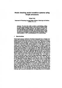
to transitions of component models it produces based on the modalities of the system MTS. As a running example consider the MTS N in Figure 3 with alphabet Σ = { a, b, c, d } and the alphabet distribution Γ = { Σ1 = { a, b }, Σ2 = { b, c, d } }. Conceptually, the algorithm projects N + onto the component alphabets and determinises each projection. The modality of a component MTS transition is set to required if and only if at least one of its corresponding transitions in the system MTS is required. The projections of N + on Σ1 and Σ2 are depicted in Figure 4, the deterministic versions of these projections are depicted in Figure 5, and the component MTS resulting from adding modalities to transitions is depicted in Figure 6. Note that the numbers in states of the deterministic MTS in Figures 5 and 6 correspond to the states of N as a result of determinisation. We now present a formal yet abstract distribution algorithm defined in terms of the subset construction for determinising LTS models [HU79] and the LTS distribution algorithm in [Ste06].

{9} {1,3}

a

{4}

d

b

{11}

{5,6,7} {1,2}

a {11,12}

b

c

{4}

b

{5,7}

c

b

{9,10}

{10}

(a) Projected onto Σ1

b

{12}

(b) Projected onto Σ2

Fig. 5. N + projected onto the local alphabets and determinised

Definition 11 (MTS distribution). Let M = hS, s0 , Σ, ∆p , ∆r i be an MTS S and Γ a distribution then the distribution of M over Γ is DIST MT [M ] = Γ p 0 r { M1 , . . . , Mn } where ∀i ∈ [1, n]Mi = hSi , si , Σi , ∆i , ∆i i and: – Si ∈ 2S where Si is reachable from the initial state following ∆pi . – s0i = CΣi (s0 ). [ t – (s, t, q) ∈ ∆pi ↔ q = { k ′′ ∈ CΣi (k ′ ) | k −→p k ′ }. k∈S t

– (s, t, q) ∈ ∆ri ↔ (s, t, q) ∈ ∆pi ∧ ∃k ∈ s · k −→r . When Γ is clear from the context we just write DIST MT S [M ] instead of S DIST MT [M ]. Γ Note that in component N1 of Figure 6 the required b transition from state { 9, 10 } to { 11, 12 } is a consequence of the required b transition from 9 to 11 and the maybe b transition from 10 to 12 in N . Had the transition from { 9, 10 } to { 11, 12 } in N1 been a maybe rather than required then the distribution would not be sound. Let N1′ be such component. N1′ allows an implementation as in Figure 5(a) but without the last b transition from { 9, 10 } to { 11, 12 }. We aba

b

acbad

b

refer to this implementation as I 1 : I 1 −→p 6−→. Let I 2 be the LTS in Figure 5(a). I 2 is actually an implementation of N2 . But I 1 k I 2 is not an implementation acbad

b

of N as I 1 k I 2 −→ p 6−→ and N −→ p −→r . Hence the need to make the b transition { 9, 10 } to { 11, 12 } required in order to ensure soundness. We now discuss soundness of MTS distributions as constructed in Definition 11. First, note that Definition 11 when applied to LTS is equivalent to Definition 8, that is the distribution constructed when the MTS is a deterministic LTS is, in effect, a distribution of the LTS. What follows is a sketch of the more general soundness proof. Theorem 2 (Soundness). Let M be a deterministic MTS and Γ a distribution such that M + is a distributable LTS over Γ , then the MTS distribution (Definition 11) is sound (as defined in Definition 10).

{9} {1,3}

a?

{4}

d

b

{5,6,7} {1,2}

a {11,12}

{11}

b

b

(a) Component N1 .

c?

{4}

{5,7}

b

c? {9,10}

{10}

{12}

b?

(b) Component N2

Fig. 6. Distribution of MTS in Figure 3

Proof. We need to prove that for any I1 , . . . , In such that Mi  Ii then M  ki∈[n] I. As refinement is a precongruence with regards to k meaning that if Mi  Ii for i ∈ [n] then ki∈[n] Mi  ki∈[n] Ii we just need to prove M  ki∈[n] Mi . Thus M  ki∈[n] Ii . We now prove M  ki∈[n] Mi . M + is distributable and the MTS components produced by DIST MT S [M ] are isomorphic, without considering the transitions’ modality, to the LTS components produced by DIST LT S [M + ]. So the parallel composition of the MTS component is isomorphic, again without considering the transitions’ modality, to the parallel composition of the LTS components. When the MTS components are created if, after the closure, there is a required transition then the component will have a required transition and so the composition may have a required transition where the monolithic MTS had a maybe transition. But any possible behaviour in the composed MTS is also possible in the monolithic MTS. Therefore the composed MTS is a refinement of the monolithic MTS. ⊓ ⊔ We now define modal consistency of transitions, which is a necessary condition for Definition 11 to produce complete distributions. We say that the modalities of an MTS M are inconsistent with respect to an alphabet distribution Γ when there is an action ℓ such that there are two traces w and y leading to two transitions with different modalities on ℓ (i.e. a required and a maybe ℓ-transition) and that for each component alphabet Σi ∈ Γ where ℓ ∈ Σi , the projection of w and y on Σi are the same. The intuition is that if M is going to be distributed to deterministic partial component models, then some component contributing to the ocurrence of the ℓ after w and y must have a different reached both points through different paths (i.e. w|Σi 6= y|Σi ). If this is not the case, then the distribution will have to make ℓ after w and y always maybe or always required. Definition 12 (Alphabet Distribution Modal Consistency). Let Γ be an alphabet distribution and M = hS, s0 , Σ, ∆r , ∆p i an MTS then M is modal w

ℓ

y

ℓ

consistent with respect to Γ iff ∀w, y ∈ Σ ∗ , ℓ ∈ Σ · M −→p −→r ∧ M −→p −→m implies ∃i ∈ [n] · ℓ ∈ Σi ∧ w|Σi 6= y|Σi

3 c?

1 a?

6

a?

d

4 2

c?

a?

b

5 c?

9 d

a?

7

8

b

11

c?

a

10

b?

12

Fig. 7. P : Modal Inconsistent MTS with respect to { { a, b }, { b, c, d } }

Consider model N from Figure 3. This MTS is modal consistent for Γ = ℓ w { Σ1 = { a, b }, Σ2 = { b, c, d } } as the only w, y and ℓ such that N −→p −→m y

ℓ

and N −→p −→m are ℓ = b, and w and y sequences leading to states 9 and 10 (for instance w = cabda and y = acbac). However, all sequences leading to 9 when projected onto Σ2 yield cbd while those leading to 10 yield cbc. Hence, consistency is satisfied. Now consider model P in Figure 7 (a modified version of N but with the a a following modalities changed: 5 −→m 8 and 6 −→m 9). P is not modal consistent with respect to Γ = { Σ1 = { a, b }, Σ2 = { b, c, d } }: Now there are w = acb y w a a and y = acbc such that N −→p −→m and N −→p −→m yet the only Σi that includes a is Σ1 and w|Σ1 = y|Σ1 = ab. A sound and complete distribution of P would require a deterministic component MTS for Σ1 = { a, b } that would either require a after ab or have a maybe a after ab. The former would disallow the implementation I1 of Figure 8(b) which in turn would make impossible having a component implementation I2 such that I1 kI2 yields I of Figure 8(a) which is a deterministic distributable implementation of P . Hence requiring a after ab would lead to an incomplete distribution. Choosing the latter would allow implementation I1 which would make the distribution unsound: In order to have implementations that when composed yield P + , an implementation with alphabet Σ2 = { b, c, d } bisimilar to Figure 8(c) is needed. However, such an implementation, when composed with I1 is not a refinement of P . Theorem 3 (Completeness). Let M be a deterministic MTS and Γ a distribution such that M + is a distributable LTS over Γ , and M is modal consistent then the MTS distribution (Definition 11) is complete (as defined in Definition 10). The proof of this theorem uses the following lemmas: Lemma 1. Let M, N be deterministic MTSs with α(N ) = α(M ) if ∀w ∈ Σ ∗ , t ∈ Σ w

w

– N −→p =⇒ M −→p t t w w – N −→p ∧ M −→p M ′ −→r =⇒ N ′ −→r

c

a

a

c

d b

(a) Implementation of Figure 7

d a

c

b

b

b c

b

(b) Component with Σ1 = { a, b } for P (c) Component with Σ2 = { b, c, d } for P + Fig. 8.

Then M  N . Lemma 2. Let M be an MTS and I ∈ DDI [M ]. For every Σi ∈ Γ let Mi and Ii be the components corresponding to Σi in DIST MT S [M ] and DIST LT S [I] w w respectively then ∀w ∈ Σi · Ii −→p =⇒ Mi −→p . S Proof (Theorem 3). Let DIST MT [M ] = { M1 , . . . , Mn }. We need to prove Γ that for every I ∈ DDI Γ [M ] there are Ii with i ∈ [n] where Mi  Ii and S [I] = { Q1 . . . Qn } and ki∈[n] Ii ≡ I. As I is distributable over Γ then DIST LT Γ ki∈[n] Qi ≡ I. Recall that the distribution algorithms produce deterministic components. Therefore we can use Lemma 1 to show that each MTS component is refined by its corresponding LTS component. Let Mi and Qi be the MTS and LTS components for Σi ∈ Γ . Every possible trace in Qi is possible in Mi (Lemma 2). Then the only way Qi is not a refinement of Mi is because there is some required behaviour in Mi that is not present in Qi . So lets suppose Mi 6 Qi , then z

t

z

t

∃z ∈ Σi∗ , t ∈ Σi such that Mi −→p T −→r ∧ Qi −→p Q 6−→. We now present an algorithm that creates, for every i ∈ [n], a new component Ii from Qi by adding the missing required transitions from Mi in order to get Mi  Ii . The algorithm iteratively takes a pair (Mi , Iij ), where Iij is the component Ii constructed up to iteration j, such that Mi 6 Iij and adds a required transition for a pair mirroring Mi structure. The structure of Mi has to be kept in the resulting Ii in order to avoid trying to add infinite required transitions due to a loop of required transitions in Mi . If the added transitions are part, and complete, a loop in Mi then that same loop will be created in Ii when the

3 c?

1 a?

d?

4 2

a

6

a?

5

b

c?

c?

9 d?

a

8

7

a

11

b

3 c

1

c?

10

a

4 a

12

b?

b

5

a

6

c

2

(b) I E .

(a) E Fig. 9.

algorithm adds the required transitions. Furthermore, the added transitions do not modify the composition (Lemma 3). Algorithm 1 Extension to each Qi to get a refinement of Mi Input: { (M1 , Q1 ), . . . , (Mn , Qn ) } Output: { I1 , . . . , In } I1 = Q1 ; . . . ; In = Qn ; while ∃i ∈ [n] · Mi 6 Ii do take (Mi , Ii ) · Mi 6 Ii ; z

t

z

t

take z ∈ Σi∗ · Mi −→p P −→r P ′ ∧ Ii −→ Q 6−→; u u if ∃u ∈ Σi∗ · Mi −→p P ′ ∧ Ii −→ Q′ then t ′ Q −→ Q ; else t Add a new state Q′ to Ii and then the transition Q −→ Q′ ; end if end while

As an example of how the algorithm works consider the MTS E in Figure 9(a), that is like N from Figure 3 only that the d transitions are maybe in E instead of required, and Γ = { Σ1 = { a, b }, Σ2 = { b, c, d } }. Let DIST MT S [E] = { E1 , E2 }. E1 is the same as component N1 in Figure 6(a). E2 is like component N2 in Figure 6(b) only that the d transition from { 5, 7 } to { 9 } is a maybe d transition. I E in Figure 9(b) is an implementation of E and DIST LT S [I E ] = { Q1 , Q2 } (Figure 10(a) and 10(b)). The algorithm takes { (E1 , Q1 ), (E2 , Q2 ) } and returns components I1 (I1 is the same as the LTS in Figure 5(a)) and I2 (I2 is in fact Q2 ). As E2  Q2 then the algorithm will not aba

b

aba

b

change Q2 so I2 = Q2 . E1 6 Q1 because E1 −→p −→r and Q1 −→p 6−→. The algorithm then adds the missing transition to Q1 and the result is I1 (I1 is the same as the LTS in Figure 5(a)). Now E1  I1 and the algorithm finishes. See how I1 k I2 ≡ Q1 k Q2 as the added b transition to Q1 in I1 does not appear in the composition because Q2 does not provide the needed synchronisation. Finally we prove that the algorithm finishes. As there are finite components it is sufficient to show that Mi  Iim with m finite where Iij is Ii after doing j additions of required transitions to Ii .

{1,3}

a

{4}

b

{5}

a

{6}

{1,2}

c

{4}

b

{5}

(b) Q2 .

(a) Q1 Fig. 10.

Each iteration adds a missing required t transition to a Iij that is present in Mi . If the required transition in Mi goes to P ′ and there is a u ∈ Σi∗ from Mi to P ′ such that u is possible in Iij leading to Q′ then the new transition goes to Q′ . Q′ is already present in Iij−1 and the algorithm never modifies possible transitions so any possible behaviour in Iij−1 is possible in Mi and the same stands for Iij . On the other hand, if P ′ is not reachable by a word that is possible in Iij then the added required transition goes to a new state. This procedure modifies Ii until all reachable required transitions in Mi not present in Ii are added. As loops of required transitions in Mi that have to be added to Ii are added preserving the loop structure then the iterations for component Mi can not be more than the amount of required transitions present in Mi . And this is done for every pair of components but as they are n the algorithm finishes. ⊓ ⊔ The following lemma is used in the proof of Theorem 3. For all i ∈ [n] Ii refines Mi and the added transitions do not modify the composition. Formally: Lemma 3. Let M be a deterministic MTS such that M + is distributable over Γ and modal consistent. Let I ∈ DDI [M ], DIST LT S [I] = { Q1 , . . . , Qn } DIST MT S [Mi ] = { M1 , . . . , Mn } and { I1 , . . . , In } the output of Algorithm 1 for { (M1 , Q1 ), . . . , (Mn , Qn ) }then: – ∀i ∈ [n] Mi  Ii . – ki∈[n] Ii ≡ ki∈[n] Qi (and therefore ki∈[n] Ii ≡ I).

4

Related Work

Distributed implementability and synthesis has been vastly studied for LTS for different equivalences notion like isomorphism, language equivalence and bisimulation [Mor98,CMT99,Ste06,HS05]. The general distributed implementability problem has not been studied for MTS. A component view of the system has been taken in the context of studies on parallel composition of MTS [BKLS09b], however such view is bottom-up: Given partial behaviour models of components, what is the (partial) behaviour of the system resulting of their parallel composition. The only notable example that takes a top-down approach is [KBEM09] A synthesis procedure is proposed that given system level OCL properties and UML scenarios, component partial behaviour models are automatically constructed such that their composition requires the behaviour required by system level properties and scenarios, and proscribed the behaviour not permitted by the same properties and scenarios.

In [QG08], MTS distribution is studied as a instance of more general contractbased formalism. The notion that corresponds to our definition of complete and sound MTS Distribution (see Definition 10) is called decomposability, Definition 3.8 [QG08]. Decomposability is a strictly stronger notion which requires all implementations of M to be captured by some distribution ki∈[n] Mi . Our definition only requires distributable implementations of M to be refinements of ki∈[n] Mi . In particular Figure 3, with transition from 6 to 9 changed to being only possible, is not distributable according to [QG08] but is according to our definition. Moreover, the distribution algorithm of [QG08] cannot handle examples such as Figure 3.3 in [Ste06] which can be handled by standard LTS distribution algorithms (and ours) by determinising projections.

5

Conclusions

In this paper we provide results that support moving from iterative refinement of a monolithic system models to component-wise iterative refinement. We present a distribution algorithm for partial behaviour system models specified as MTS to component-wise partial behaviour models given as sets of MTSs. We precisely characterise when the decomposition provided is sound and complete, we also discuss why the restrictions to the distribution problem (namely determinism, modal consistency and distributability of M + ) are reasonable, are unlikely to be avoidable for any sound and complete distribution method, and can be seen as a natural extension of the limitations of existing LTS distribution results. Future work will involve experimenting with case studies to assess the practical limitations imposed by the restrictions introduced to enforce completeness of distributions. We expect insights gained to allow for definition of more generally applicable sound but not complete distribution algorithms and elaboration techniques to support refinement of system models into models for which distribution algorithms exist.

References [BKLS09a] N. Beneˇs, J. Ket´ınsk´ y, K. G. Larsen, and J. Srba. Checking thorough refinement on modal transition systems is exptime-complete. ICTAC ’09, pages 112–126. Springer-Verlag, 2009. [BKLS09b] N. Beneˇs, J. Ket´ınsk´ y, K. G. Larsen, and J. Srba. On determinism in modal transition systems. Theor. Comput. Sci., 410(41):4026–4043, 2009. [CMT99] I. Castellani, M. Mukund, and P. S. Thiagarajan. Synthesizing distributed transition systems from global specification. In FSTTCS, pages 219–231, 1999. [DFFU07] N. D’Ippolito, D. Fishbein, H. Foster, and S. Uchitel. MTSA: Eclipse support for modal transition systems construction, analysis and elaboration. In eclipse ’07: Proceedings of the 2007 OOPSLA Workshop on eclipse technology eXchange, pages 6–10. ACM, 2007. [FBD+ 11] D. Fischbein, G. Brunet, N. D’Ippolito, M. Chechik, and S. Uchitel. Weak alphabet merging of partial behaviour models. TOSEM, pages 1–49, 2011.

[GP11]

Patrice Godefroid and Nir Piterman. Ltl generalized model checking revisited. STTT, 13(6):571–584, 2011. [HS05] K. Heljanko and A. Stefanescu. Complexity results for checking distributed implementability. In Proc. of the Fifth Int. Conf. on Application of Concurrency to System Design, pages 78–87. IEEE Computer Society, 2005. [HU79] John E. Hopcroft and Jeffrey D. Ullman. Introduction to automata theory, languages, and computation. Addison-Wesley, 1979. [KBEM09] I. Krka, Y. Brun, G. Edwards, and N. Medvidovic. Synthesizing partial component-level behavior models from system specifications. In ESEC/FSE ’09, pages 305–314. ACM, 2009. [LT88] K.G. Larsen and B. Thomsen. A modal process logic. In LICS’88, pages 203–210. IEEE Computer Society, 1988. [Mil89] R. Milner. Communication and Concurrency. Prentice-Hall, New York, 1989. [MK99] J. Magee and J. Kramer. “Concurrency - State Models and Java Programs”. John Wiley, 1999. [Mor98] Remi Morin. Decompositions of asynchronous systems. In CONCUR, pages 549–564, 1998. [QG08] Sophie Quinton and Susanne Graf. Contract-based verification of hierarchical systems of components. In Proceedings of the 2008 Sixth IEEE International Conference on Software Engineering and Formal Methods, SEFM’08, pages 377–381. IEEE Computer Society, 2008. [Ste06] Alin Stefanescu. Automatic Synthesis of Distributed Systems. PhD thesis, 2006. [Sto05] Martin Stoll. “MoTraS : A Tool for Modal Transition Systems”. Master’s thesis, Technische Universitat Munchen, Fakultat fur Informatik, August 2005. [SUB08] G. Sibay, S. Uchitel, and V. Braberman. Existential live sequence charts revisited. In ICSE’08, pages 41–50, 2008. [UKM04] S. Uchitel, J. Kramer, and J. Magee. Incremental elaboration of scenariobased specifications and behaviour models using implied scenarios. ACM TOSEM, 13(1), 2004.