This is a post-peer-review, pre-copyedit version of an article published in JLAMP Vol. 85, Issue 2 The final authenticated version is available online at: http://dx.doi.org/10.1016/j.jlamp.2015.11.006
Modelling and Analysing Variability in Product Families: Model Checking of Modal Transition Systems with Variability Constraints Maurice H. ter Beeka,⇤, Alessandro Fantechia,b , Stefania Gnesia , Franco Mazzantia a Istituto
di Scienza e Tecnologie dell’Informazione “A. Faedo”, CNR Via G. Moruzzi 1, 56124 Pisa, Italy b Dipartimento di Sistemi e Informatica, Università di Firenze Via S. Marta 3, 50139 Firenze, Italy
Abstract We present the formal underpinnings of a modelling and analysis framework for the specification and verification of variability in product families. We address variability at the behavioural level by modelling the family behaviour by means of a Modal Transition System (MTS) with an associated set of variability constraints expressed over action labels. An MTS is a Labelled Transition System (LTS) which distinguishes between optional and mandatory transitions. Steered by the variability constraints, the inclusion or exclusion of labelled transitions in an LTS refining the MTS determines the family’s possible product behaviour. We formalise this as a special-purpose refinement relation for MTSs, which differs fundamentally from the classical one, and show how to use it for the definition and derivation of valid product behaviour starting from product family behaviour. We also present a variability-aware action-based branchingtime modal temporal logic to express properties over MTSs, and demonstrate a number of results regarding the preservation of logical properties from family to product behaviour. These results pave the way for the more efficient familybased analyses of MTSs, limiting the need for product-by-product analyses of LTSs. Finally, we define a high-level modal process algebra for the specification of MTSs. The complete framework is implemented in a model-checking tool: given the behaviour of a product family modelled as an MTS with an additional set of variability constraints, it allows the explicit generation of valid product behaviour as well as the efficient on-the-fly verification of logical properties over family and product behaviour alike. Keywords: Model checking, Modal transition systems, Temporal logic, ⇤ Corresponding
author Email addresses:
[email protected] (Maurice H. ter Beek),
[email protected] (Alessandro Fantechi),
[email protected] (Stefania Gnesi),
[email protected] (Franco Mazzanti)
Preprint submitted to Elsevier
October 21, 2015
Product families, Variability 1. Introduction Software Product Line Engineering (SPLE) [31, 61] is by now a full-fledged software engineering approach aimed at developing, in a cost-effective manner, a family of software-intensive systems by systematic reuse. Individual products share an overall reference model or architecture of the product family, but they differ with respect to specific features. A feature is a (user-visible) increment in functionality of a product. SPLE reduces time-to-market, increases product quality, and lowers production costs. The common and variable parts of products are defined in terms of features and managing variability is about identifying the variation in a shared family model to encode exactly which combinations of features constitute valid products. The actual configuration of products during application engineering is then reduced to selecting desired options in the variability model. Hence, the overall production process is organised so as to maximise commonalities and at the same time minimise the cost of variations. Variability modelling and analysis of software-intensive systems traditionally focusses on structural rather than behavioural properties and constraints. It is important to model and analyse their variability also at the behavioural level, in order to provide a form of quality assurance. This was first perceived in the context of UML 2.0 [46, 69]. Consequently, Modal Transition Systems (MTSs) were recognised in [40] as a promising model to describe in a compact way all possible operational behaviour of the products of a product family. In a nutshell, an MTS [1] is an LTS that distinguishes between admissible (‘may’) and necessary (‘must’) transitions. Following [40], variants and extensions of MTSs were studied in order to elaborate a suitable formal modelling structure to describe variability in terms of behaviour, including modal I/O automata [52], variable I/O automata [55], and MTSs with logical variability constraints [4, 5, 36]. This triggered a growing interest in modelling behavioural variability, which led to the application of formal models different from MTSs, but still with a transition system semantics, including first and foremost the highly elaborated framework based on featured transition systems [26, 27], but also process-algebraic approaches [12–14, 42, 45, 67], Petri nets [59], and finite state machines [57]. As a result, behavioural analysis techniques like model checking [6, 23] became available for the verification of (temporal) logic properties of product families, resulting in special-purpose model checkers [15, 16, 25, 32]. In this paper, we focus on one such approach. We present the full formal underpinnings of a modelling and analysis framework, some of whose aspects were introduced in [4, 5, 15, 16]. It is based on a specific subset of MTSs, whose elements are equipped with an additional set of logical variability constraints expressed over actions. These constraints allow one to capture all common variability notions known from feature models [43, 49, 63], since it is well-known that plain MTSs cannot efficiently (in a compact way) model, e.g., the notions of alternative and mutually exclusive features. Considering the may transitions as 2
optional and the must transitions as mandatory, an MTS can be interpreted as a family of LTSs such that each family member corresponds to a specific selection of optional transitions. In this way, a single MTS can model a product family since it allows a compact representation of the family’s behaviour, by means of states and actions, shared by all products, and variation points, by means of may and must transitions, used to differentiate among products. A specific selection of labelled transitions respecting the variability constraints expressed over action labels, determines possible product behaviour (modelled as LTSs). In this paper, we formalise this for the first time as a special-purpose refinement relation for MTSs, which differs fundamentally from classical MTS refinement, and we show how to use it to formally define and derive valid (i.e., configurable) product behaviour starting from the behaviour of a product family. Subsequently, we recall v-ACTL, a variability-aware action-based branchingtime modal temporal logic that was introduced to reason over MTSs [15]. To this aim, it provides novel interpretations of some classical modal and temporal operators. In this paper, we demonstrate a number of results regarding the preservation of v-ACTL properties from family to product behaviour. These results pave the way for family-based analyses of MTSs, limiting the need for enumerative product-by-product analyses of LTSs. Based on model-checking techniques for v-ACTL, we updated the Variability Model Checker VMC [15, 16] in such a way that it now allows one to perform two kinds of behavioural variability analysis on a product family modelled as an MTS with additional variability constraints: 1. The actual set of valid product behaviour can explicitly be generated from the MTS and both the MTS and the resulting LTSs can be verified against a logical property expressed in v-ACTL; 2. A logical property can be verified directly over the MTS, relying on the fact that under certain syntactic conditions, validity over the MTS guarantees validity of the same property for all the family’s valid products (LTSs). Finally, we formally define the modal process algebra that VMC accepts as specification of an MTS and we illustrate the applicability of the overall framework and its associated tool by means of an example family of coffee machines. The paper is based on previous publications (in particular, [4, 5, 15, 16]), but it contains new material and results. The formal definition of refinement of MTSs has been completely revisited for the specific purpose of defining and deriving LTSs modelling valid product behaviour, which has required the introduction of new notions like consistent and valid products. The preservation by refinement of v-ACTL formulae has been formally defined and proved. The full syntax and semantics of the high-level modal process algebra used to specify MTSs in VMC has been defined and the associated set of variability constraints may now contain any Boolean expression over the action labels. The paper is organised as follows. After presenting a running product family example in Section 2, we introduce the modelling framework of MTSs with additional variability constraints in Section 3. In Section 4, we define the actionbased branching-time modal temporal logic, v-ACTL, for the formulation and 3
analysis of behavioural variability in MTSs. The associated model-checking tool, VMC, for the specification and verification of behavioural variability in product families modelled as MTSs is described in Section 5. Section 6 discusses related models and tools and, finally, Section 7 contains some concluding remarks. 2. Running Example of Variability in Product Families Throughout the paper, we will use a family of (simplified) coffee machines as running example, variants of which have been used in [4, 5, 8, 12, 14, 16, 17, 19, 27, 28, 36, 37, 42, 59]. It is described by the following list of requirements: 1. Each time a user desires a beverage, initially (s)he must insert a coin: either a euro, exclusively in case of coffee machines for the European market, or a dollar, exclusively in case of coffee machines for the Canadian market; 2. After having inserted a coin, the user has to be offered the option to choose whether or not (s)he wants sugar in her/his beverage, after which (s)he has to be offered to select a beverage; 3. The choice of beverages offered by a coffee machine may vary (the options being cappuccino, coffee, and tea), but every coffee machine must offer at least one beverage. Furthermore: (a) tea may only be offered by coffee machines for the European market; (b) whenever a coffee machine offers cappuccino, then it must offer coffee as well; (c) whenever a coffee machine offers coffee, then it either delivers always espresso or always regular coffee; 4. After the user has chosen her/his beverage, the coffee machine delivers it and, as soon as the user has taken her/his beverage, the coffee machine must return in its idle state. Note that these requirements contain both structural constraints, defining differences in configuration (in terms of features) among products, and operational constraints, defining the behaviour of products through admitted sequences (temporal orderings) of actions/operations (which implement features). An example of the former is the fact that every coffee machine must offer at least one beverage, but in a Canadian coffee machine this must be either coffee or cappuccino (and coffee), whereas an example of the latter is that a coin must have been inserted before a beverage can be chosen. To illustrate a number of technical definitions, mainly in the next section, we will use an even more simplistic family of coffee machines that deliver a coffee upon the insertion of either a euro or a dollar. 3. Modelling Behavioural Variability in Product Families Similar to earlier approaches based on variants of MTSs [36, 40, 52, 55], we use MTSs for describing in a compact and abstract way the behaviour of an entire product family and their underlying model of LTSs for describing individual product behaviour. 4
Definition 1 (LTS). A Labelled Transition System (LTS) is a tuple (Q, ⌃, q, ), where Q is a finite and non-empty set of states, ⌃ is a finite set of actions, q 2 Q is an initial state, and ✓ Q ⇥ ⌃ ⇥ Q is a transition relation. We sometimes a write q ! q 0 if (q, a, q 0 ) 2 and we call it an a-transition (from source q to 0 target q ). Definition 2 ((full) path). Let L = (Q, ⌃, q, ) be an LTS and let q 2 Q. Then, is a path from q if = q (empty path) or = q1 a1 q2 a2 q3 · · · with q1 = q and ai qi ! qi+1 for all i > 0 (possibly infinite path); its i-th state is denoted by (i) and its i-th action is denoted by {i}. A state q 2 Q is reachable (in L) if there exists a path from q to q, i.e., (i) = q for some i > 0. A state q 2 Q is final (a.k.a. a sink state) if it does not have outgoing transitions. An action a 2 ⌃ is reachable (in L) if there exists a path from q such that {i} = a, for some i > 0. A full path is a path that cannot be extended any further, i.e., it is infinite or it ends in a final state. The set of all full paths from q is denoted by path(q). We also say that a state (action) can be reached (occurs) in an LTS if it is reachable. An MTS is an LTS with a distinction among admissible (may) and necessary (must) transitions [53]. Definition 3 (MTS). A Modal Transition System (MTS) is a tuple (Q, ⌃, q, 3 , such that (Q, ⌃, q, 3 ) is an LTS (its underlying LTS) and 2 ✓ 3 . An MTS distinguishes the may transition relation 3 , expressing admissible transitions, and the must transition relation 2 , expressing necessary transitions. We somea a times write q !3 q 0 for (q, a, q 0 ) 2 3 and q !2 q 0 for (q, a, q 0 ) 2 2 and we sometimes call them may a-transition and must a-transition, respectively. In the sequel, we will refer to transitions in 3 \ 2 as optional transitions1 .
Note that any transition is thus either a must transition or an optional transition (and in any case it is by definition also a may transition). Definition 4 (must path). Let F be an MTS and let = q1 a1 q2 a2 q3 · · · be a non-empty full path in its underlying LTS. Then, is a must path (from q1 ) in ai F if qi ! is denoted by 2 . 2 qi+1 for all i > 0. A must path
Graphically, an MTS is represented as a directed edge-labelled graph, where nodes model states and edges model transitions; in addition, a small arrow indicates its initial state. Solid edges model necessary transitions (i.e., 2 ) while dotted edges model optional transitions (i.e., 3 \ 2 ). The edges are labelled with actions that are executed as the result of state changes. A sequence of state changes and the executed actions is a path in the graph; it is a must path if all edges involved are solid ones. 1 In
[40], these are called maybe transitions.
5
2
)
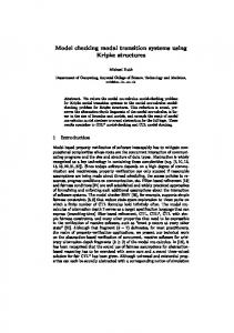
Example 1. Figure 1(a) depicts an MTS modelling a simplistic family of coffee machines: upon the insertion of either a euro or a dollar, a coffee is delivered. A number of LTSs that can be obtained by step-by-step refining (unfolding) its optional behaviour are depicted in Figs. 1(b)-1(l). In the sequel we will define precisely which of these are considered products of this family of coffee machines.
(a) MTS
(g)
(b)
(h)
(c)
(d)
(i)
(e)
(j)
(k)
(f)
(l)
Figure 1: (a)-(l) A family MTS and some potential product LTSs
3.1. Resolving Variability by Refinement An MTS thus describes the possible behaviour of a product family, including variability modelled through optional transitions, i.e., admissible (may), but not necessary (must) transitions (the dotted edges in Fig. 1(a)). The idea is that the family’s products, i.e., ordinary LTSs, can be obtained by resolving this variability. Resolving variability boils down to deciding for each particular optional behaviour whether or not it is to be included in a specific product. This leads to the need for a notion of conformance that defines whether the product behaviour of an LTS conforms to the required family behaviour described by the MTS or not. Traditionally, implementations of an MTS are LTSs that capture the idea of refining a partial description into a more detailed one, reflecting increased knowledge on the admissible (but not necessary) behaviour. We know from [40] 6
that the usual (strong and weak refinement) semantics over MTSs are not capable of capturing a notion of conformance that is suitable for SPLE. This is because even if only the observable behaviour is considered, it can still be the case that MTS behaviour is not preserved consistently throughout LTSs, in the sense that the decision to include (i.e., implement) optional transitions can vary from one occurrence to the other (cf. Examples 4 and 5). In this section, we show how we can nevertheless make use of the classical notions of refinement and implementation among transition systems in our definition of a behavioural conformance for MTSs. This conformance relation should match the SPLE notion that each product of a product family is a refinement of that family, based on the understanding that an LTS (product behaviour) conforms to the MTS (family behaviour). Definition 5 (refinement). An MTS Fp = (Qp , ⌃, q p , p3 , p2 ) is a refinement of an MTS F = (Q, ⌃, q, 3 , 2 ), denoted by F Fp , if and only if there exists a refinement relation R ✓ Q ⇥ Qp such that (q, q p ) 2 R and for any a 2 ⌃ and for all (q, qp ) 2 R, the following holds: a
1. whenever q !2 q 0 , for some q 0 2 Q, then there exists a qp0 2 Qp such that a qp !2 qp0 and (q 0 , qp0 ) 2 R, and a
2. whenever qp !3 qp0 , for some qp0 2 Qp , then there exists a q 0 2 Q such a that q !3 q 0 and (q 0 , qp0 ) 2 R. Intuitively, Fp refines F if any must transition of F exists in Fp and every may transition in Fp originates from F. Obviously, an MTS in which 3 ✓ 2 (i.e., 2 = 3 ) is actually an LTS. Note that an a-transition of an MTS that is present in all its refinements is by definition a must transition of the MTS. Hence, an a-transition that is present in some, but not not all, of its refinements is a may transition. Obviously, it cannot be the case that an a-transition is not present in any of its refinements. Since all must transitions are preserved by refinement, so are the must paths. The symmetric, for paths consisting of only may transitions, is also true. Proposition 1. Let F and Fp be MTSs such that F 1. If
Fp . Then:
= q1 a1 q2 a2 q3 · · · is a must path of F, then there exists a must path 0 0 = qp1 a1 qp2 a2 qp3 · · · of Fp such that (qi , qp0 i ) 2 R for all i > 0; p 0 0 2. If p = qp1 a1 qp2 a2 qp3 · · · is a path of Fp , then there exists a path = q1 a1 q2 a2 q3 · · · of F such that (qi , qp0 i ) 2 R for all i > 0.
Definition 5 thus also defines when an LTS is a refinement of an MTS. LTSs that are refinements of an MTS F are called implementations of F. Definition 6 (implementation). An LTS Fp is an implementation of an MTS F if and only if F Fp . We will refer to the refinement relation between an MTS and an LTS as an implementation relation. The set of all implementations of F is denoted by I(F). 7
Given an MTS F, the refinement relation induces a preorder over MTSs with top MTS F, and whose bottom elements are the LTSs that are implementations of F.
Example 2 (Example 1 continued). The LTSs depicted in Figs. 1(b)-1(k) are implementations of the MTS in Fig. 1(a). The LTS in Fig. 1(l) is not, because it does not contain the only must transition of the MTS even though its source state is reachable. The implementation relation allows LTSs with unreachable states (as an effect of pruning may transitions). Since, also for verification purposes, we are interested only in the reachable states representing effectively possible behaviour, we restrict our attention to implementations without unreachable states. Moreover, the number of implementations is in general infinite, because we can apply any number of unfoldings (and even duplications) similar to the ones that resulted in the LTS in Figs. 1(g)-1(i). In fact, in [36, 40] it was noted that refinement need not preserve an MTS’s branching structure. In the SPLE context, instead, we believe it useful to have a simpler notion of refinement which always preserves the original branching structure (up to the removal of unreachable states) of the MTS in the products, corresponding to the modellers’ intuition, and which gives to the implementations the choice of just turning dotted edges into solid edges or removing them altogether. Hence, before removing unreachable states, any implementation has exactly the same states as the MTS. As we will see shortly, this stricter notion of refinement has the immediate advantage of leading to a limited set of product behaviour. For our purposes, the minimal products thus suffice, so we will consider the minimal of all possible implementations according to strong bisimulation equivalence [58]. Definition 7 (bisimulation). Let L1 = (Q1 , ⌃1 , q 1 , 1 ) and L2 = (Q2 , ⌃2 , q 2 , 2 ) be two LTSs. We say that L1 and L2 are (strongly) bisimilar, denoted by L1 ⇠ L2 , if and only if there exists a (strong) bisimulation equivalence B ✓ Q1 ⇥ Q2 such that (q 1 , q 2 ) 2 B and for any a 2 ⌃ and for all (q1 , q2 ) 2 B, the following holds: a
a
1. whenever q1 ! q10 , for some q10 2 Q1 , then 9 q20 2 Q2 such that q2 ! q20 and (q10 , q20 ) 2 B, and a a 2. whenever q2 ! q20 , for some q20 2 Q2 , then 9 q10 2 Q1 such that q1 ! q10 and (q10 , q20 ) 2 B.
Definition 8 (product). An LTS Fp = (Qp , ⌃, q p , p ) is a product of an MTS F if and only if Fp is the minimal (w.r.t. the number of states and transitions) element of one of the classes of equivalences induced by strong bisimulation over I(F). The set of all products of F is denoted by Ip (F). This definition cuts out the LTSs with unreachable states and with useless unfoldings and duplications. Theorem 1. If L is the minimal element of a class of bisimulation equivalent LTSs, then all its states are reachable. 8
TO DO
Proof. Assume that L is minimal and that it has an unreachable state q. Consider the LTS L0 obtained from L by recursively navigating all its transitions. Then L0 is bisimulation equivalent to L by construction, but by definition it contains no state corresponding to q. Hence L is not minimal. Example 3 (Example 1 continued). The LTSs depicted in Figs. 1(b)-1(e), 1(j), and 1(k) are thus products of the MTS in Fig. 1(a). The LTS in Fig. 1(f ) is not, because it has more elements than the bisimilar LTS in Fig. 1(b). Likewise the LTSs in Figs. 1(g) and 1(h), which have more elements than the bisimilar LTS in Fig. 1(e), are not, and neither is the LTS in Fig. 1(i), which is bisimilar to the smaller LTS in Fig. 1(d). We adopt the same (often implicit) assumption that underlies the behavioural variability models based on MTSs [4, 5, 36, 40], I/O automata [52, 55], LTSs [45], featured transition systems [26–29], and mCRL2 [17] mentioned in Section 1, viz. an action models a piece of functionality (a feature, if you like). Now, recall that an MTS models the variability of a product family through its optional transitions, which need to be resolved to obtain the family’s products. This means that it must be decided whether or not an optional transition of an MTS should occur in an LTS modelling a product. For our application in SPLE, we need variability to be resolved in a consistent way, i.e., the choice of ‘implementing’ or ‘not implementing’ a transition in a product must be consistent throughout the product. This is because it reflects the fact that a functionality (or a feature) either is or is not present in a product, independently of its behavioural context. Informally, this notion of consistency states the following. Given an MTS and an LTS modelling one of its products, we want that for all actions a, either all or none of the a-transitions in the MTS occur (i.e., are ‘implemented’) as must a-transitions in its product. Two illustrative examples follow the formal definition. Definition 9 (consistent product). Let F = (Q, ⌃, q, 3 , 2 ) be an MTS and Fp = (Qp , ⌃, q p , p ) be a product of F, i.e., Fp 2 Ip (F), through the implementation relation R ✓ Q ⇥ Qp . Then, Fp is said to be consistent (with F) if and only if for all a 2 ⌃, the following holds: • if there exist a (q, a, q 0 ) 2 3 and a (qp , a, qp0 ) 2 p , with (q, qp ) 2 R and (q 0 , qp0 ) 2 R, then for all (r, a, r0 ) 2 3 for which there exists an rp 2 Qp such that (r, rp ) 2 R, there must exist an rp0 2 Qp such that (rp , a, rp0 ) 2 p and (r0 , rp0 ) 2 R. The set of all consistent products of F is denoted by Icp (F). Example 4 (Example 1 continued). The LTSs depicted in Figs. 1(j) and 1(k) are not consistent products of the MTS in Fig. 1(a). This can be seen as follows. First recall that the consistency assumption states that whenever it is decided to ‘implement’ the e-transition in a product, then this has to be done in a consistent way. In this particular example, this means that whenever the e-transition is implemented from their initial states, as is currently the case in both products, 9
(a) MTS modelling the family and. . .
(b) . . . an LTS modelling one of its products
Figure 2: (a)-(b) Modelling the family of coffee machines and a (Canadian) coffee machine
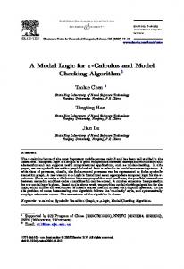
then it should also be implemented from the states that are reached after this action e and the action K have each occurred once, which is however not the case in Figs. 1(j) and 1(k). The LTSs depicted in Figs. 1(b)-1(e) are consistent products. In the next section, we will deal with the (undesired) trivial product in Fig. 1(b) and we will discuss whether the one in Fig. 1(e) is desired. A convenient result of the consistency assumption is that it makes the number of products finite. In Example 4, e.g., we have seen that the LTS depicted in Fig. 1(k) is not a consistent product of the MTS in Fig. 1(a) and the same obviously holds for any further unfolding of that MTS. Example 5. Now consider the MTS depicted in Fig. 2(a). It is an attempt to model all possible (product) behaviour conceived for the example family of coffee machines from Section 2. Note that it has variation points to model the choices among the different types of coin, beverage, and coffee. Moreover, note that the MTS allows each of the beverages to be delivered either with or without sugar. Without the requirement for consistent product behaviour, a product that can deliver coffee only without sugar would be allowed. An example of such an undesired product is depicted in Fig. 3(a): as soon as the user chooses for a sugared beverage, (s)he has less options than if (s)he had chosen for an unsugared beverage. The LTSs in Figs. 2(b) and 3(b) instead model consistent Canadian and European products, respectively. In [18], consistency is guaranteed in a different way (and called persistency). They define so-called parametric MTSs, where it is allowed to choose in a consistent (persistent) way whether or not to implement a transition in a product by using parameters with a priori fixed (Boolean) values that settle this choice for the entire product.
10
(a) LTS of an inconsistent (European) product
(b) LTS of a European coffee machine
Figure 3: (a)-(b) Modelling products of the family of coffee machines
3.2. Deriving Products from Product Families The products of a family modelled by an MTS are thus LTSs that are obtained by resolving the variability inherent to MTSs. In Section 3.1, we have seen how to resolve this variability by means of semantic definitions based on refinement that are common in the literature on MTSs. However, for our specific purpose of applying MTSs in SPLE, an operational syntactic definition of derivation exists. It is presented in this section and it is the one actually implemented in our VMC tool that will be discussed in Section 5. Intuitively, in each LTS modelling a product of an MTS, all must transitions of the MTS are included, together with a subset of its optional transitions. As before (cf. Def. 9), we assume that the choice of including an optional transition needs to be consistent. More formally, a derived product LTS is obtained from an MTS in the following way. The LTS has the same set of actions and the same initial state, but it contains a subset of the set of states and a subset of the set of transitions such that (i) all its states are reachable from the initial state, (ii) all must transitions of the MTS are included in the LTS, except of course for those must transitions whose source states are not reachable in the LTS, and (iii) for any action a, whenever an a-transition of the MTS is included in the LTS, then any other (optional) a-transition in the MTS (from a state that is reachable in the LTS) is also included. Definition 10 (derived product LTS). Let F = (Q, ⌃, q, 3 , 2 ) be an MTS. Then, the set { Pi = (Qi , ⌃, q, i ) | i > 0 } of derived product LTSs of F, denoted by PF , is obtained from F by considering each pair (Qi , i ), with Qi ✓ Q and i ✓ 3 , such that the following holds: 1. every q 2 Qi is reachable in Pi ; 2. there exists no (q, a, q 0 ) 2 2 \ i such that q 2 Qi ; 3. for any a 2 ⌃, whenever (p, a, p0 ) 2 3 \ i , then for all q 2 Qi such that (q, a, q 0 ) 2 3 it must be the case that also (q, a, q 0 ) 2 i . 11
The following example illustrates the reason for the first two requirements in Def. 10; the need for the third requirement is to guarantee consistency. Example 6 (Example 1 continued). The set of derived product LTSs of the MTS in Fig. 1(a) that is generated by Def. 10 consists of the LTSs depicted in Fig. 1(b)-1(e). Note that the LTS in Fig. 1(f ) is not a derived product LTS of this MTS because it contains an unreachable state, while none of the LTSs in Figs. 1(g)-1(k) can of course be a derived product LTSs of the MTS since they contain more states than the MTS. The LTS in Fig. 1(l), finally, is not a derived product LTS because it does not contain the only must transition of the MTS even though its source state is reachable. We now show that Def. 10 is an alternative for the definition of consistent products (cf. Def. 9). Theorem 2. Let F be an MTS. The set of all derived product LTSs of F equals, modulo bisimulation, the set of consistent products of F: PF ' Icp (F) (i.e., every derived product LTS is the representative of an equivalence class whose minimal element is a consistent product and, conversely, every consistent product is equivalent modulo bisimulation to a derived product). Proof. Let F = (Q, ⌃, q, 3 , 2 ) and let Fp = (Qp , ⌃, q p , p ) be a derived product LTS of F. We start by proving that Fp is an implementation of F, i.e., we prove that Fp 2 I(F). From Def. 10 it follows directly that (i) all states that are maintained in Fp maintain also their outgoing must transitions and (ii) p may include further transitions that originally were optional in F. These two statements correspond to the definition of refinement, which means, since Fp is an LTS, that we can now prove that Fp is indeed an implementation. First, since a product of an MTS is the minimal element of the equivalence class induced by bisimulation over I(F), Fp is bisimilar to a product of F. Subsequently, requirement 3 of Def. 10 guarantees the consistency of Fp . On the other hand, suppose that we have a consistent product Fp of F that is not bisimilar to any derived product LTS of F. This means that the class of the partition over I(F), induced by bisimulation equivalence, that contains Fp , contains no derived product LTSs. The implementations of F, due to the refinement relation, maintain all must transitions and a subset of the optional transitions. By the consistency requirement, if an optional a-transition is not included in a product, neither are all other a-transitions. Hence, an equivalence class made of consistent implementations can be uniquely characterised by a subset of the optional transitions of F. Moreover, an equivalence class made of derived products can be uniquely characterised by its subset of preserved (included) optional transitions of F, which could not have been chosen in the derivation process. However, since all pairs of subsets Qi ✓ Q and i ✓ 2 [ 3 , respecting consistency, are considered in a derivation, it cannot be the case that the above subset of preserved optional transitions is not chosen in a derivation. Hence, every consistent product is bisimilar to an implementation. 12
From Def. 10, it becomes immediately clear that an MTS has at most 2n derived product LTSs, where n is the number of differently labelled optional transitions in the MTS (because each such set of transitions in 3 \ 2 labelled with the same action is either absent or present in a product LTS). 3.3. Modelling Additional Variability Constraints We have just seen that the MTS depicted in Fig. 2(a) has several variation points to model the choices among the different types of coin, beverage, and coffee prescribed by the requirements for a family of coffee machines in Section 2. However, also its underlying LTS (obtained by turning all optional transitions into must transitions) is a consistent product, even though it satisfies neither requirement 1 nor requirements 3(a-c). This is inherent to the use of MTSs for capturing the behaviour of product families: while capable of faithfully modelling some degree of optional or mandatory behaviour that may or must, respectively, be preserved in its products (LTSs), an MTS cannot efficiently model the constraints regarding alternative (neither ‘or’ nor ‘xor’) behaviour nor regarding the so-called excludes and requires cross-tree constraints known from feature models [4, 43, 49]. Such constraints can express the fact that the presence of a feature (mutually) excludes or, on the contrary, requires the presence of another feature. Their formal definitions follow shortly. The reason that plain MTSs cannot efficiently model these constraints in a compact way resides in the fact that the decision whether to preserve an optional transition of an MTS in a product (LTS) or not, can be made independently of the decision whether or not to preserve another optional transition of the MTS, as is illustrated in the following example. Example 7 (Example 1 continued). The informal description of the simplistic family of coffee machines modelled by the MTS in Fig. 2(a) (“upon the insertion of either a euro or a dollar, a coffee is delivered”) is of course rather vague. The coffee machine modelled by the LTS in Fig. 1(b) is arguably not an intended product of the family, but what about the products that allow to insert only dollars (Fig. 1(c)), only euros (Fig. 1(d)), or to interchange the insertion of both (Fig. 1(e)): are these to be considered valid products? Most real-world coffee machines deliver coffee exclusively upon the insertion of one type of coin, e.g., euros in Europe and dollars in Canada. Note that a simple constraint requiring product LTSs to contain either the $-transition or the e-transition would suffice (i.e., only the LTSs in Figs. 1(c) and 1(d) would model valid products). A single MTS, possibly with a new initial state, could of course join the LTSs depicted in Figs. 1(c) and 1(d), at the cost of duplicating the K-transition, but this would be highly inefficient and not at all compact in case of a family that should accommodate separate products for numerous different coins (e.g., $, e, £, U) and in case of more rich product behaviour (e.g., coffee, tea, cappuccino) that is for a large part shared among the various products (e.g., sugar, take cup) but with subtle variations (e.g., pour milk only in case of cappuccino). In [4, 5] we presented a preliminary solution to cope with this incapacity of 13
covering all common variability constraints, which we now extend significantly2 . We associate with an MTS modelling a product family a set of variability constraints that must be taken into account when deriving the set of product LTSs. Recall that an action is reachable in an LTS if there is a path in that LTS (i.e., starting from its initial state) on which it is executed (occurs). Definition 11 (variability constraints). Let L = (Q, ⌃, q, ) be an LTS and let ai 2 ⌃ for all i. The following variability constraints on actions from ⌃ may be defined over L, for m 2 and n 3: a1 ALT · · · ALT am : precisely one among the actions a1 , . . . , am is reachable in L; (¬)a1 OR · · · OR (¬)am : at least one among the conditions on actions a1 , . . . , am holds, i.e., ai is (not) reachable in L; a1 EXC a2 : at most one of the actions a1 and a2 is reachable in L; a1 REQ a2 : action a2 must occur in L whenever a1 is reachable in L; a1 REQ (a2 ALT · · · ALT an ) : precisely one among the actions a2 , . . . , an is reachable in L if a1 is reachable in L; a1 REQ (a2 OR · · · OR an ) : at least one among the actions a2 , . . . , an is reachable in L if a1 occurs in L. Note that ALT can also be expressed in terms of OR and EXC. Moreover, since the most recent extension in [8], implemented in VMC v6.2 (cf. Section 5), allows the ‘OR’ constraint to contain either ai (as before) or its negation ¬ ai , we can express any Boolean function over ⌃ in its conjunctive normal form. We nevertheless choose to keep the specific variability constraints introduced in Def. 11 because they reflect prominent constraint relations in feature modelling [43, 49]. We hope that this eases the uptake of our framework by SPL practitioners. We now define which consistent products (derived product LTSs) of an MTS with an associated set of variability constraints are to be considered valid products of the product family modelled by that MTS. Definition 12 (valid product). Let F = (Q, ⌃, q, 3 , 2 ) be an MTS with a set V of variability constraints (on actions from ⌃), and let Pi 2 Icp (F) be a consistent product of F. Then, Pi is a valid product of F with variabiliy constraints V if and only if Pi satisfies all variability constraints in V. Example 8 (Example 1 continued). Given the MTS depicted in Fig. 1(a) extended with the set V = {e ALT $} of variability constraints, its only valid products are the LTSs depicted in Figs. 1(c) and 1(d). 2 In [4, 5] we did not consider the so-called ‘OR’ constraint among actions, nor did we consider any n-ary constraints or the combined constraints involving ‘REQ’. The possibility to negate some of the action literals in the ‘OR’ constraint is a novelty that we introduced in [8].
14
Example 9 (Example 5 continued). For the family modelled by the MTS in Fig. 2(a), we can now characterise its set of valid products (coffee machines) as precisely those product LTSs that can be derived from the MTS according to Def. 9 and satisfy each of the following variability constraints: 1. 2. 3. 4. 5.
euro ALT dollar; cappuccino OR coffee OR tea; dollar EXC tea; cappuccino REQ coffee; coffee IFF (pour espresso ALT pour regular).
It is easy to verify that the consistent European product described by the LTS in Fig. 3(b) satisfies each of the above constraints. Hence, it models a valid (European) product. Recall from Example 5 that the one in Fig. 3(a) does not. Summarising, we thus propose to complement an MTS with a set of variability constraints in order to obtain a model capable of expressing families of LTSs and with characteristics that make it suitable for SPLE. Given this behavioural (semantic) model, we also need a logic that can be interpreted over it to be able to address the problem of checking properties over product families specified as MTSs (with additional variability constraints). In the next section, we present a suitable logic. 4. v-ACTL: A Logic for Expressing and Analysing Variability In this section, we first present a logic that allows one to reason over MTSs with variability constraints and which moreover provides a semantics for the latter, thus allowing us to refine the notion of valid products of an MTS with an associated set of variability constraints. Then, we study the preservation of properties from MTSs to their valid products, which results in the identification of two fragments of the logic which are such that all formulae expressed in them, and which hold for an MTS, preserve their validity for all valid products (LTSs). We introduce variability-aware ACTL (v-ACTL) as a logic, interpreted over MTSs, in which several logics that we introduced over the years culminate [4, 5]. The result is an action-based branching-time temporal logic for variability in the style of the action-based logic ACTL [33, 41]. More precisely, next to the standard operators of propositional logic, v-ACTL contains the classical box and — by duality — diamond modal operators, the existential and universal path quantifiers, and the (action-based) F (‘eventually’) and — by duality — G (‘globally’) operators. Furthermore, for the box, diamond, and F operators, v-ACTL also contains ‘boxed’ variants; these can be distinguished in a logic over MTSs by taking into account the specific modality (may or must) of the involved transitions and paths (e.g., requiring a path to consist of must transitions only). In particular, v-ACTL is a simplification of the logic available in the VMC tool that we will present in Section 5 [15] by leaving out the (weak) Until operators and including directly the F operator. The reason for limiting ourselves
15
to these two temporal operators in this paper is threefold3 . First, the resulting logic suffices for specifying the additional variability constraints from Def. 11. Second, it allows a more concise presentation of the forthcoming results on preservation by refinement in Sections 4.2 and 4.3. Third, it suffices for specifying a considerable number of interesting properties for product families in the presence of variability. v-ACTL defines action formulae (denoted by ), state formulae (denoted by ), and path formulae (denoted by ⇡). Definition 13 (syntax of action formulae). Action formulae are built as follows over a set A of atomic actions {a, b, . . .}: true | a | ¬
::=
|
^
Action formulae are thus Boolean compositions of actions. As usual, false abbreviates ¬ true, _ 0 abbreviates ¬(¬ ^ ¬ 0 ), and =) 0 abbreviates 0 ¬ _ . Definition 14 (semantics of action formulae). The satisfaction of an action formula by an action a, denoted by a |= , is defined as follows: a |= true always holds a |= b iff a = b a |= ¬ a |=
^
iff a 6|= 0
iff a |=
and a |=
0
Definition 15 (syntax of v-ACTL). The syntax of v-ACTL is: ::= ⇡
::=
true | ¬ F
| F
2
|
^
| [ ]
| F{ }
| [ ]2
2
| F { }
| E ⇡ | A⇡
Intuitively, the specificity of the ‘boxed’ variants of the respective classical modal and temporal operators can be understood as follows: [ ]
: in all next states reachable by a may transition executing an action satisfying , holds;
[ ]2
: in all next states reachable by a must transition executing an action satisfying , holds;
F
: there exists a future state in which
holds;
3 The extended version of v-ACTL as implemented in VMC contains also the least and greatest fixed-point operators, which provide a semantics for recursion used for “finite looping” and “looping”, respectively, as in [50], as well as no less than eight versions of the Until operator, based on combinations of action-based, weak (a.k.a. unless), and ‘boxed’ Until variants. The latter variants distinguish between may and must versions of the involved transitions and paths, similar to [ ]2 , h i2 , F 2 , and F 2 { }.
16
F2
: there exists a future state in which state are must transitions;
F{ }
holds and all transitions until that
: there exists a future state, reached by an action satisfying , in which holds;
F 2 { } : there exists a future state, reached by an action satisfying , in which holds and all transitions until that state are must transitions. Some further operators can be derived as usual. First, h i abbreviates ¬ [ ] ¬ : a next state exists, reachable by a may transition executing an action satisfying , in which holds. Second, h i2 abbreviates ¬ [ ]2 ¬ : a next state exists, reachable by a must transition executing an action satisfying , in which holds. Third, AG abbreviates ¬EF ¬ : in all states on all paths, holds. The formal semantics of v-ACTL is given by MTSs without additional variability constraints. Recall from Def. 2 that a full path is a path that cannot be extended any further, i.e. it is infinite or it ends in a final state. Definition 16 (semantics of v-ACTL). Let (Q, A, q, 3 , 2 ) be an MTS, with q 2 Q, and let be a full path. The satisfaction relation |= of v-ACTL is: q |= true always holds; q |= ¬ q |=
^
q |= [ ]
q |= [ ]2
iff q 6|= ; 0
iff q |=
a
iff for all q 2 Q such that q !3 q 0 and a |= , we have q 0 |= ; a
iff for all q 0 2 Q such that q !2 q 0 and a |= , we have q 0 |= ;
q |= A ⇡ iff for all |= F 2
;
0
0
q |= E ⇡ iff there exists a |= F
0
and q |=
0
2 path(q) :
iff there exists a j
iff there exists a j
|= F { }
|= F 2 { }
2 path(q) such that 0
0
|= ⇡;
|= ⇡;
1 such that (j) |= ; 1 such that (j) |=
iff there exists a j iff there exists a j
and 8 1 i < j :
( (i), {i}, (i + 1)) 2 2 ; 1 such that {j} |= and (j + 1) |= ; 1 such that {j} |=
and (j + 1) |= ,
and for all 1 i j : ( (i), {i}, (i + 1)) 2
2
.
v-ACTL thus interprets some classical modal and temporal operators in two different ways by explicitly considering the may and must modalities of the transitions and paths of the semantic model of MTSs. 4.1. Analysis in the Presence of Variability We recall from Section 3.3 that an MTS model of a product family is complemented with a set of variability constraints that an MTS otherwise cannot capture, i.e., the constraints regarding alternative (both ‘or’ and ‘xor’) behaviour and regarding the excludes and requires cross-tree constraints of feature models. 17
It is now possible to give a concise logical characterisation of all variability constraints introduced in Def. 11 by noting that the ‘reachability of an action a’ in a (product) LTS can be expressed by the formula EF 2 {a} true (or simply EF {a} true, since the interpretation of the boxed variant of EF collapses on the classic interpretation in the case of LTSs). Let { ai | 1 i n } be a set of actions. Then, the variability constraints from Def. 11 can be captured with the following v-ACTL formulae, with m 2 and n 3: W V a1 ALT · · · ALT am : 1im ((EF 2 {ai } true) 1j6=im (¬ EF 2 {aj } true)); W (¬)a1 OR · · · OR (¬)am : 1im (¬)EF 2 {ai } true; a1 EXC a2 : ¬ ((EF 2 {a1 } true) ^ (EF 2 {a2 } true));
a1 REQ a2 : (EF 2 {a1 } true) =) (EF 2 {a2 } true); 2 a1 REQ (a2 ALT · · · ALT W an ) : (EF2 {a1 } true)V=) ( 2in (EF {ai } true) 2j6=in (¬ EF 2 {aj } true)); W a1 REQ (a2 OR · · · OR an ) : (EF 2 {a1 } true) =) 2in (EF 2 {ai } true).
Now that all variability constraints are formalised in v-ACTL, we can refine the definition of a valid product (LTS) (cf. Def. 12 from Section 3.3). Let F = (Q, ⌃, q, 3 , 2 ) be an MTS with a set V of variability constraints expressed in v-ACTL. Then, the set of all valid products (LTSs) of the MTS F with variability constraints V, denoted by Ivp (F, V), is defined as follows: Ivp (F, V)
= '
{ Pi 2 Icp (F) | Pi |=
{ Pi 2 PF | Pi |=
for all
for all
2V}
2 V },
where ' denotes equality modulo bisimulation (cf. Theorem 2). Figure 4 illustrates the various definitions involved in the stepwise refinement of an MTS F into LTSs, among which its unique valid product with respect to the variability constraint V = {a REQ c}. Note that since LTSs contain only must transitions, when v-ACTL formulae are verified over products, the ‘boxed’ operators of v-ACTL simply collapse onto their classic interpretations. Apart from verifying variability constraints, v-ACTL can now be used to verify (temporal) logic properties of product families and of all their products. To this aim, we note that it is not always easy to interpret the result of verifying a v-ACTL formula over an MTS, since in general a v-ACTL formula that is true for an MTS, may be false for some of its implementations, and vice versa, as the following examples illustrate. Example 10 (Example 5 continued). The property ‘Whenever a coffee is selected, a coffee is eventually delivered’ can be formulated as: AG [coffee] AF 2 {pour espresso _ pour regular } true 18
MTS Refinements of
a
=
b a b
a
a
b a
a
b
b
c
c
b c
b
a b c
c
b
Implementations (LTS)
c a
b
b
a b
b
a
b
b b
c
c
a
a
b
a b
Minimal Elements (Products)
c a
b
b
a
b a
b
b
c
b
a
a
a
a
b a
a
a
a
b
c
Minimal, Consistent Products (Derived Products)
a
c
Valid Products a
b
b
c
a b
c
a
a b
b c
b
Constraints = { a REQ c }
b
a a c
b
c
Figure 4: A universe of MTS refinements
19
b
Note that we use the ‘boxed’ variant of the classic F operator to express the fact that eventually coffee is actually poured. As a result, this formula does not hold for the MTS modelling the family of coffee machines depicted in Fig. 2(a), but it does hold in the product LTSs depicted in Figs. 2(b) and 3(b), i.e. the above formula expresses a property that holds for these Canadian and European coffee machines. Example 11. Consider the MTSs F and Fp in Fig. 5(a). Clearly F Fp with (q, qp ) 2 R. Since there is no must transition from q in F, it is trivially the case that q |= [a]2 . However, from the must transition (qp , a, qp0 ) in Fp and the fact that qp0 |= ¬ , it follows immediately that qp 6|= [a]2 .
(b) F 0
(a) F (top) and Fp (bottom)
(c) Fp0
Figure 5: (a)-(c) Counterexamples for preservation by refinement and by live MTS
In the next sections, we will discuss the inheritance of analysis results from families to products. We study under which conditions a v-ACTL property that is true for an MTS is also true for its product LTSs, and likewise for the preservation of properties that are false. The final aim is to achieve a specific type of family-based verification [66]: once a property is verified for a family model, one knows that the result also holds for any of its product models, without the need to explicitly verify the property over the products (as opposed to product-based verification, in which every product has to be examined individually). The above examples provide some intuition for the reason why, in general, it might not be the case that the result of a v-ACTL formula is preserved from an MTS to its product LTSs. Already in [5], it was noted that the refinement relation is similar to the well-known notion of simulation between LTSs, and hence the classical result of preservation of the universal fragment of CTL by simulation [24] can be reused for v-ACTL. In the following two sections, we precisely define the various fragments of v-ACTL that are preserved and by which kind of refinement. 4.2. Preservation of Properties by Refinement In this section, we will define a fragment of v-ACTL with the following characteristic: all formulae expressed in it that hold for an MTS preserve their validity for all refinements of that MTS, and hence, in particular, for all its valid product LTSs. 20
Definition 17 (preservation by refinement). A v-ACTL formula is said to be preserved by refinement if for any two MTSs F and Fp such that F Fp , we have that whenever F |= , then Fp |= . We now introduce some fragments of v-ACTL and then demonstrate that they are preserved by refinement. Definition 18 (syntax of v-ACTL2 ). The fragment v-ACTL2 of v-ACTL is defined as follows: ::= false | true | AF
2
2
^
| AF { }
|
_
| AG
| [ ]
| ¬
| h i2
| EF 2
| EF 2 { }
|
where ::= false | true |
^
|
_
| h i
| EF
| EF { }
| ¬
Note that v-ACTL2 consists of two parts. The first fragment (v-ACTL+ ) is such that any formula expressed in it that is true for an MTS F is also true for all MTSs Fp such that F Fp . The second fragment (v-ACTL ), which in v-ACTL2 appears negated, is such that any formula expressed in it that is false for an MTS F is also false for all MTSs Fp such that F Fp . Theorem 3 (preservation by refinement). Any formula served by refinement.
of v-ACTL2 is pre-
Proof. Let F and Fp be two MTSs such that F Fp . We show via structural induction on that for a pair of states q of F and qp of Fp , with (q, qp ) 2 R, we have that whenever q |= , then qp |= : • false and true are trivially preserved by refinement. • if ,
0
are preserved by refinement, then obviously so is
^
0
.
• if ,
0
are preserved by refinement, then obviously so is
_
0
.
• if is preserved by refinement, then so is [ ] . Indeed, if q |= [ ] , then in all next states qi0 in F, reachable by a may transition executing an action satisfying , holds. By the definition of refinement, only a subset of these states will have a corresponding state qp0 i in Fp , reachable by a may transition from qp , such that (qi0 , qp0 i ) 2 R. However, by induction any such state will satisfy , which implies that qp |= [ ] . • if is preserved by refinement, then so is h i2 . Indeed, if q |= h i2 , then there exists a next state q 0 in F, reachable by a must transition executing an action satisfying , in which holds. By the definition of refinement, there must exist a corresponding state qp0 in Fp , reachable by a must transition from qp , such that (q 0 , qp0 ) 2 R, which hence satisfies . It follows that qp |= h i2 . 21
• if is preserved by refinement, then so is EF 2 . Indeed, if q |= EF 2 , then there exists a must path from q to a state q 0 in F in which holds. By the definition of refinement and Proposition 1, it follows that there exists a must path from qp to a state qp0 in Fp such that (q 0 , qp0 ) 2 R and qp0 satisfies . Hence qp |= EF 2 . • if is preserved by refinement, then so is EF 2 { } . The argument is similar to the previous case. • if is preserved by refinement, then so is AF 2 . Indeed, if q |= AF 2 , then either there is no transition from q, which means that there is no transition from qp either and thus qp |= AF 2 , or all paths from q are must paths, each of which contains a state qi0 in F in which holds. By the definition of refinement and Proposition 1, all of these states will have a corresponding state qp0 i in Fp , reachable by a must path from qp , such that (q 0 , qp0 i ) 2 R and each qp0 i satisfies . Hence qp |= AF 2 . • if is preserved by refinement, then so is AF 2 { } . The argument is similar to the previous case. • if is preserved by refinement, then so is AG . Indeed, if q |= AG , then either there is no transition from q, which means that there is no transition from qp either and thus qp |= AG , or all the states qi0 in F satisfy . In the latter case, by the definition of refinement, only some of these states qi0 will have a corresponding state qp0 i in Fp , reachable from qp , such that (qi0 , qp0 i ) 2 R. However, by induction any such state will satisfy and hence qp |= AG . Finally, the preservation of a negation ¬ follows from the fact that for any two MTSs F and Fp such that F Fp , after all, Fp is a subgraph of F (after all, by definition no transitions are added during refinement). As a result, existential formulae concerning reachability, like those expressible in v-ACTL , cannot be true in Fp while false in F. Hence, if q |= ¬ , then qp |= ¬ . Hence, formulae that are expressed exclusively with operators from the fragment v-ACTL2 of v-ACTL are preserved by refinement according to Def. 17. A formula preserved by refinement is obviously also preserved by implementation, and by the product relation, defined in Section 3.1, which means that Theorem 3 can also be applied in the specific application of our theory of MTSs in SPLE. In that case, the verification result of a v-ACTL2 formula over an MTS continues to hold for all its products (LTSs), thus allowing family-based verification. Example 12 (Example 5 continued). The property ‘Whenever a cappuccino is selected, milk is eventually poured’ can be formulated as: AG [cappuccino] AF 2 {pour milk } true
22
(a) An MTS. . .
(b) . . . and all its products (LTSs)
Figure 6: Counterexample for bottom-up ‘preservation’
Since this v-ACTL2 formula holds for the MTS modelling the family of coffee machines depicted in Fig. 2(a), Theorem 3 implies that it also holds for its valid products represented by the LTSs depicted in Fig. 13. Note that it trivially holds for the valid product depicted in Fig. 2(b). The following example shows that the contrary does not hold: if a v-ACTL2 formula holds for all products of an MTS, there is no guarantee that it holds for the MTS. Example 13. Consider the MTS in Fig. 6(a) and all its products in Fig. 6(b). The property ‘If action b occurs, then also action a occurs’ can be formulated as: EF {b} true =) EF {a} true, i.e., (¬ EF {b} true) _ EF {a} true Clearly, this v-ACTL formula holds for all products of the MTS (even for all implementations). However, there is no equivalent v-ACTL2 formula that represents it and that can successfully be verified over the MTS. The obvious candidate, (¬ EF {b} true) _ EF 2 {a} true, does not hold for the MTS, while it does hold for all implementations. Note that this v-ACTL2 formula actually formalises a rather different property than the one above, viz. ‘In no product an action b occurs, or in all products an action a occurs’. This example thus actually shows that if a v-ACTL formula holds for all implementations of an MTS, then there is no guarantee that its translation into v-ACTL2 (i.e., substituting ‘boxed’ variants by their original versions) holds for the MTS. 4.3. Preservation of Properties by Live MTSs In this section, we will define a wider fragment of v-ACTL with the following characteristic: all formulae expressed in it that hold for an MTS preserve their validity for all valid product LTSs of that MTS. Recall from the definition of a valid product in Def. 12 that this means that we specifically consider the variability constraints associated ith the MTSs. This wider fragment of v-ACTL is preserved by all valid products if the MTS is ‘live’, in the sense that every path is infinite. 23
Figure 7: Two MTSs with live sets of actions
We now formally define live MTSs based on live sets of actions and live states, after which a result similar to Theorem 3 is shown to hold, but this time taking the possible variability constraints associated with an MTS into account. Definition 19 (live states). Let F = (Q, ⌃, q, 3 , 2 ) be an MTS, with an associated set V of variability constraints, and let q 2 Q. Then, the state q is live if one of the following holds: a
• there exists a q 0 2 Q such that q !2 q 0 , for some a 2 ⌃, or
a
• the set of actions ✓ ⌃ for which there exists a q 0 2 Q such that q !3 q 0 , for some a 2 , contains a live set of actions,
where a live set of actions is defined as follows:
• if V contains at least one of the following type of constraints, with { ai | 0 i n, n 2 } ✓ ⌃: a1 ALT · · · ALT an a1 OR · · · OR an
then { ai | 1 i n } is a live set of actions.
This definition implies that a live state of an MTS does not occur as a final state in any of its products. Consider, e.g., the MTS F and F 0 , with set V 0 of variability constraints, in Fig. 7. Obviously, a and b form a live set of actions due to the presence of the variability constraint a ALT b in V 0 . Hence, it is easy to see that the states p and p0 are thus live states of the MTSs F and F 0 , respectively, and that these are indeed not final states in any valid product LTS of these MTSs. We can now lift the notion of liveness to MTSs. Definition 20 (live MTS). An MTS F is said to be live if all its states are live. We now have that if an MTS is live, then both the MTS and all its valid products have only infinite full paths (note that this is not the case for the MTSs in Fig. 7). This allows us to provide a version of preservation by refinement that is limited to live MTSs and valid products (cf. Def. 17). Definition 21 (preservation by live MTS). A v-ACTL formula is said to be preserved by live MTS if for a live MTS F with variability constraints V, we have that whenever F |= , then Fp |= for all valid products Fp 2 Ivp (F, V). 24
Next, we define a slightly wider fragment of v-ACTL by adding to v-ACTL2 the (possibly action-based) AF construct (“always possible”), after which we demonstrate that these are preserved by live refinement. Definition 22 (syntax of v-ACTLive2 ). The syntax of v-ACTLive2 of v-ACTL is defined as follows: ::=
false | true |
^
false | true |
^
AF
| AF { }
|
| AF
_
2
| [ ]
2
| h i2
| AF { }
| EF 2
| AG
| ¬
| EF 2 { }
|
where ::=
|
_
| h i
| EF
| EF { }
Theorem 4 (preservation by live MTS). Any formula preserved by live MTS.
| ¬
of v-ACTLive2 is
Proof. Let F be a live MTS with variability constraints V and let Fp 2 Ivp (F, V). Then by definition F Fp . We show via structural induction on that for a pair of states q of F and qp of Fp , with (q, qp ) 2 R, we have that whenever q |= , then qp |= . We inherit all clauses of Theorem 3 for standard preservation by refinement (if a formula is preserved by refinement, it is obviously preserved by live MTS). Hence, the following two clauses complete the proof: • if is preserved by live MTS, then so is AF . Recall that a live MTS has only infinite full paths (as all its states are live). Indeed, if q |= AF , then all (infinite) paths from q contain a state qi0 in F in which holds. By the definition of refinement and Proposition 1, the (infinite) paths from qp are a subset of those from q and by the liveness of the MTS, for any valid product this subset cannot be empty. Moreover, any path from qp in this subset thus contains a state satisfying . Hence qp |= AF . • if is preserved by live MTS, then so is AF { } . The argument is similar to the previous case. The following example shows a v-ACTLive2 formula that is (thus) preserved by live MTS, but, in general, not by MTSs that are not live. Example 14. Consider the MTS F in Fig. 8 (left). It is easy to see that p |= AF {c} true. Now consider all its (valid) products Ivp (F, ?) = Ip (F) = {Fp1 , Fp2 , Fp3 , Fp4 }, depicted to the right of F in Fig. 8. Note that Fpi , for i 2 {2, 3, 4}, is live, while Fp1 is not. In fact, we see that pi |= AF {c} true, for i 2 {2, 3, 4}, whereas p1 6|= AF {c} true.
The next example provides some intuition for the fact that even for the specific case of live MTSs, it is in general still not the case that all v-ACTL formulae are preserved. All we know is that formulae that are expressed exclusively with operators from the fragment v-ACTLive2 of v-ACTL are preserved by live MTS. 25
Figure 8: Counterexample for preservation by MTS in case the MTS is not live
Example 15. Consider the MTSs F 0 and Fp0 in Figs. 5(b) and 5(c). Clearly F0 Fp0 with (q, qp ) 2 R. Since there exists a path in F 0 on which always holds, namely, qaq 0 dq 000 eqaq 0 · · · , it is clear that q |= EG . In Fp0 , however, no such path exists as any (infinite) path contains the state qp00 in which does not hold. Hence, qp 6|= EG . For the specific application of our theory of MTSs in SPLE, the result presented in Theorem 4 is an improvement over that of Theorem 3, since it allows family-based verification in a larger number of cases (because formulae that are preserved may now also contain AF constructs4 ). So far we have seen that if an MTS is live, the validity of a v-ACTLive2 formula (i.e., a v-ACTL2 formula plus AF constructs) is preserved in all valid products. However, the liveness of the states of the MTS is actually relevant only for the preservation of the validity of the evaluation of the AF constructs, since the preservation of the validity of the other v-ACTL2 operators does not depend on the liveness property of states of the MTS (cf. Theorem 3). A socalled lazy, on-the-fly evaluation of a v-ACTLive2 formula may be carried out by evaluating a fragment of the original formula over a fragment of the state space of the MTS. A lazy evaluation of a formula evaluates subformulae only when their truth value is actually needed, which in case of Boolean connectives like or and and means that the truth value is returned as soon as the correct value is known (a.k.a. short-circuit or minimal evaluation). Moreover, the logical or and and connectives are evaluated in a specific order (e.g., from left-to-right) and reachability operators like F first evaluate in the current state and then recursively evaluate the remainder of the path(s) in a specific order. For instance, it is clear that whenever evaluates to true in _ or to false in ^ , then there is no need to evaluate . Therefore, requiring the whole MTS to be live (in order to preserve the validity of a formula over all its valid products) is in many cases a much stricter than necessary assumption. It would indeed be sufficient to require the liveness of all the states that are actually used by the recursive evaluation of the AF constructs. Consequently, it could be a task of the model checker, while it is evaluating the AF constructs, to check also the liveness of the states used for this operation, and to report at the end of the evaluation whether the result for the 4 An AF construct is any of the constructs AF , AF { } , AF 2 , or AF 2 { } by the syntax of v-ACTL (cf. Def. 15).
26
allowed
v-ACTLive2 formula can be trusted to hold for all valid products (in which case we say that the MTS is sufficiently live with respect to this formula). This is precisely what is being done by our model checker VMC, that is presented in the next section. Hence the notion of sufficiently live MTSs is formula-dependent and tool-dependent (another tool might choose to expand some other parts of a formula first). The next example illustrates this reasoning by providing three cases in which a v-ACTLive2 formula with an action-based AF construct is preserved from an MTS to all its valid products (LTSs), even though the MTS is not live. Example 16 (Example 14 continued). Consider the MTS F 1 in Fig. 9, with the associated set V = {a ALT b} of variability constraints. Even though the MTS is not live (because its final states are not live) and Theorem 4 thus cannot be applied, the v-ACTLive2 formula AF {c} true needs to be evaluated only in live states of F 1 . Since F 1 |= AF {c} true, the fact that the MTS is thus sufficiently live with respect to this formula implies that also P |= AF {c} true for all valid products P of F 1 (i.e., Fp11 and Fp12 depicted in Fig. 9 immediately to the right of F 1 ). Now consider the MTS F 2 in Fig. 9. Given the absence of a variability constraint, the initial and final states are not live and also F 2 is thus not a live MTS. However, given the v-ACTLive2 formula ([a] hci2 true) _ AF {d} true, the AF construct is not actually evaluated because of the laziness of the choice operator. Only the first alternative is actually evaluated to conclude that F 2 |= ([a] hci2 true) _ AF {d} true. Hence the formula ([a] hci2 true) _ AF {d} true is preserved by all valid products according to the fact that this MTS is sufficiently live with respect to this formula, since no states are actually used by the AF construct, i.e., P |= ([a] hci2 true) _ AF {d} true for all valid products P of F 2 . Finally, consider the MTS F 3 in Fig. 9(right). In this case, only the source and target states of the c-transition are live. Hence, neither F 3 is a live MTS. However, for the v-ACTLive2 formula [a] AF {e} true, the state space fragment over which the AF construct is actually evaluated is live. Hence, this MTS is sufficiently live with respect to this formula and the formula [a] AF {e} true is thus preserved by all valid products. Since F 3 |= [a] AF {e} true, it follows that P |= [a] AF {e} true for all valid products P of F 3 . In the next section, we present the model-checking tool VMC [15, 16] in which the specification and verification framework discussed so far has been implemented. Its most recent version automatically notifies the user of the preservation of a model-checking result (from a family model to its products), whenever VMC is used to verify a v-ACTL formula over an MTS to which one of the preservation results from this section applies, i.e., either Theorem 3 or 4 for formulae expressed in v-ACTL2 or v-ACTLive2 , respectively, or the latter’s extension to sufficiently live MTSs5 . 5 The preservation results for sufficiently live MTSs also hold for several operators from the aforementioned extended version of v-ACTL that is implemented in VMC, including the least
27
Figure 9: Preservation by sufficiently live MTSs
5. VMC: A Tool for Modelling and Analysing Product Families The framework developed in the previous sections has been implemented in a tool, whose usage is analysed in this section. For issues concerning the implementation of the model-checking algorithms and for architectural details we refer the reader to the appropriate tool papers [15, 16]. VMC is a tool for the modelling and analysis of behavioural variability in product families. It is the most recent product of the KandISTI family of model checkers [10] that have been developed at ISTI–CNR over the past two decades, including FMC [41], UMC [9], and CMC [38]. Each of these allows for efficient verification, by means of explicit-state on-the-fly model checking, of functional properties expressed in a specific action- and state-based branchingtime temporal logic derived from the family of logics based on ACTL [33], the action-based version of CTL [22]. The shared model-checking engine underlying these model checkers has been highly optimised, as a result of which millions of states can now be verified in a few minutes. The on-the-fly nature of this family of model checkers means that in general not the whole state space needs to be generated and explored. This feature improves performance and allows one to partially verify also finite fragments of infinite-state systems. Furthermore, the family of model checkers offers advanced explanation techniques, such as the step-by-step illustration of counterexamples, which is particularly useful when model checking branching-time formulae. The most recent advances of VMC (implemented in v6.2) concern an extension of its input language to a modal process algebra sustaining modal synchronisation operators (discussed below), value-passing communication (not treated here, cf. [11]), n-ary variability constraints and the possibility to negate actions in the ‘OR’ constraint allowing to express any Boolean function over the actions in its conjunctive normal form (reported in Section 3.3), and, finally, a thoroughly revised version of the supported v-ACTL logic with user notifications in case a family-based analysis result is guaranteed to be preserved by all products (reported in Section 4.3).
and greatest fixed point and (action-based and/or weak) Until operators.
28
5.1. Modelling Product Families with Process Algebra MTSs are not suitable to directly specify the behaviour of a complex system, possibly consisting of several components. In such cases, it is better to describe the system in an abstract high-level language that is interpreted over MTSs. The abstract syntax of the input language of VMC is based on the process algebra paradigm: Each process represents a basic component of a possibly distributed system, and each system is thus defined inductively by composing the processes. Information on the modality of the transitions (may, must) must also be considered in the syntax of the process algebra used to specify the MTS. Our choice is to model it as a special additional parameter associated to the basic actions of the algebra. As a result, we consider a CSP-like process algebra in which the parallel composition operator synchronises all selected common actions (possibly with different modalities) of the processes involved in the composition. This is different from the CCS-based approaches in [14, 42, 45, 56]6 . Definition 23 (syntax of the VMC input language). Let A be a set of actions, let a 2 A, and let L ✓ A. Processes are built from terms and actions according to the abstract syntax: N
::=
[P ]
[P ]
::=
(K = T )⇤ P
P
::=
T
::=
K | P /L/ P
A
::=
nil | K | A.T | T + T a | a(may)
where [P ] denotes the complete system and K is a process identifier from the set of process definitions of the form K = T . If L = ?, then we sometimes write P // P . The set {M, N, . . .} of systems is denoted by N and the set {P, Q, . . .} of processes is denoted by P. A process can thus be one of the following: nil : a terminated process that has finished execution; K : a process identifier that can be used to model recursive sequential processes; A.P : a process that executes action A and then behaves as P ; P + Q : a process that non-deterministically chooses to behave as either P or Q; P /L/ Q : a process formed by the parallel composition of P and Q that synchronously executes actions in L and independently executes (interleaves) other actions. 6 Actually,
VMC now accepts also value-passing in this process algebra, introduced in [11].
29
Note that parallel composition may only occur at the top-level of a VMC specification (i.e., a system consists of a parallel composition of sequential processes). Also note that VMC distinguishes must actions a and optional actions a(may). Each action modality is treated differently in the rules of the operational semantics over MTSs. Recall that, in an MTS, we depict must transitions (i.e., 2 ) by solid edges ( !) and optional transitions (i.e., 3 \ 2 ) by dotted edges (99K). Definition 24 (semantics of the VMC input language). The operational semantics of a system N 2 N is described by the MTS (N , A, N, 3 , 2 ), where 3 and 2 are defined as the least relations that satisfy the set of transition rules and axioms in Figs. 10-11. a
a
(sys2 )
P ! P0 a [P ] ! [P 0 ]
(act2 )
(sys3 ) (act3 )
a
a.P ! P
a
a
P ! P0 a P + Q ! P0
(or3 )
P 99K P 0 `
P ! P0 `
P /L/ Q ! P 0 /L/ Q a
(par2 )
(int3 )
`2 /L
P 99K P 0 `
P /L/ Q 99K P 0 /L/ Q a
a
P ! P 0 Q ! Q0 a P /L/ Q ! P 0 /L/ Q0 (par2 3)
a
P + Q 99K P 0
`
(int2 )
a
[P ] 99K [P 0 ]
a(may).P 99K P
a
(or2 )
P 99K P 0
(par3 )
a2L
`2 /L
a
P 99K P 0 Q 99K Q0 a
P /L/ Q 99K P 0 /L/ Q0
a2L
a
a
P ! P 0 Q 99K Q0 a
P /L/ Q 99K P 0 /L/ Q0
a2L
Figure 10: The operational semantics of the input language of VMC in SOS style, with a, ` 2 A
P +Q ⌘ Q+P P + (Q + R) ⌘ (P + Q) + R P ⌘ P +0
P /L/ Q ⌘ Q /L/ P P /L/ (Q /L/ R) ⌘ (P /L/ Q) /L/ R P ⌘ P [Q/K ] whenever K = Q
Figure 11: Structural congruence relation ⌘ ✓ P ⇥ P
As usual, inference rules are expressed in terms of a (possibly empty) set of premises (above the line) and a conclusion (below the line). The reduction relation is defined in Structural Operational Semantics (SOS) style (i.e., by induction on the structure of the terms denoting a process) modulo the structural congruence relation ⌘ ✓ P ⇥ P defined in Fig. 11. Considering terms up to a structural congruence allows one to identify different ways of denoting the same process and the expansion of recursive process definitions. From the inference rule par2 3 in Fig. 10, it can be concluded that the synchronisation of a(may) with a results in a(may). This is the common interpretation 30
of synchronisation for MTSs [1]. Note, finally, that, when restricted to must actions (i.e., LTSs), the rules for action prefixing, non-deterministic choice, and parallel composition collapse onto the standard ones. The complete definition of a product family in VMC now consists of two parts: a system specified in the process algebra of Def. 23 together with a (possibly empty) set of variability constraints specified according to Def. 117 . VMC thus hides the formulation of these variability constraints in v-ACTL (cf. Section 4.1) from the end-user. Example 17 (Example 5 continued). The family of coffee machines modelled by the MTS in Fig. 2(a) and the variability constraints listed in Example 9 can be specified in VMC as depicted in Fig. 12.
Figure 12: Specification of the family of coffee machines in VMC
In this example, the system part or process model (i.e., without the constraints) can be seen as the natural encoding of the graph (MTS) of Fig. 2(a), with the process terms corresponding to the nodes of the graph. In general, however, more complex process models can be obtained by parallel composition. The validity of properties expressed in v-ACTL over a product family are verified directly over such a model, without considering variability constraints. 5.2. Generating Valid Products from Product Families In [5], we defined an algorithm to automatically derive all valid product LTSs of an MTS model of a product family and an associated set of variability constraints. We recently implemented an improved version in VMC, considering 7 Besides the variability constraints of Def. 11, VMC accepts a IFF a as a shorthand for j k (aj REQ ak ) ^ (ak REQ aj ).
31
that any Boolean expression over actions can be provided through its conjunctive normal form. The underlying idea is to construct the set of valid products by incrementally unfolding the initial MTS according to the modality (may or must) of the transitions into a set of intermediate LTSs, while continuously verifying the coherence of these partial products with respect to the constraints. During unfolding, any intermediate LTS which is incompatible with the constraints is immediately discarded. This approach proved to be rather effective and so far the generation of all valid products never was a bottleneck for verification, but we admit that the scalability to more realistic problems of nearly industrial size was so far not investigated. Clearly, product generation has a worst-case complexity that is exponential with respect to the number of differently labelled optional transitions in the MTS (cf. Section 3.2). However, in practice the theoretical upper bound of 2n is significantly reduced (sometimes exponentially) by the presence of variability constraints (think, e.g., of a ALT b or a EXC b for an MTS with optional transitions labelled with a and with b). Example 18 (Example 5 continued). The variability constraints apparently reduce the number of at most 27 consistent products (cf. Section 3.2) to 13 valid products. This can be concluded from Fig. 13, which shows the result of asking VMC to generate the products. For each product, the action labels of all may transitions that have been preserved (as must transitions) in that product’s LTS are listed. Clicking one of these products, VMC loads it and opens a new window with the product’s process model8 . The result of doing so for product 6, i.e., the European coffee machine depicted in Fig. 3(b), is shown in Fig. 14. 5.3. Analysing Product Families with VMC In this section, we illustrate the kind of analyses that VMC can perform upon loading the specification of the family of coffee machines given in Example 17. The most efficient way to verify properties of a product family with VMC relies on the feasibility of performing the verification directly on the MTS modelling the family (i.e., perform a family-based analysis). Indeed, we implemented the results presented in Section 4.3 (i.e., Theorems 3 and 4 and the notion of an MTS being sufficiently live with respect to a formula) in VMC such that VMC v6.2 now automatically notifies the user whenever the result of a formula verified over an MTS is preserved for all its valid products. Figure 15 shows the result of verifying the (v-)ACTL formula AG [ sugar ] AF {pour sugar } true
(1)
over the MTS. It expresses the property: It is always the case that whenever sugar is chosen, eventually sugar is poured. We see that Formula 1 is true. VMC moreover reports that this result is preserved by all the valid products that can 8 At this point, with all variability resolved, the opened window actually shows the model loaded in an instance of the KandISTI family’s FMC model checker.
32
Figure 13: Products of the family of coffee machines generated by VMC
Figure 14: A product of the family of coffee machines generated by VMC
be generated from the MTS by considering also the variability constraints. This is because, even though the MTS is not live, it is sufficiently live with respect to Formula 1. The reason that the MTS is not live is due to the fact that the source state of the may transitions labelled with pour espresso and pour regular is not live. Figure 16, on the other hand, shows the result of verifying the v-ACTL
33
Figure 15: Formula 1 verified by VMC over the family of coffee machines
formula AG ( ( hsugar i2 true ) =) ( hno sugar i2 true ) )
(2)
over the MTS. It expresses the property: It is always the case that whenever sugar can be chosen, also no sugar can be chosen. We see that also Formula 2 is true. However, VMC furthermore reports that this result is not necessarily preserved by all the valid products that can be generated from the MTS by considering also the variability constraints. In fact, the implies operator =) is not part of v-ACTL2 (and neither of v-ACTLive2 )9 . A limit of our approach is that the kind of verification VMC offers does not take all the additional variability constraints associated with the MTS into account. The model checker is only influenced by the definitions of live sets of actions induced by the constraints, but not by the full semantics of the latter. Therefore, properties still exist (also expressed in v-ACTLive2 ) that hold for all valid products of an MTS, but which might not hold for the MTS (cf. the examples in Section 4). Conversely, any property which holds for just the valid products (i.e., there is at least one not valid product for which it does not hold), might not hold for the MTS. Another limit concerns the logic’s applicability, which does not allow one to verify certain interesting properties specific to product families by family-based verification. It would, e.g., be nice to be able to verify for a family that a certain property ' holds for all products that eventually execute an optional act1ion b (i.e., support a certain feature), but this kind of property is not among those that can be expressed in v-ACTL2 and evaluated in VMC. Obviously, this property 9 Actually
¬h i2 , needed for (h i2 ) =) (h 0 i2 ) ⌘ ¬h i2 _ h 0 i2 , is not in v-ACTL2.
34
Figure 16: Formula 2 verified by VMC over the family of coffee machines
can be expressed in (v-)ACTL (viz. EF {b} true =) ') and evaluated in VMC over an MTS, but its outcome will not allow one to draw any conclusions concerning its validity for the products of the MTS. To do so, one needs to resort to a separate product-by-product verification of this property, which brings us to the second analysis possibility offered by VMC. The second, in general less efficient, way to verify properties of a product family with VMC exploits the assumptions of consistency and valid products to generate all valid products of the family (i.e., the finite set of consistent products satisfying all variability constraints) and then directly verifies a property on each of them (i.e., perform an enumerative product-based analysis). In this case, the logic does not even need to consider variability (since the formula is evaluated on the product LTSs), and thus we can make use of the extended version of v-ACTL mentioned in Section 4, i.e., including various fixed-point and Until operators [15]. As illustrated in Fig. 17, product generation in VMC results in a list of all valid products (13 in this case, cf. Example 18) of the product family (i.e., this time taking also the variability constraints into account). For each product, VMC also lists the action labels of all may transitions that have been preserved (as must transitions) in that product’s LTS. Figure 17 shows all products and the result of verifying the (v-)ACTL formula [dollar ] EF {cappuccino} true
(3)
over all the products. It expresses the property: Upon the insertion of a dollar, it might be the case that eventually a cappuccino can be chosen. Note that Formula 3 does not hold for all the products. This is obviously due to the fact 35
Figure 17: Formula 3 verified by VMC over all products of the family of coffee machines
that cappuccino is an optional feature in our family of coffee machines. Since Formula 3 is not part of the v-ACTL2 fragment of v-ACTL, it makes no sense to verify it over the MTS, but when checked over the set of valid products one can precisely observe those products for which it holds and those for which it does not. In the next section, we will moreover see that verification with VMC is very efficient. Obviously, we could now use the product-based analysis offered by VMC to verify also Formula 2 over all valid products. If we were to do so, then VMC would actually show that the formula’s result is preserved by all valid products that can be generated from the MTS. 5.4. Implementation Details VMC’s core contains a command-line version of the model checker and a product generation procedure, both stand-alone executables written in Ada (easy to compile for Windows, Linux, Solaris, and Mac OS X) and wrapped with a set of CGI scripts handled by a web server, facilitating a HTML-oriented graphical user interface and integration with other tools for LTS minimisation and graph drawing. The development of VMC is ongoing, but a prototype is used for academic purposes. Its executables are available upon request. VMC is publicly usable online at http://fmt.isti.cnr.it/vmc. Like FMC, UMC, and CMC, the VMC model-checking framework is based on the notion of a Doubly-Labelled Transition System (L2 TS) [34] as the underlying abstract semantic computational model. An L2 TS is an extension of an ordinary LTS in which not only edges but also states can be associated with (parametric) labels. Moreover, in the L2 TSs that we consider, edges can be associated with sets of labels. These features allowed us to define and implement the on-the-fly logical verification engine on the abstract L2 TS in a way that is 36
completely independent from the details of the underlying computational model (either based on UML state machines, as in FMC and UMC, or on a process calculus, as in CMC and VMC). It is the task of the specification language and computational model to define what kind of information is to be mapped from the ground internal structure of the computational model onto the abstract type of labels in the L2 TS. Since an MTS differs from an LTS only by distinguishing two possible kinds of transitions, viz. admissible (may) or necessary (must) transitions, this aspect can easily be encoded in an L2 TS by extending the labels on the transitions with information about the modality of the edge (e.g., {b,may}
b
! instead of 99K, cf. Fig. 18). The logical verification engine of the KandISTI model-checking framework has no problems analysing the L2 TS derived from an MTS, and the additional logical operators specific to v-ACTL can easily be defined through translations into the classical ACTL operators. In Fig. 18, e.g., we show how a v-ACTL formula over the MTS representation of a small process can be interpreted over an L2 TS in plain ACTL. Recall that this ‘boxed’ variant of the classical diamond operator of Hennessy-Milner logic requires that a next state exists, reachable by a necessary (must) transition labelled with action a, in which true holds. {a}
a
/ ⇥
b
/
T = a.T + b(may).nil
hai2 true
/ ⇥
{b,may}
/
ha ^ ¬ mayi true
Figure 18: From a v-ACTL formula and an MTS representation (left) of a process (middle) to a corresponding ACTL formula over the L2 TS interpretation (right) of the MTS / process
If the MTS contains no optional transitions, which we recall to be admissible (may) transitions that are not necessary (must) transitions, then the encoding of the MTS in VMC becomes precisely the standard encoding of an ordinary LTS (with no need for state labels). As we have seen in Section 5.3, in VMC the propositional connectives ¬, ^, _, and =) need to be written as not, and, or, and implies, respectively, while the must operators [ ]2 , h i2 , F 2 , and F 2 { } may either be written as [ ]#, h i#, F #, and F #{ }, respectively, or translated in plain ACTL as mentioned before. Model checking v-ACTL formulae (without the fixed-point operators) over MTSs is achieved in VMC with a worst-case complexity that is linear with respect to the size of the state space and the size of the formula. 6. Related Models and Tools There are a few other approaches to modelling and analysing (by means of model checking) the behavioural variability in product families, which we describe and compare next. 37
6.1. Featured Transition Systems By far the most elaborated and closely related approach is the one developed on top of Featured Transition Systems (FTSs) [25–29, 32]. A common trait of FTS and MTS approaches is that the behaviour of an entire product family is modelled in a single compact transition system from which the valid products can be obtained through a notion of refinement. Formally, an FTS is an L2 TS, with an associated feature diagram, and such that each state is labelled with an atomic proposition, while each transition is labelled with an action and — in the improved definition from [29] — an associated feature expression (a Boolean formula defined over the set of features) that must hold for this specific transition to be part of the executable product behaviour. Hence, an FTS models a family of LTSs, one per product, which can be obtained by projection (i.e., all transitions whose feature expression is not satisfied by the specific product’s set of features are removed, as well as all states and transitions that because of this become unreachable). An MTS, on the other hand, has no associated feature diagram, but it has an associated set of variability constraints (expressed over action labels rather than over features) that each product must satisfy. These constraints, moreover, can express any Boolean function over the action labels, thus including all standard type of constraints that may be modelled by means of a feature diagram (expressed in terms of actions, though). Comparisons of the FTS and MTS models underling these approaches have appeared throughout the literature. In [5], we demonstrated the need to equip MTSs with an additional set of variability constraints to be able to filter out those products among their refinements that are not valid and be left with all and only their valid products, which in case of FTSs is taken care of by inspecting the associated feature diagram. Recently, in [8], we presented an automatic technique to transform FTSs into MTSs with associated variability constraints, the crux being a transformation from variability constraints expressed in terms of features to variability constraints expressed in terms of actions. Finally, in [19], the expressiveness of FTSs and MTSs (and PL-LTSs, the semantic model of PL-CCS [45]) in terms of their sets of definable products is investigated, after which testing equivalences are explored. It is shown that MTSs are the least expressive, FTSs the most, and PL-LTSs lie strictly in between the two. However, only MTSs without associated variability constraints are considered. Indeed, we know from [8] that once MTSs with additional variability constraints are considered, then they are at least as expressive as FTSs. 6.2. Model Checkers for FTSs We now discuss a number of dedicated FTS model checkers. In [28], an explicit-state model-checking technique, i.e., progressing one state at a time, was defined to verify LTL properties over FTSs. It provides a means to check that whenever a behavioural property is satisfied by an FTS modelling a product family, then it is also satisfied by every product of that family, and whenever a property is violated, then not only a counterexample is provided, but also all products violating the property. Hence, all products of a family are verified at 38
once. Moreover, in [28], classical local model checking, as implemented in VMC, is extended to exhaustive model-checking algorithms that continue their search after a violation was found. This allows one to return a set of violating and a set of satisfying products upon the verification of an LTL property. In [29], this approach was improved by using symbolic model checking, examining sets of states at a time, and a feature-oriented version of CTL. We now discuss the specific tools that came out of these approaches in more detail. SNIP [25] is a well-maintained model checker for product families modelled as FTSs and specified in fPromela, which is an extension of the Promela input language of the well-known SPIN model checker [47]. Features are declared in the Text-based Variability Language (TVL) and are actually taken into account by SNIP’s model-checking algorithm for the verification of properties expressed in fLTL (feature LTL) interpreted over FTSs, e.g., to verify a property only over a subset of a family’s valid products. Unlike VMC, SNIP is a command-line tool with no graphical user interface and no possibility to generate and explore product behaviour. Moreover, it was built from scratch, while VMC profits from numerous optimisation techniques that were implemented over the years in KandISTI. SNIP, however, treats features as first-class citizens, with built-in support for feature diagrams, and it implements (exhaustive) model-checking algorithms tailored for SPLE. Furthermore, SNIP has recently been re-engineered and the resulting tool suite ProVeLines [32] supports discrete as well as real-time models, various types of computations, and advanced feature notions. Unlike KandISTI, it is the specific model-checking engine that changes, while all tool variants share the same common input language fPromela. The symbolic FTS model checking of [29], on the other hand, was implemented as a prototypical extension of the NuSMV model checker [21] with a fully symbolic algorithm for fCTL (feature CTL). Product families are still modelled as FTSs, but this time they must be specified in fSMV, which is a feature-oriented extension of the input language of (Nu)SMV that was independently developed in the context of research on the renown problem of feature interaction [60]. In contrast with SNIP, a counterexample is produced only for the first violating product found. 6.3. Variants of MTSs for SPLE We now briefly discuss some further variants based on MTSs which have been used for modelling and analysing behavioural SPL models. Again, we focus on analyses by means of model checking. In [40], an algorithm was defined to check conformance of LTSs against MTSs according to a given branching relation, i.e., to check conformance of the behaviour of a product against that of its product family. It is a fixed-point algorithm that starts with the Cartesian product of the states and iteratively eliminates pairs that are invalid according to the given relation. The algorithm was implemented in the MTS Analyser (MTSA) [35], which is a tool built on top of the LTS Analyser (LTSA). Next to checking whether or not a given LTS
39
conforms to a given MTS according to a number of different branching relations, it supports the modelling and analysis of MTSs specified in an extension of the process algebra FSP (Finite State Processes). It then allows 3-valued FLTL (Fluent LTL) model checking of MTSs, with admissible(may), necessary (must), and optional transitions, by reducing the verification to two FLTL model-checking runs on LTSs. It is known from [20] that model checking any 3-valued temporal logic is no more expensive than model checking the corresponding 2-valued temporal logic, meaning it can be performed using existing model checkers. Hence, like VMC, MTSA is an extension of a tool for LTSs, but unlike VMC, MTSA is a general-purpose MTS analyser that does not provide specific features for the generation and verification of product variability. In [36], (Generalised) Extended Modal Transition System ((G)EMTS) were introduced to deal with so-called multiple optionality constraints in SPLE, i.e., constraints that impose any valid product implementation to contain at least, at most, or exactly one (k) out of n features. This is done through the use of socalled hypertransitions, which are transitions that still have a single source state, but a set of target states. Each hypertransition thus effectively models a set of transitions. The notion of a GEMTS generalises that of a Disjunctive Modal Transition System (DMTS) [54] as well as that of a 1-selecting Modal Transition System (1MTS) [39]. Their differences lie in the refinement semantics of the hypertransitions. In a DMTS, the refinement semantics requires that at least one of the transitions of a hypertransition must be implemented. In a 1MTS, this disjunctive choice is transformed into an exclusive choice: precisely one of the transitions of a hypertransition must be implemented. Finally, a GEMTS allows two types of hypertransitions, each with its own refinement semantics: those that require at least k-of-n transitions to be implemented and those that require at most k-of-n transitions to be implemented. Note that the source states of all hypertransitions with a semantics that requires at least one transition to be implemented, are by definition live. A more detailed comparison, including a hierarchy that compares the expressiveness of each of these variants of MTSs with hypertransitions, is presented in [37]. Variable I/O automata were introduced in [55] to model product families, together with a model-checking approach to the verification of the conformance of products with respect to a family’s variability. This is achieved by using variability information in the model-checking algorithm (while exploring the state space, an associated variability model is consulted continuously). Properties expressed in CTL are verified by explicit-state model checking. Like modal I/O automata [52], variable I/O automata extend I/O automata with a distinction between may and must transitions. While [52] can be viewed as one of the first attempts at describing SPLs in a behavioural fashion, in [52], the focus was on configuring products by configuring an abstract variability model composed of modal I/O automata in such a way that the selected configuration can be refined to configurations of each of the smaller components modelled as modal I/O automata.
40
6.4. Process-algebraic SPL Approaches In [12–14, 42], a high-level feature-based modelling language for product families was developed. Like VMC’s input language, it is a process-algebraic language, but process execution is constrained by a store that regulates (dynamic) product configuration; its most recent version supports the specification and analysis of probabilistic models of product families and quantitative constraints. An implementation in the executable modelling language Maude [30] allows formal analyses that range from consistency checking (by means of SAT solving) of product configurations to LTL model checking of product behaviour, whereas a combination with the distributed statistical model checker MultiVeStA [64] allows one to estimate the likelihood of specific configurations and behaviour of a product family by means of statistical model checking [51]. Finally, in [17], the formal specification language and toolset mCRL2 [44] is exploited for the modelling and analysis of product families. Its parametrised data language allows one to model and select valid product configurations in the presence of feature attributes (as in ProVeLines) and quantitative constraints (as it happens with the approach in [12, 13]). Moreover, its industrial-strength and actively maintained toolset allows one to efficiently verify product behaviour by model checking properties in the modal µ-calculus with data, in combination with advanced built-in minimisation techniques and a modular verification method developed to exploit feature-based factorisations of product families. The above approaches all verify an abstract model of a product family. There are, however, also numerous SPL analysis approaches that operate directly on the source code. Also in this case, it often happens that existing tools for software model checking are adapted to deal with variability. Examples include an adaptation of ProMoVer [65] with variability annotations [62] for Java and the SPLverifier [2, 3] tool chain built on Java PathFinder [68] for Java and CPAchecker [7] for C code. For further details and for other model-checking approaches in SPLE, we refer to the excellent survey [66] which covers not only SPL model checking, but also type checking, static analysis, and theorem proving and which distinguishes, besides product-based and family-based analyses, also feature-based analyses, which are not relevant to our approach given that features are only implicitly present as actions in our model. Finally, as a reviewer noted, the generation of valid products from an MTS with variability constraints which, as described in detail in Section 5.2, are obtained by adapting the MTS in a consistent way with respect to the v-ACTL formulae expressing the variability constraints, has some commonalities with recent work on maximal synthesis for Hennessy-Milner logic [48], in which L2 TSs are adapted in the least possible way in order to satisfy a formula in HennessyMilner logic. This is done in a so-called maximally permissive way, retaining the most possible behaviour under simulation, by means of unfolding the original model with respect to the depth of the synthesised formula. 41
7. Conclusions We have presented the theory underlying our framework for the modelling and analysis of behavioural variability in product families, parts of which have been introduced in [4, 5], in full detail. Similar to other approaches based on MTSs [40, 52, 55], FTSs [26–29], and mCRL2 [17], our approach is based on the assumption that the behaviour of a family of products can be specified in a compact behavioural (LTS-based) model of a set of products modelled as LTSs. In our setting, the family model is specified in a process-algebraic language with a semantic interpretation as MTS, together with an additional set of variability constraints (on actions). Properties to be verified (by means of efficient onthe-fly model checking) are formalised in v-ACTL, a special-purpose logic that allows one to specifically take the modality of transitions (labelled with actions) into account. Given an MTS model of a product family, the framework supports both family-based analyses, based on a number of results on the preservation of properties from an MTS to its set of product LTSs, and product-based analyses, upon the generation of all valid product LTSs from the MTS. Moreover, all these features are implemented in a tool that also allows MTS/LTS visualisation, minimisation, etc., as we have illustrated in the case of our running example. There is an obvious trade-off between enumerative product-based analysis with highly optimised model checkers originally developed for (single) product engineering, like SPIN, NuSMV, and mCRL2, and family-based analysis with dedicated SPL model checkers, like SNIP and the aforementioned extension of NuSMV. In fact, according to [25], SPIN generally outperforms SNIP due to SPIN’s many optimisations (e.g., partial order reduction). VMC combines elements of both analysis strategies. For properties expressed in v-ACTL2 or v-ACTLive2 , VMC’s linear worst-time complexity clearly outperforms SNIP’s exponential complexity. For general v-ACTL properties, this largely depends on the size of the product family (i.e., its number of features), but it should be noted that VMC considers variability constraints expressed in terms of actions of MTSs, while SNIP considers variability expressed by feature models. In the future, we intend to perform a quantitative evaluation of the expressivity, complexity, and scalability of our approach. The most important challenge in this direction is to experiment VMC on a more realistic case study, preferably of industrial size. To be able to do that, we intend to enrich the input process algebra of VMC with advanced data types (not just integers as in [11], but also tuples, sets, lists, etc.), which calls for a more complex underlying computational model. We also plan to extend the framework with support for other specification notations (such as, for instance, UML state machines, which are already supported by the FMC and UMC members of our KandISTI family of model checkers). A more high-level specification language is a prerequisite to be able to affront industrial case studies. Since fPromela can be used to specify FTSs in SNIP, the model transformation from FTSs to MTSs with variability constraints that we recently presented in [8] might turn out to be useful in this respect.
42
Acknowledgements The first and third author were supported by the Italian MIUR project CINA (PRIN 2010LHT4KM) and the EU project QUANTICOL (600708). Part of the first author’s work was conducted while he was on sabbatical leave at Leiden University. He gratefully acknowledges the hospitality and support of the Leiden Institute of Advanced Computer Science during his stay in Leiden. References [1] A. Antonik, M. Huth, K.G. Larsen, U. Nyman, and A. Wąsowski. 20 Years of Modal and Mixed Specifications. Bulletin of the EATCS 95 (2008), 94–129. [2] S. Apel, A. von Rhein, P. Wendler, A. Größlinger, and D. Beyer. Strategies for Product-Line Verification: Case Studies and Experiments. In Proceedings of the 35th International Conference on Software Engineering (ICSE’13). IEEE, 2013, 482–491. [3] S. Apel, H. Speidel, P. Wendler, A. von Rhein, and D. Beyer. Detection of Feature Interactions using Feature-Aware Verification. In Proceedings of the 26th International Conference on Automated Software Engineering (ASE’11) (P. Alexander, C.S. Pasareanu, and J.G. Hosking, eds.). IEEE, 2011, 372–375. [4] P. Asirelli, M.H. ter Beek, A. Fantechi, and S. Gnesi. A Logical Framework to Deal with Variability. In Proceedings of the 8th International Conference on Integrated Formal Methods (IFM’10) (D. Méry and S. Merz, eds.). Lecture Notes in Computer Science 6396, Springer, 2010, 43–58. [5] P. Asirelli, M.H. ter Beek, A. Fantechi, and S. Gnesi. Formal Description of Variability in Product Families. In Proceedings of the 15th International Software Product Line Conference (SPLC’11) (E.S. de Almeida, T. Kishi, C. Schwanninger, I. John, and K. Schmid, eds.). IEEE, 2011, 130–139. [6] C. Baier and J.-P. Katoen. Principles of Model Checking. The MIT Press, Cambridge, 2008. [7] D. Beyer and M.E. Keremoglu. CPAchecker: A Tool for Configurable Software Verification. In Proceedings of the 23rd International Conference on Computer Aided Verification (CAV’11) (G. Gopalakrishnan and S. Qadeer, eds.). Lecture Notes in Computer Science 6806, Springer, 2011, 184–190. [8] M.H. ter Beek, F. Damiani, S. Gnesi, F. Mazzanti, and L. Paolini. From Featured Transition Systems to Modal Transition Systems with Variability Constraints. In Proceedings of the 13th International Conference on Software Engineering and Formal Methods (SEFM’15) (R. Calinescu and B. Rumpe, eds.). Lecture Notes in Computer Science 9276, Springer, 2015, 344–359. 43
[9] M.H. ter Beek, A. Fantechi, S. Gnesi, and F. Mazzanti. A state/event-based model-checking approach for the analysis of abstract system properties. Science of Computer Programming 76, 2 (2011), 119–135. [10] M.H. ter Beek, S. Gnesi, and F. Mazzanti. From EU Projects to a Family of Model Checkers: From Kandinsky to KandISTI. In Software, Services and Systems: Essays Dedicated to Martin Wirsing on the Occasion of His Emeritation (R. De Nicola and R. Hennicker, eds.). Lecture Notes in Computer Science 8950, Springer, 2015, 315–331. [11] M.H. ter Beek, S. Gnesi, and F. Mazzanti. Model Checking Value-Passing Modal Specifications. In Perspectives of System Informatics: Revised papers of the 9th International Ershov Informatics Conference (PSI’14) (A. Voronkov and I. Virbitskaite, eds.). Lecture Notes in Computer Science 8974, Springer, 2015, 304–319. [12] M.H. ter Beek, A. Lluch Lafuente, A. Legay, and A. Vandin. Quantitative Analysis of Probabilistic Models of Software Product Lines with Statistical Model Checking. In Proceedings of the 6th International Workshop on Formal Methods for Software Product Line Engineering (FMSPLE’15) (J.M. Atlee and S. Gnesi, eds.). Electronic Proceedings in Theoretical Computer Science 182, arXiv:1504.03476v1 [cs.LO], 2015, 56–70. [13] M.H. ter Beek, A. Lluch Lafuente, A. Legay, and A. Vandin. Statistical Analysis of Probabilistic Models of Software Product Lines with Quantitative Constraints. In Proceedings of the 19th International Software Product Line Conference (SPLC’15) (D.C. Schmidt, ed.). ACM, 2015, 56–70. [14] M.H. ter Beek, A. Lluch Lafuente, and M. Petrocchi. Combining Declarative and Procedural Views in the Specification and Analysis of Product Families. In Proceedings of the 17th International Software Product Line Conference (SPLC’13), Volume 2 (T. Kishi, S. Cohen, and S. Livengood, eds.). ACM, 2013, 10–17. [15] M.H. ter Beek and F. Mazzanti. VMC: Recent Advances and Challenges Ahead. In Proceedings of the 18th International Software Product Line Conference (SPLC’14), Volume 2 (S. Gnesi, A. Fantechi, M.H. ter Beek, G. Botterweck, and M. Becker, eds.). ACM, 2014, 70–77. [16] M.H. ter Beek, F. Mazzanti, and A. Sulova. VMC: A Tool for Product Variability Analysis. In Proceedings of the 18th International Symposium on Formal Methods (FM’12) (D. Giannakopoulou and D. Méry, eds.). Lecture Notes in Computer Science 7436, Springer, 2012, 450–454. [17] M.H. ter Beek and E.P. de Vink. Software Product Line Analysis with mCRL2. In Proceedings of the 18th International Software Product Line Conference (SPLC’14), Volume 2 (S. Gnesi, A. Fantechi, M.H. ter Beek, G. Botterweck, and M. Becker, eds.). ACM, 2014, 78–85.
44
[18] N. Benes, J. Kretínský, Kim G. Larsen, Mikael H. Møller, and J. Srba. Parametric Modal Transition Systems. In Proceedings of the 9th International Symposium on Automated Technology for Verification and Analysis (ATVA’11) (T. Bultan and P.-A. Hsiung, eds.). Lecture Notes in Computer Science 6996, Springer, 2011, 275–289. [19] H. Beohar, M. Varshosaz, and M.R. Mousavi. Basic behavioral models for software product lines: Expressiveness and testing pre-orders. Science of Computer Programming (2015). In press. [20] G. Bruns and P. Godefroid. Generalized Model Checking: Reasoning about Partial State Spaces. In Proceedings of the 11th International Conference on Concurrency Theory (CONCUR’00) (C. Palamidessi, ed.). Lecture Notes in Computer Science 1877, Springer, 2000, 168–182. [21] A. Cimatti, E.M. Clarke, F. Giunchiglia, and M. Roveri. NuSMV: A New Symbolic Model Verifier. In Proceedings of the 11th International Conference on Computer Aided Verification (CAV’99) (N. Halbwachs and D. Peled, eds.). Lecture Notes in Computer Science 1633, Springer, 1999, 495–499. [22] E.M. Clarke, E.A. Emerson, and A.P. Sistla. Automatic Verification of Finite State Concurrent Systems Using Temporal Logic Specifications. ACM Transactions on Programming Languages and Systems 8, 2 (1986), 244– 263. [23] E.M. Clarke, O. Grumberg, and D.A. Peled. Model Checking. The MIT Press, Cambridge, 1999. [24] E.M. Clarke, S. Jha, Y. Lu, and H. Veith. Tree-Like Counterexamples in Model Checking. In Proceedings of the 17th Annual Symposium on Logic in Computer Science (LICS’02). IEEE, 2002, 19–29. [25] A. Classen, M. Cordy, P. Heymans, A. Legay, and P.-Y. Schobbens. Model Checking Software Product Lines with SNIP. International Journal on Software Tools for Technology Transfer 14, 5 (2012), 589–612. [26] A. Classen, M. Cordy, P.-Y. Schobbens, P. Heymans, A. Legay, and J.-F. Raskin. Featured Transition Systems: Foundations for Verifying Variability-Intensive Systems and their Application to LTL Model Checking. IEEE Transactions on Software Engineering 39, 8 (2013), 1069–1089. [27] A. Classen, M. Cordy, P. Heymans, A. Legay, and P.-Y. Schobbens. Formal semantics, modular specification, and symbolic verification of product-line behaviour. Science of Computer Programming 80 (2014), 416–439. [28] A. Classen, P. Heymans, P.-Y. Schobbens, A. Legay, and J.-F. Raskin. Model Checking Lots of Systems: Efficient Verification of Temporal Properties in Software Product Lines. In Proceedings of the 32nd International Conference on Software Engineering (ICSE’10). ACM, 2010, 335–344. 45
[29] A. Classen, P. Heymans, P.-Y. Schobbens, and A. Legay. Symbolic Model Checking of Software Product Lines. In Proceedings of the 33rd International Conference on Software Engineering (ICSE’11). ACM, 2011, 321–330. [30] M. Clavel, F. Durán, S. Eker, P. Lincoln, N. Martí-Oliet, J. Meseguer, and C. Talcott (eds.). All About Maude—A High-Performance Logical Framework: How to Specify, Program and Verify Systems in Rewriting Logic. Lecture Notes in Computer Science 4350, Springer, 2007. [31] P.C. Clements and L.M. Northrop. Software Product Lines: Practices and Patterns. Addison-Wesley, Reading, 2002. [32] M. Cordy, A. Classen, P. Heymans, P.-Y. Schobbens, and A. Legay. ProVeLines: A Product Line of Verifiers for Software Product Lines. In Proceedings of the 17th International Software Product Line Conference (SPLC’13), Volume 2 (T. Kishi, S. Cohen, and S. Livengood, eds.). ACM, 2013, 141–146. [33] R. De Nicola and F.W. Vaandrager. Actions versus State based Logics for Transition Systems. In Semantics of Systems of Concurrent Processes: Proceedings of the Spring School on Theoretical Computer Science (I. Guessarian, ed.). Lecture Notes in Computer Science 469, Springer, 1990, 407–419. [34] R. De Nicola and F.W. Vaandrager. Three Logics for Branching Bisimulation. Journal of the ACM 42, 2 (1995), 458–487. [35] N. D’Ippolito, D. Fischbein, M. Chechik, and S. Uchitel. MTSA: The Modal Transition System Analyser. In Proceedings of the 23rd International Conference on Automated Software Engineering (ASE’08). IEEE, 2008, 475–476. [36] A. Fantechi and S. Gnesi. Formal Modelling for Product Families Engineering. In Proceedings of the 12th Software Product Lines Conference (SPLC’08) (B. Geppert and K. Pohl, eds.). IEEE, 2008, 193–202. [37] A. Fantechi and S. Gnesi. Refinement of Behavioural Models for Variability Description. Chapter 11 in From Action Systems to Distributed Systems: The Refinement Approach (L. Petre and E. Sekerinski, eds.). Chapman and Hall/CRC Press, 2016. [38] A. Fantechi, S. Gnesi, A. Lapadula, F. Mazzanti, R. Pugliese, and F. Tiezzi. A Logical Verification Methodology for Service-Oriented Computing. ACM Transactions on Software Engineering and Methodology 21, 3 (2012), 16:1–16:46. [39] H. Fecher and H. Schmidt. Comparing Disjunctive Modal Transition Systems with an One-Selecting Variant. Journal of Logic and Algebraic Programming 77, 1–2 (2008), 20–39.
46
[40] D. Fischbein, S. Uchitel, and V.A. Braberman. A Foundation for Behavioural Conformance in Software Product Line Architectures. In Proceedings of the ISSTA’06 Workshop on the Role of Software Architecture for Testing and Analysis (ROSATEA’06) (R.M. Hierons and H. Muccini, eds.). ACM, 2006, 39–48. [41] S. Gnesi and F. Mazzanti. On the Fly Verification of Networks of Automata. In International Conference on Parallel and Distributed Processing Techniques and Applications (PDPTA’99). CSREA, 1999, 1040–1046. [42] S. Gnesi and M. Petrocchi. Towards an Executable Algebra for Product Lines. In Proceedings of the 16th International Software Product Line Conference (SPLC’12), Volume 2 (E. Almeida, C. Schwanninger, and D. Benavides, eds.). ACM, 2012, 66–73. [43] M.L. Griss, J. Favaro, and M. d’Alessandro. Integrating feature modeling with the RSEB. In Proceedings of the 5th International Conference on Software Reuse (ICSR’98). IEEE, 1998, 76–85. [44] J.F. Groote and M.R. Mousavi. Modeling and Analysis of Communicating Systems. The MIT Press, Cambridge, 2014. [45] A. Gruler, M. Leucker, and K.D. Scheidemann. Modeling and Model Checking Software Product Lines. In Proceedings of the 10th IFIP WG 6.1 International Conference on Formal Methods for Open Object-based Distributed Systems (FMOODS’08) (G. Barthe and F.S. de Boer, eds.). Lecture Notes in Computer Science 5051, Springer, 2008, 113–131. [46] Ø. Haugen and K. Stølen. STAIRS: Steps to Analyze Interactions with Refinement Semantics. In Proceedings of the 6th International Conference on The Unified Modeling Language (UML’03) (P. Stevens, J. Whittle, and G. Booch, eds.). Lecture Notes in Computer Science 2863, Springer, 2003, 388–402. [47] G.J. Holzmann. The SPIN Model Checker: Primer and Reference Manual. Addison-Wesley, Reading, 2004. [48] A.C. van Hulst, M.A. Reniers, and W.J. Fokkink. Maximal Synthesis for Hennessy-Milner Logic. ACM Transactions on Embedded Computing Systems 14, 1 (2015), 10:1–10:21. [49] K.C. Kang, S.G. Cohen, J.A. Hess, W.E. Novak, and A.S. Peterson. Feature Oriented Domain Analysis (FODA) Feasibility Study. Technical Report SEI-90-TR-21. Carnegie Mellon University, 1990. [50] D. Kozen. Results on the propositional µ-calculus. Theoretical Computer Science 27 (1983), 333–354.
47
[51] K.G. Larsen and A. Legay. Statistical Model Checking: Past, Present, and Future. In Proceedings of the 6th International Symposium on Leveraging Applications of Formal Methods, Verification and Validation (ISoLA’14) (T. Margaria and B. Steffen, eds.). Lecture Notes in Computer Science 8802, Springer, 2014, 135–142. [52] K.G. Larsen, U. Nyman, and A. Wąsowski. Modal I/O Automata for Interface and Product Line Theories. In Proceedings of the 16th European Symposium on Programming (ESOP’07) (R. De Nicola, ed.). Lecture Notes in Computer Science 4421, Springer, 2007, 64–79. [53] K.G. Larsen and B. Thomsen. A Modal Process Logic. In Proceedings of the 3rd Annual Symposium on Logic In Computer Science (LICS’88). IEEE, 1988, 203–210. [54] K.G. Larsen and L. Xinxin. Equation Solving Using Modal Transition Systems. In Proceedings of the 5th Annual Symposium on Logic in Computer Science (LICS’90). IEEE, 1990, 108–117. [55] K. Lauenroth, K. Pohl, and S. Töhning. Model Checking of Domain Artifacts in Product Line Engineering. In Proceedings of the 24th International Conference on Automated Software Engineering (ASE’09). IEEE, 2009, 269–280 [56] M. Lochau, S. Mennicke, H. Baller, and L. Ribbeck. DeltaCCS: A Core Calculus for Behavioral Change. In Proceedings of the 6th International Symposium on Leveraging Applications of Formal Methods, Verification and Validation: Technologies for Mastering Change (ISoLA’14) (T. Margaria and B. Steffen, eds.). Lecture Notes in Computer Science 8802, Springer, 2012, 320–335. [57] J.-V. Millo, S. Ramesh, S.N. Krishna, and G.K. Narwane. Compositional Verification of Software Product Lines. In Proceedings of the 10th International Conference on Integrated Formal Methods (IFM’13) (E. Broch Johnsen, L. Petre, eds.). Lecture Notes in Computer Science 7940, Springer, 2013, 109–123. [58] R. Milner. Communication and Concurrency. Prentice Hall, 1989. [59] R. Muschevici, J. Proença, and D. Clarke. Modular Modelling of Software Product Lines with Feature Nets. In Proceedings of the 9th International Conference on Software Engineering and Formal Methods (SEFM’11) (G. Barthe, A. Pardo, and G. Schneider, eds.). Lecture Notes in Computer Science 7041, Springer, 2011, 318–333. [60] M. Plath and M. Ryan. Feature integration using a feature construct. Science of Computer Programming 41, 1 (2001), 53–84. [61] K. Pohl, G. Böckle, and F.J. van der Linden. Software Product Line Engineering: Foundations, Principles, and Techniques. Springer, 2005. 48
[62] I. Schaefer, D. Gurov, and S. Soleimanifard. Compositional Algorithmic Verification of Software Product Lines. In Proceedings of the 9th International Symposium on Formal Methods for Components and Objects (FMCO’10) (B.K. Aichernig, F.S. de Boer, and M.M. Bonsangue, eds.). Lecture Notes in Computer Science 6957, Springer, 2012, 184–203. [63] P.-Y. Schobbens, P. Heymans, J.-C. Trigaux, and Y. Bontemps. Feature Diagrams: A Survey and a Formal Semantics In Proceedings of the 14th International Requirements Engineering Conference (RE’06). IEEE, 2006, 136–145. [64] S. Sebastio and A. Vandin. MultiVeStA: Statistical Model Checking for Discrete Event Simulators. InProceedings of the 7th International Conference on Performance Evaluation Methodologies and Tools (ValueTools’13), (A. Horvath, P. Buchholz, V. Cortellessa, L. Muscariello, and M.S. Squillante, eds.). ACM, 2013, 310–315. [65] S. Soleimanifard, D. Gurov, and M. Huisman. ProMoVer: Modular Verification of Temporal Safety Properties. In Proceedings of the 9th International Conference on Software Engineering and Formal Methods (SEFM’11) (G. Barthe, A. Pardo, and G. Schneider, eds.). Lecture Notes in Computer Science 7041, Springer, 2011, 366–381. [66] T. Thüm, S. Apel, C. Kästner, I. Schaefer, and G. Saake. A Classification and Survey of Analysis Strategies for Software Product Lines. ACM Computing Surveys 47, 1 (2014), 6:1–6:45. [67] M. Tribastone. Behavioral Relations in a Process Algebra for Variants. In Proceedings of the 18th International Software Product Line Conference (SPLC’14) (S. Gnesi, A. Fantechi, P. Heymans, J. Rubin, K. Czarnecki, and D. Dhungana, eds.). ACM, 2014, 82–91. [68] W. Visser, K. Havelund, G. Brat, S. Park, and F. Lerda. Model Checking Programs. Automated Software Engineering 10 (2003), 203–232. [69] T. Ziadi and J.M. Jézéquel. Software Product Line Engineering with the UML: Deriving Products. In Software Product Lines: Research Issues in Engineering and Management. Springer, 2006, 557–588.
49