Distribution of pair-wise covariances in neuronal networks - arXiv

Distributions of covariances as a window into the operational regime of neuronal networks David Dahmen,1 Markus Diesmann,1, 2, 3 and Moritz Helias1, 3

arXiv:1605.04153v1 [cond-mat.dis-nn] 13 May 2016

1

Institute of Neuroscience and Medicine (INM-6) and Institute for Advanced Simulation (IAS-6) and JARA BRAIN Institute I, Jülich Research Centre, Jülich, Germany 2 Department of Psychiatry, Psychotherapy and Psychosomatics, Medical Faculty, RWTH Aachen University, Aachen, Germany 3 Department of Physics, Faculty 1, RWTH Aachen University, Aachen, Germany (Dated: May 16, 2016)

Massively parallel recordings of spiking activity in cortical networks show that covariances vary widely across pairs of neurons. Their low average is well understood, but an explanation for the wide distribution in relation to the static (quenched) disorder of the connectivity in recurrent random networks was so far elusive. We here derive a finite-size mean-field theory that reduces a disordered to a highly symmetric network with fluctuating auxiliary fields. The exposed analytical relation between the statistics of connections and the statistics of pairwise covariances shows that both, average and dispersion of the latter, diverge at a critical coupling. At this point, a network of nonlinear units transits from regular to chaotic dynamics. Applying these results to recordings from the mammalian brain suggests its operation close to this edge of criticality. PACS numbers: 87.19.lj, 64.60.an, 75.10.Nr, 05.40.-a

A network of neurons constitutes a many-particle system with interactions mediated by directed (asymmetric) and random synaptic connections. This quenched randomness is the defining feature of a disordered system. The large number and divergence of outgoing connections implies that each pair of neurons receives a substantial amount of common inputs, leading to positively correlated activity on average [1, 2]. The dominant negative feedback, which stabilizes the strongly fluctuating activity in recurrent networks [3], gives rise to active decorrelation [4]. As a consequence, correlations are positive on average, but close to zero [5, 6] and their mean is predicted to vanish in inverse proportion to the number of neurons in the network [7]. On the level of individual pairs of neurons, however, experimentally a wide distribution of correlations is observed, shown in Fig. 1 for recordings in macaque motor cortex. The mechanism responsible for the large width is beyond available theories, which are restricted to population averages. Functionally, correlations are important, because they influence the information contained in the activity of neural populations [8–10]. The recent availability of massively parallel recordings of neural activity [11] poses the question whether the joint statistics allows conclusions on the structure and the operational regime of the network. For example, a fundamental transition from regular to chaotic dynamics is known to occur in large networks at a precisely defined interaction strength, the point at which the regular state looses linear stability [12]. Highest computational performance [13] is expected at the edge of this chaotic state [14]. Whether and how this critical point is reflected in pairwise correlations is yet unknown, because the employed mean-field theories [3, 12, 15–17] reduce the collective

dynamics of the N interacting units to N pairwise independent units each subject to a self-consistently determined field. Moreover, those theoretical predictions are valid only for N → ∞. Connections in neuronal networks have, however, limited range, so that the effective network size is bounded well below the size of the entire brain. Understanding correlations therefore requires us to preserve finite-size fluctuations. By a combination of tools from spin glasses [18], large-N field theory [19], and the functional formalism for classical stochastic systems by De Dominicis and Peliti [20], we here obtain a mean-field theory that reduces the disordered network to a highly symmetric network. We find that the latter is exposed to external auxiliary fields, whose fluctuations derive from the quenched disorder of the connections and explain the neuron to neuron variability. Employing the formalism, we obtain closed-form expressions for the mean and width of the distribution √ of covariances and we explain why their ratio is ∝ N . The dependence on the structural parameters further allows us to infer network parameters from the observed activity. The equations establish a link between the distance to criticality, i.e. the spectral radius of the connectivity matrix, and the width of the distribution of covariances. The experimental data introduced in Fig. 1 strongly supports the operation of the brain close to this critical point.

In the asynchronous irregular regime [21] resembling cortical activity in the absence of external stimuli, integral covariances of the fluctuating and correlated network activity x(t) around the stationary state are given by

2

∞

−∞

hxi (t + τ )xj (t)i dτ

h
−1 i , = (1 − W)−1 D 1 − WT ij

(1)

following from linear response theory. Here W is the connectivity matrix and D is a diagonal matrix with entries determined by the stationary mean activities of the neurons. The latter expression holds for a variety of neuron models [22], such as binary [23, 24], leaky integrate-andfire [25, 26], and Poisson model neurons [27]. For the spiking models, cij is the covariance between spike counts ni and nj (Fig. 1). Moreover, Eq. (1) is independent of the delays d and time constants τ of the system. This correlation structure can be regarded as originating from the time evolution of a set of coupled Ornstein-Uhlenbeck processes τi

N X dxi (t) Wij xj (t − dij ) + ξi (t), = −xi (t) + dt j=1

(2)

with uncorrelated zero-mean Gaussian white noise ξ of strength D [28]. Distributions of the covariances cij (1) over different pairs of neurons therefore arise from distributed stationary mean activity across neurons (entering D) and from the structural variability in the disordered connectivity W. We here focus on the latter and ignore variability in the noise level, which does not affect the mean integral covariances and only has a minor effect on the dispersion of integral cross-covariances. In nature, the disordered connectivity between neurons is cell-type specific and distance dependent. However, already a homogeneous random network (2), i.e. a network with independent and identically distributed weights and uniform noise (D = D · 1), exhibits widely distributed cross-covariances with a small mean (Fig. 1). To expose the fundamental mechanism, we here neglect the distance dependence and cell-type specificity and focus on the effect of the disordered connectivity alone. Arbitrary moments of activity variables obeying the Langevin equation (2) can be derived in the MartinSiggia-Rose-DeDominicis path-integral formalism [20, 30] as functional derivatives of a generating functional Z[J] [31]. In a linear system, all frequencies are independent such that the generating functional decomposes into a product. The factor for zero frequency reads Z
Z[J] = DX p(X) exp JT X , (3) R Q R∞ where DX = j −∞ dXj and p(X) is the distribution for the integrated fluctuations X = F [x](ω = 0). Moments can be obtained as derivatives with respect to the

pairwise cross-covariances

cij =

Z

10

model

experiment

5 0 −5

−10 density

0.5

0.6

0.7

0.8

0.9

variability of connection strengths σ2

Figure 1. Distribution of cross-covariances cij = 1 (hni nj i − hni ihnj i) between spike counts ni in macaque T motor cortex (blue histogram) as compared to integral crosscovariances in homogeneous networks of Ornstein-Uhlenbeck processes with different variability σ 2 of connection strengths (red shading indicates density of histogram, red curves the analytical prediction for mean and ±1 standard deviation). The low mean and large standard deviation (blue dashed horizontal lines) of experimentally observed cross-covariances (blue) are explained by a model network (red) with high variability of connections (σ 2 ≈ 0.8). The experimental data from 155 neurons are recorded with a 100-electrode “Utah” array (Blackrock Microsystems, Salt Lake City, UT, USA) with 400 µm interelectrode distance, covering an area of 4×4 mm2 . Spike counts ni of activity are obtained within T = 400 ms after trial start (TS) of a reach-to-grasp task [29] in 141 trials (subsession: i140703-001). The data set is also available with all details on the recording and annotations in Brochier et al. (to be submitted to Scientific Data). Numerical solution of Eq. (1) and analytical predictions for the mean (7) and standard deviation (8) are performed with network size N = 1000, uniform noise D = 2.97, Gaussian connectivity N (µ = 6.5 · 10−4 , σ 2 /N ), and varying σ 2 (right horizontal axis). Data courtesy of A. Riehle and T. Brochier.

sources J. Z[J] in Eq. (3) is given by a Gaussian integral and can thus be computed analytically Z Z T ˜ X ˜ eS(X,X)+J Z[J] = det (1 − W) DX DX (4) 1

= e2J

T

(1−W)−1 D(1−WT )

−1

J

, D ˜ =X ˜ T (−1 + W) X + X ˜ T X, ˜ S(X, X) (5) 2 R ˜ the measure ˜ = with response variables X, DX Q 1 R i∞ ˜ j 2πi −i∞ dXj , and the action S. While covariances between individual neuron pairs depend on the realization of the random connectivity, we assume that their distribution, in particular the mean cij and variance δc2ij across neurons, is self-averaging [32]. Exchanging the order of differentiation and averaging, the disorder averaged moments hcij i can be computed from the disorder averaged generating function hZ[J]i, where h·i denotes the average across an ensemble of network realizations with given connectivity

3 statistics. As the action (5) for a single realization of W is quadratic, Wick’s theorem applies such that sec∂4 ond moments hc2ii i = 13 ∂J 4 hZ[J]i for any index i and hc2ij i =

1 ∂4 2 ∂Ji2 ∂Jj2

disorder average aux.
eld formulation

i

hZ(J)i − 12 hcii i2 for any pair of indices

i 6= j can be expressed by fourth derivatives of hZ(J)i. The generating function formalism allows an algorithmic integration of the statistics of W. Ignoring insignificant variations in the normalization of Z(J) [33] and assuming independent and identically distributed entries in W, the disorder average only affects the coupling term in Eq. (4) ∞ E Y D T X Y κk ˜ ˜ ˜ i Xj ) = exp φ(X (Xi Xj )k eX WX = k! i,j i,j k=1

!

.

In the resulting cumulant expansion [20, 34] φ is the characteristic function for a single connection Wij and κk its k-th cumulant [35]. Independence of network size can only be expected, if the fluctuations of the input to a neuron are independent √ of N , requiring synaptic weights to scale with 1/ N [3, 36], such √ that the cumulant expansion is an expansion in 1/ N . In an Erdős-Rényi network, a single connection is drawn from a Bernoulli distribution B(p, w) with connection prob1 ability p and weight w = N − 2 w0 . A truncation at −1 the second cumulant (∝ N ) maps W to a Gaussian 1 connectivity N (µ, σ 2 /N ) with µij = µ = pw0 N − 2 and σ 2 = p(1 − p)w02 so that Z Z T ˜ ˜ int (X,X)+J X ˜ eS0 (X,X)+S hZ[J]i ∼ DX DX , ˜ T X, ˜ ˜ =X ˜ T (−1 + µ) X + D X S0 (X, X) 2 2 ˜ = σ X ˜ TX ˜ XT X. Sint (X, X) 2N

The second cumulant (σ 2 /N ) is the first non-trivial contribution to the second moment of covariances. While higher cumulants of the connectivity have an impact on higher moments of the distribution of covariances, their effect on the first two moments is suppressed by the large network size. The interaction term Sint prevents an exact calculation of the disorder-averaged generating function. A converging perturbation series can be obtained in the auxiliary 2 field formulation [19], where a field Q1 = σN XT X is introduced for the sum of a large number of statistically equivalent activity variables. Using the Hubbard-Stratonovich transformation Z T N 1 ˜T ˜ ˜ eSint (X,X) ∼ DQ e− σ2 Q1 Q2 + 2 Q1 X X+Q2 X X , one obtains a free theory, i.e. quadratic action in the ac˜ on the background tivity (X) and response variables (X),

Erds-Rényi

all-to-all

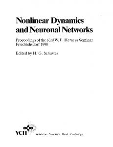
Figure 2. Disorder average maps network with frozen variability in connections to highly symmetric network on the background of fluctuating auxiliary fields Q, which induce additional temporal variability (noise D(Q)) and global variability in connections (µ(Q)).

of fluctuating fields Q Z N (6) hZ[J]i ∼ DQ e− σ2 Q1 Q2 +ln(ZQ [J]) , Z Z T T 1 ˜T ˜ ˜ ˜ eS0 (X,X)+ 2 Q1 X X+Q2 X X+J X . ZQ [J] = DX DX The large dimensional integrals of the free theory ZQ [J] can be solved analytically yielding a two-dimensional interacting theory in the auxiliary fields Q1 and Q2 . The auxiliary field formalism translates the high-dimensional ensemble average over W to a low-dimensional average over Q, i.e. a mapping of the local disorder in the connections to fluctuations of the global connection strength and noise level in a highly symmetric all-to-all connected network, illustrated in Fig. 2 [37]. Only in the special case of vanishing mean connection strength µ = 0, the system factorizes into N unconnected units, each interacting with the same set of fields Q. The all-to-all network not only captures the auto-covariance of a single neuron, but also the cross-covariance with any other neuron. A loopwise expansion [38–40] of the exponent in Eq. (6) around self-consistently determined and sourcedependent saddle points Q∗J of the Q-integrals yields a 1/N expansion of hZ(J)i. For large networks, the zeroth order (tree-level in Q) is sufficient to calculate the twoand four-point correlators that yield the leading order contributions to the mean integral covariances  
D −1 T −1 cij = (1 − µ) = Dr γij (7) 1 − µ 1 − R2 ij and the variance of integral covariances " # 1 1 2 2 2 δcij = R 2 + 1 − R2 Dr χij , (1 − R2 )

(8)

with γij = δij + γ, χij = N1 (1 + δij + O(1/N )), γ = O(1/N ), which depend on the deterministic network √ structure, the spectral radius R = 1 + γ σ of the connectivity matrix W [41], and the noise strength Dr = D + D(Q∗0 ). The latter is renormalized by the strucR2 The tural variability (D(Q∗0 ) = D 1−R 2 , see Fig. 2). average connection strength, however, is not affected

4 (a) auto-covariances 102 101 100

0.0 0.5 1.0 spectral radius R

(b) cross-covariances 102 101 100

0.0 0.5 1.0 spectral radius R

(c)

spectral radius

1.0 0.5 0.0 100 102 104 106 108 network size N

Figure 3. Mean (dark gray) and standard deviation (light gray) of integral auto- (a) and cross-covariances (b) for different spectral radii R. Solid curves indicate analytical predictions, symbols show numerical results for one realization at each parameter setting (dots: Gaussian connectivity; open circles: Erdős-Rényi connectivity; network size N = 1000). (c) Predicted spectral radius of the effective connectivity of the macaque motor cortex network as a function of network size for given moments of experimentally observed parameters of the covariance distribution (Fig. 1, cij = 0.12, δc2ij = 7.89, cii = 16.16, δc2ii = 432.89). The shaded area marks the range of biologically plausible effective network sizes corresponding to the spatial scale of the recordings. The red dashed line indicates the critical point R = 1.

(µ(Q∗0 ) = 0, see Fig. 2). While the previous expressions are obtained from saddle points evaluated at vanishing sources Q∗0 = Q∗J=0 , the distinct dependence of D(Q∗J ) and µ(Q∗J ) on the external sources J reflects fluctuations of auxiliary fields Q across network realizations. These fluctuations in Q1 and Q2 contribute each one term to the dispersion of covariances in Eq. (8) with different scaling in R. This source dependence has been neglected in the pioneering work introducing the functional formulation of disordered systems [39]. The mean connection strength µ determines γ and χij and acts as a negative feedback in inhibitory or inhibition-dominated networks [4]. While this feedback suppresses mean cross-covariances (7), it only yields a subleading contribution to the dispersion (8). The spread of individual cross-covariances is therefore predominantly determined by fluctuations in connection weights. These fluctuations cause broad distributions of cross-covariances of both signs even in a homogeneous network [42]. At a critical point R = 1 (Fig. 3), where the linear system becomes unstable due to the largest eigenvalue of the connectivity matrix W exceeding unity, we observe a divergence of auto- and cross-covariances. In the slightly sub-critical regime, slowly decaying fluctuations generate individual covariances in the network much larger than the average across neurons. The same correlation structure exists in a nonlinear network [12] with infinitesimal additive noise, leading to fluctuating activity also in the regular regime. In this model, the point of linear instability coincides with a transition to chaos and a divergence in topological complexity [43]. The analytic expressions for the moments of covariances Eqs. (7) and (8) can be used to infer network

parameters from experimentally observed covariance distributions. For the highly symmetric network considered here, the application of Wick’s theorem yields at leading order a trivial factor two between the variance of integral auto- and cross-covariances (see definition χij above) and thus requires one free parameter in the inversion of Eqs. (7) and (8). For given network size N , the spectral radius of the effective connectivity W is predominantly determined by the width of the distribution of cross-variances normalized by the mean auto-covariances v u R2 ≈ 1 − u t

1 δc2

.

(9)

1 + N ciiij2

Distributions of covariances can therefore be used to infer the operational regime of the network, i.e. the distance to criticality. Fig. 3c shows that for the distribution of covariances measured in macaque motor cortex (Fig. 1) and biologically plausible network sizes, the linear network model must operate close to criticality to explain the data. The small change of the spectral radius in the biologically relevant range further illustrates the robustness of the result with respect to a potential bias of the experimental estimates due to limited observation time or the number of recorded neurons [5]. Mean integral auto-covariances (7) and the variance of integral cross-covariances (8) are predominantly determined by the global noise level and the spectral radius. Therefore these measures are rather insensitive to specific deterministic features of the connectivity and distributions of noise amplitudes across neurons. This suggests that Eq. (9) also holds qualitatively for more complicated network topologies and variable noise levels. In a biologically plausible Erdős-Rényi network, randomness in connections is controlled by the weight of non-zero connections. Tuning these weights of the effective connectivity by, for example, plasticity mechanisms or external inputs to the network, one can adjust the overall correlation structure and drive the network into a linearly unstable regime with large transients introduced by external perturbations. One can use Eqs. (7) and (8) to uniquely determine the parameters of a homogeneous network of arbitrary size that generates distributions of covariances matching the first two moments of experimental data (Fig. 1). An exception is the variance of integral auto-covariances that is sensitive to the inter-neuron variability of the noise level. A better agreement between the higher-order moments of the experimental distributions for auto- and crosscovariances and the model results requires more realistic network topologies, such as excitatory and inhibitory populations driven by heterogeneous noise and spatially dependent connectivity. We have high hopes that generalizations of the formalism will turn out to be straight forward.

5 We are grateful to Alexa Riehle and Thomas Brochier for providing the experimental data and to Sonja Grün for fruitful discussions on their interpretation. We thank Vahid Rostami for helping us with the analysis of the multi-channel data. The research was carried out within the scope of the International Associated Laboratory “Vision for Action - LIA V4A“ of INT (CNRS, AMU), Marseilles and INM-6, Jülich. This work was partially supported by HGF young investigator’s group VH-NG-1028, Helmholtz portfolio theme SMHB, and EU Grant 604102 (Human Brain Project, HBP).

[1] J. De la Rocha, B. Doiron, E. Shea-Brown, J. Kresimir, and A. Reyes, Nature 448, 802 (2007). [2] E. Shea-Brown, K. Josic, J. de la Rocha, and B. Doiron, Phys. Rev. Lett. 100, 108102 (2008). [3] C. van Vreeswijk and H. Sompolinsky, Science 274, 1724 (1996). [4] T. Tetzlaff, M. Helias, G. Einevoll, and M. Diesmann, PLOS Comput. Biol. 8, e1002596 (2012). [5] A. S. Ecker, P. Berens, G. A. Keliris, M. Bethge, and N. K. Logothetis, Science 327, 584 (2010). [6] M. R. Cohen and A. Kohn, Nat. Rev. Neurosci. 14, 811 (2011), doi:10.1038/nn.2842. [7] A. Renart, J. De La Rocha, P. Bartho, L. Hollender, N. Parga, A. Reyes, and K. D. Harris, Science 327, 587 (2010). [8] M. N. Shadlen and W. T. Newsome, J. Neurosci. 18, 3870 (1998). [9] H. Sompolinsky, H. Yoon, K. Kang, and M. Shamir, Phys. Rev. E 64, 051904 (2001). [10] R. Moreno-Bote, J. Beck, I. Kanitscheider, X. Pitkow, P. Latham, and A. Pouget, Nat. Neurosci. 17, 1410 (2014). [11] I. H. Stevenson and K. P. Kording, Nat. Neurosci. 14, 139 (2011). [12] H. Sompolinsky, A. Crisanti, and H. J. Sommers, Phys. Rev. Lett. 61, 259 (1988). [13] J. P. Crutchfield and K. Young, Phys. Rev. Lett. 63, 105 (1989). [14] T. Toyoizumi and L. F. Abbott, Phys. Rev. E 84, 051908 (2011). [15] L. Molgedey, J. Schuchhardt, and H. Schuster, Phys. Rev. E 69, 3717 (1992). [16] J. Aljadeff, M. Stern, and T. Sharpee, Phys. Rev. Lett. 114, 088101 (2015). [17] J. Kadmon and H. Sompolinsky, Phys. Rev. X 5, 041030 (2015). [18] A. Crisanti and H. Sompolinsky, Phys. Rev. A 36, 4922 (1987). [19] M. Moshe and J. Zinn-Justin, Physics Reports 385, 69 (2003), ISSN 0370-1573. [20] C. De Dominicis and L. Peliti, Phys. Rev. B 18, 353

(1978). [21] N. Brunel, J. Comput. Neurosci. 8, 183 (2000). [22] D. Grytskyy, T. Tetzlaff, M. Diesmann, and M. Helias, Front. Comput. Neurosci. 7, 131 (2013). [23] I. Ginzburg and H. Sompolinsky, Phys. Rev. E 50, 3171 (1994). [24] D. Dahmen, H. Bos, and M. Helias, arXiv (2015), 1512.01073 [q-bio.NC]. [25] V. Pernice, B. Staude, S. Cardanobile, and S. Rotter, PLOS Comput. Biol. 7, e1002059 (2011). [26] J. Trousdale, Y. Hu, E. Shea-Brown, and K. Josic, PLOS Comput. Biol. 8, e1002408 (2012). [27] A. Hawkes, J. R. Statist. Soc. Ser. B 33, 438 (1971). [28] H. Risken, The Fokker-Planck Equation (Springer Verlag Berlin Heidelberg, 1996). [29] A. Riehle, S. Wirtssohn, S. Grün, and T. Brochier, 7, 48 (2013), doi: 10.3389/fncir.2013.00048. [30] P. Martin, E. Siggia, and H. Rose, Phys. Rev. A 8, 423 (1973). [31] C. Chow and M. Buice, The Journal of Mathematical Neuroscience 5 (2015). [32] K. H. Fischer and J. A. Hertz, Spin Glasses (Cambridge University Press, 1991), ISBN 9780511628771. [33] Variability in the determinant can be accounted for perturbatively, but only yields subleading contributions which are suppressed for large network size. [34] H. Nishimori, Statistical Physics of Spin Glasses and Information Processing An Introduction (Calendron Press, Oxford, 2001). [35] C. W. Gardiner, Handbook of Stochastic Methods for Physics, Chemistry and the Natural Sciences (SpringerVerlag, Berlin, 1985), 2nd ed., ISBN 3-540-61634-9, 3540-15607-0. [36] C. Van Vreeswijk and H. Sompolinsky, Neural Comput. 10, 1321 (1998). [37] Note that this follows after integrating over the variables ˜ The result is equivalent to a noise strength D(Q) and X. a connection strength µ(Q) that depend on Q1 and Q2 . [38] H. Sompolinsky and A. Zippelius, Phys. Rev. Lett. 47, 359 (1981). [39] H. Sompolinsky and A. Zippelius, Phys. Rev. B 25, 6860 (1982). [40] J. Zinn-Justin, Quantum field theory and critical phenomena (Clarendon Press, Oxford, 1996). [41] K. Rajan and L. F. Abbott, Phys. Rev. Lett. 97, 188104 (2006). [42] A decomposition of fluctuations into the populationaveraged fluctuation and orthogonal modes yields that the population-averaged fluctuation, which exclusively determines average covariances, is suppressed by the average inhibitory connection weight µ < 0, while the second moment of covariances results from the fluctuations of all remaining modes, which are not suppressed by negative feedback. [43] G. Wainrib and J. Touboul, Phys. Rev. E 110, 118101 (2013).