Distribution of Path Durations in Mobile Ad-Hoc Networks and Path ...

1

Distribution of Path Durations in Mobile Ad-Hoc Networks and Path Selection Richard J. La and Yijie Han

Abstract— We investigate the issue of path selection in multihop wireless networks with the goal of identifying a scheme that can select a path with the largest expected duration. To this end we first study the distribution of path duration. We show that, under a set of mild conditions, when the hop count along a path is large, the distribution of path duration can be well approximated by an exponential distribution even when the distributions of link durations are dependent and heterogeneous. Secondly, we investigate the statistical relation between a path duration and the durations of the links along the path. We prove that the parameter of the exponential distribution, which determines the expected duration of the path, is related to the link durations only through their means and is given by the sum of the inverses of the expected link durations. Based on our analytical results we propose a scheme that can be implemented with existing routing protocols and select the paths with the largest expected durations. We evaluate the performance of the proposed scheme using ns-2 simulation.

I. I NTRODUCTION Multi-hop wireless ad-hoc networks have been the focus of active research in recent years. Unlike a wireline network with a fixed infrastructure, a wireless ad-hoc network can be deployed with no infrastructure and mobile nodes can establish and maintain a network in an autonomous manner. Due to nodes’ mobility, links are expected to be set up and torn down much more frequently than in a wireline network. As a result, a network topology varies with time as the connectivity between nodes changes dynamically. Frequent link failures and network topology changes in mobile ad-hoc networks (MANETs) render the routing protocols designed for wireline networks (e.g., the Internet) rather inefficient. A suite of new routing algorithms have been proposed for MANETs to deal with frequent network topology changes [8], [12], [14], [15]. A detailed discussion of available routing protocols is provided in the monographs [13]. Due to nodes’ mobility, links along a provided path may become unavailable in an unpredictable manner. When one or more links along a path in use become unavailable (which we call a path failure), the path is no longer valid and a path recovery procedure is triggered to find an alternate path. Detecting and recovering from a path failure can take a nonnegligible amount of time (from applications’ viewpoint), during which service to on-going traffic will be disrupted. Such a disruption in service can degrade the performance of time-critical applications. Furthermore, an initiation of path recovery incurs additional overhead. Therefore, from the perspective of providing reliable network service and Authors are with the Department of Electrical & Computer Engineering, University of Maryland, College Park. E-mail: {hyongla,hyijie}@isr.umd.edu.

minimizing control overhead, a good routing algorithm should take into consideration the expected duration as well as other requirements when selecting a path. The duration of a path refers to the amount of time for which the path remains available after its set-up until one of the links along the path fails for the first time. Intuitively the duration of a path should depend on the durations of the links along the path and their dependence structure. Therefore, there is much interest in better understanding the statistical properties of link and path durations and their relation. Better understanding of their statistical properties will allow us to approximate the frequency of disruption in service and resulting overhead. Hence, it will help us evaluate the performance of on-demand routing protocols and the adverse effects of potentially frequent disruptions in service on the performance of upper layers (e.g., Transmission Control Protocol) without having to run time-consuming detailed simulations. A numerical example using the Random Waypoint (RWP) mobility model is given in [5, Section 8]. To the best of authors’ knowledge there is very little known about the distribution of path durations and its relation with those of the links that provide them. Consequently, most of existing routing protocols select a path based on some heuristic argument; the Dynamic Source Routing (DSR) protocol selects the minimum hop path, whereas the Ad-hoc On-demand Distance Vector (AODV) routing protocol selects the first discovered path. Associativity Based Routing (ABR) protocol selects the path with maximum average age of the links. However, it is not clear how the hop count or the average age of the links along a path is related to its (expected) duration. Along this line Sadagopan et al. [17] presented a simulation study of the distribution of multi-hop path durations under various mobility models. Their study shows that the distribution of path duration can be accurately approximated by an exponential distribution when the number of hops is larger than 3 or 4 for all mobility models considered. However, no clear explanation was offered for the emergence of an exponential distribution. In order to correct the current state of affairs Han et al. [5] developed an approximate framework for studying the distributions of path and link durations. They showed that, under certain conditions, the distribution of path duration (under appropriate scaling) converges to an exponential distribution when the number of hops becomes large. This result is in line with the simulation results provided in [17], and is obtained as a simple application of Palm’s Theorem [7, Thm. 5-14, p. 157]. In addition, they explored the connection between the expected duration of a path and the expected durations of the

2

links along the path. To be more precise, they showed that when the number of hops is large, the inverse of the expected duration of a path is approximately given by the sum of the inverses of expected durations of the links along the path. The results reported in [5] provide the first evidence that when the hop count is large, the distribution of path duration can indeed be approximated by an exponential distribution. The application of Palm’s theorem in [5], however, requires that the link excess lives be mutually independent, which is in general not true. The excess life of a link in a path refers to the amount of time the link remains available until it is torn down for the first time after the path set-up. Two neighboring links along a path, for example, share a common node. Clearly, the excess lives of these two neighboring links depend on the mobility of the shared node, introducing some level of dependence in them. Moreover, such local dependence in link excess lives may be more evident under group mobility models where the mobility of a set of nodes may be correlated. Therefore, it is of much interest to see if the same distributional convergence to an exponential distribution holds without the independence assumption and how the parameter of the limit distribution (which decides the expected duration) is affected by the dependence. In this paper we extend the results in [5] by relaxing the independence assumption on the link excess lives imposed in [5]; we only require that the dependence of link excess lives go away asymptotically with increasing hop distance between the links. This assumption can be stated using what is known as a mixing condition (Section V-A). It allows the possibility of relatively strong local dependence in link excess lives which can be exhibited, for example, under group mobility models. We demonstrate that, under some mild conditions (to be stated precisely), the same distributional convergence to an exponential distribution reported in [5] holds under this much weaker condition (Section V-B). We point out that relaxing the independence assumption demands a new technique for proving the distributional convergence and complicates the proof considerably; a suitable extension of Palm’s theorem that deals with dependent processes is not available. We also show that the parameter of the emerging exponential distribution is the same whether the link excess lives are mutually independent or not. In other words, the parameter of the exponential distribution is given by the sum of the inverses of the expected link durations. This suggests that for a path with a sufficiently large hop count the dependence of link excess lives does not significantly affect the path duration distribution. Based on this observation, we outline a scheme that can be implemented in existing routing protocols to select the path with the largest expected duration with minimal communication overhead (Section VI). We implement this scheme in AODV and evaluate the performance gain (Section VII). The paper is organized as follows. A basic framework for modeling path durations is given in Section II. Section III introduces the set-up under which the asymptotic distribution of a path duration with increasing hop count is studied. In Section IV we study a simpler case in which link durations have the same distribution and their dependence is limited to

a finite neighborhood. This is followed by a study of more general cases in which the link duration distributions may be heterogeneous and the dependence is not limited to a finite neighborhood in Section V. We outline how our results can be used to implement a scheme for selecting a path with the largest expected duration during a path discovery phase in Section VI. Simulation results are presented in Section VII to demonstrate the performance gain from our proposed scheme. A word on the notation and convention used throughout: We define all the random variables (rvs) of interest on some common probability space (Ω, F, P). Two IR–valued rvs X and Y are said to be equal in law if they have the same distribution, a fact we denote by X =st Y . The independence between two rvs X and Y is denoted by X ⊥ Y . If G is a probability distribution on IR+ , let m(G) denote its first moment which is always assumed to be finite. Convergence in distribution (with n going to infinity) is denoted byp =⇒ n . For any x in IR2 , with components (x1 , x2 ), set ||x|| = x21 + x22 .

II. A BASIC F RAMEWORK This section describes the same basic framework that we borrow from [5] for our analysis: Consider a MANET where a set of nodes creates and maintains network connectivity. We assume that an on-demand algorithm is used and a path between a source node and a destination node is set up only when a request is made. Let V = {1, . . . , N } denote the set of N mobile communicating nodes. Each node moves across a domain D of R2 or R3 according to some mobility model. Due to nodes’ mobility, links between nodes are set up and torn down dynamically. We assume that a link between two nodes is either up or down. Two nodes without a link between them establish such a link as soon as they become reachable, e.g., when they come within a transmission range of each other or when the signal to interference and noise ratio (SINR) at the receiver exceeds certain threshold, and packets from each other can be successfully decoded. The latter case captures the characteristics of the physical layer (e.g., path loss and channel fading) more accurately. Although this is not needed for the analysis, communication links are assumed bidirectional since such bidirectional communication is typically required between two nodes for reliable forwarding of packets, for instance, by means of acknowledgments for each transmission. Establishing a path from a source node to a destination node requires simultaneous availability of a number of communication links that are up at the time of path request and collectively provide the desired connectivity between the source and the destination. The duration of a path provided by the underlying routing protocol is then defined as the amount of time that elapses until one of the links along the path goes down for the first time after the path set-up. A link may go down (which we call a link failure) due to either mobility or degradation in channel condition. For simplicity of analysis, path set-up delays are assumed negligible. A. Reachability processes We model the situation outlined above as follows: For a pair of distinct nodes i and j in V , we introduce a {0, 1}-valued

3

reachability process {ξij (t), t ≥ 0} with the interpretation that ξij (t) = 1 (resp. ξij (t) = 0) if the unidirectional link from node i to node j, denoted by “link” (i, j), is up (resp. down) at time t ≥ 0. Since the communication links are assumed bidirectional, we must have ξij (t) = ξji (t). The process {ξij (t), t ≥ 0} is simply an alternating on-off process, with successive up and down time durations given by the rvs {Uij (k), k = 1, 2, . . .} and {Dij (k), k = 1, 2, . . .}, respectively. The reachability processes can be defined in a number of ways. For example, for each i in V , let {X i (t), t ≥ 0} describe the trajectory of node i, i.e., X i (t) denotes the position of node i at time t ≥ 0. If we do not explicitly model channel fading between nodes, it is reasonable to assume that two nodes can communicate with each other reliably if the distance between them is smaller than some fixed transmission range rmin > 0. Hence, a link between two distinct nodes i and j in V exists at time t ≥ 0 if and only if their distance is smaller than rmin , leading to the definition ξij (t) := 1 [||X i (t) − X j (t)|| ≤ rmin ] ,

t ≥ 0.

(1)

Alternative models can take into account the physical layer characteristics of the channel. For instance, two nodes i and j in V can maintain a link between them at time t ≥ 0 if and only if   Pj · Fji (t) Pi · Fij (t) , min >Γ (2) Ψi (t) Ψj (t) for some threshold Γ > 0, where Pi is the maximum transmission power of node i, and F (t) = (Fij (t)) denotes the channel gain matrix (including fading) at time t with F ji (t) ≥ 0 and Fii (t) = 0, i, j = 1, . . . N . Different choices of Ψi (t) in (2) lead to different physical layer models. In the simplest form, one can assume that a node i can decode the packets from node j if and only if the received signal power exceeds some threshold Γ > 0 [2], [16]. In this case the reachability process between nodes i and j is given by (2) with Ψi (t) = 1 as the numerators give the largest achievable received signal power at the nodes. Similarly, if one assumes that packets can be successfully decoded if and only if the achieved SINR exceeds the threshold Γ [3], [4], then the reachability process between nodes i and j is again given by (2) with X Ψi (t) = Wi + Pk (t) · Fki (t) , (3) k∈T X(t)\{j}

where Wi is the noise variance at node i, T X(t) is the set of transmitters at time t and Pk (t) denotes the transmission power of node k. The right hand side of (3) represents the sum of noise power and interference at node i at time t. This implies that nodes i and j have connectivity if and only if the achieved SINR value using the maximum transmission power exceeds Γ in both directions.

the relation E(t) := {(i, j) ∈ V × V : ξij (t) = 1},

(4)

where by convention we set ξii (t) = 0 for each i in V and all t ≥ 0. Thus, a path can be established (in principle) between nodes s and d at time t ≥ 0, if node d is reachable from node s by a path in the undirected graph derived from the directed graph (V, E(t)). Let Psd (t) ⊆ 2E(t) denote the set of paths from node s to node d providing this reachability. This set of paths is empty when the nodes s and d are not reachable from each other at time t. When non-empty, this set Psd (t) may contain more than one path since multiple paths may exist between nodes s and d. In such a case, the routing protocol in use selects one of the paths in Psd (t) and let Lsd (t) denote the set of links in the selected path. For each link ` in Lsd (t), let T` (t) denote the time-to-live or excess life after time t, i.e., T` (t) is the amount of the time that elapses from time t onward until link ` is down. The time-to-live or duration Zsd (t) of the established path from node s to node d using the links in Lsd (t) is defined as the amount of time that elapses from time t until one of the links in Lsd (t) goes down, at which point a path recovery procedure is initiated. This quantity is simply given by Zsd (t) := min (T` (t) : ` ∈ Lsd (t)) ,

t ≥ 0.

(5)

III. T HE S ET- UP AND M ODELING A SSUMPTIONS In this paper we are interested in studying the distribution of path duration as the number of hops becomes large. In the following subsection we first describe the set-up used to model this scenario. Then, we state the modeling assumptions under which the distributional convergence of path duration is established with increasing hop count. A. The set-up In order to study the distribution of path duration with a large hop count, we investigate the asymptotic distribution of path duration (under appropriate scaling of link excess lives) as the number of hop count increases. This is done by introducing a parametric scenario with a sequence of networks in which both the number of communicating nodes and the domain across which they travel increase: For each n = 1, 2, . . ., let V (n) = {1, . . . , N (n) } and D(n) denote the set of mobile nodes and the domain across which the nodes move, respectively. For each node i in V (n) , the (n) D(n) -valued process {X i (t), t ≥ 0} denotes the trajectory of node i in D(n) . The stochastic process that governs the arrival of path requests is assumed to be independent of these trajectory processes. 1. Scaling – We are interested in the situation where N (n) ∼ nN (1)

and

Area(D(n) ) ∼ n · Area(D(1) )

(6)

as n goes to infinity;1 it is customary to reparameterize so that N (n) = n. When in force, the scaling (6) guarantees N (n) N (1) ∼ , Area(D(n) ) Area(D(1) )

B. Path duration Next we endow V with a time-varying graph structure by introducing a time-varying set E(t) of directed edges through

t≥0

1 From

now on we omit this qualifier in all asymptotic equivalences.

4

so that the density of nodes, i.e., the number of nodes per unit area, is asymptotically constant. 2. Stationarity – As the system is expected to run for a long time, we can assume that steady state has been reached. This possibility is captured by taking the N (n) trajectory processes to be jointly stationary. Joint stationarity of the trajectory (n) (n) −1) reachability processes also implies that the N ×(N 2 processes are jointly stationary. For distinct i < j in V (n) , (n) (n) let the rvs {(Uij (k), Dij (k)), k = 1, 2, . . .} denote the sequence of up and down times for the reachability process (n) {ξij (t), t ≥ 0}. Writing   (n) (n) W (n) (k) = (Uij (k), Dij (k)), i < j, i, j ∈ V (n) ,

k = 1, 2, . . ., we require that the sequence of rvs {W (n) (k), k = 2, 3, . . .} be strictly stationary. In partic(n) ular, for distinct i < j in V (n) , the sequence {(Uij (k), (n) Dij (k)), k = 2, 3, . . .} constitutes a stationary sequence (n) (n) (n) with generic marginals (Uij , Dij ). We denote by Gij the (n) cumulative distribution function (CDF) of U ij . This model is general enough that link dynamics due to both mobility and channel fading can be captured by a suitable choice of the (n) CDFs for Uij . Well-known results for renewal processes and independent on-off processes in equilibrium [7, Sections 5-6] can be generalized as follows: With ` = (i, j), in the notation introduced in Section II, we have i h (n) (n) (n) (7) P T` (0) ≤ x ξij (0) = 1 = F` (x), x ∈ R (n)

where the conditional probability F` (x) is given by  ( Rx (n) 1 (y) dy if x > 0 1 − G (n) (n) ` m(G` ) 0 (8) F` = 0 if x ≤ 0 (n)

for some link duration CDF G` with support in IR+ . In (n) other words, F` is simply the distribution of the forward (n) recurrence time associated with U` . From (8) it is easy to see that the duration of a one-hop path has a non-increasing (n) probability density function (PDF). If X` denotes any R+ (n) valued rv distributed according to F` , then the relation (7) simply states, with a little abuse of notation, that i h (n) (n) (n) T` (0) ≤ x ξij (0) = 1 =st X` . The rv (5) can now be viewed as the rv Z (n) defined by   (n) (9) Z (n) := min X` : ` = 1, . . . , H (n) (n)

where H (n) = |Lsd (0)|. Due to the underlying stationarity assumptions, it clearly suffices to consider only the case t = 0 as we do from now on.

depends on the reachability processes at t = 0. Second, the reachability processes are usually not mutually independent. This is clear from either formulation (1) or (2). In this subsection we explain how we handle these issues. (n)

1. Asymptotics of the random set Lsd (0) – With increasing network size under scaling (6) the average number of hops in a path between two randomly selected nodes is expected to increase with n. For example, consider the model with a fixed domain, in which the connectivity between two nodes is determined by (1).2 We first select the locations of a source and a destination according to some stationary spatial distribution of the nodes. Then, for each n = 3, 4, . . ., place the remaining n − 2 other nodes on the domain according to the same stationary distribution √ while decreasing the transmission range of the nodes as 1/ n. If minimum hop routing is employed, the number of √ hops along the shortest path will increase approximately as n. Thus, we assume that a pair of nodes s and (n) d in V (n) can be selected such that limn→∞ |Lsd (0)| = ∞, (n) where for convenience the sequence {|Lsd (0)|, n = 1, 2, . . .} is assumed to be deterministic. 2. Dependence of the reachability processes and link excess (n) lives – As mentioned earlier, the link excess lives {X ` , ` = 1, . . . , H (n) } in (9) are not mutually independent in general. The authors of [5] skirted this difficulty by assuming that the reachability processes {ξij (t), t ≥ 0} are mutually (n) independent so that the rvs {X` , ` = 1, . . . , H (n) } are mutually independent. They provided a simulation study (Section 9 in [5]) using the RWP mobility model without pause to justify this assumption; it shows that the correlation coefficient of link excess lives in (9) decays rapidly with increasing hop distance between the links. More specifically, it indicates that the correlation coefficient of link excess lives between two neighboring links is small and that of two links separated by intermediate link(s) is almost negligible. This observation provides some evidence that the dependence of link excess lives may indeed decrease quickly with hop distance in some cases. However, the observed fast decrease of correlation in hop distance may be a consequence of the fact that the mobility of a node in the RWP model is independent of other nodes, and if the mobility of a set of nodes is strongly correlated (e.g., soldiers in a platoon partaking in a mission), this may no longer be true. In the following sections we relax the independence assumption of the reachability processes in [5] and replace it with what are commonly known as mixing conditions. These conditions impose a form of asymptotic independence as the hop distance between links increases, while allowing dependence in an (unbounded) neighborhood. IV. F INITE D EPENDENCE WITH H OMOGENEOUS L INK D URATION D ISTRIBUTION

B. Modeling assumptions

In this section we consider a simpler case where link durations have the same CDF G with support in IR + and the dependence in link excess lives is limited to a finite local

There are a few sources of difficulty in modeling and studying the distribution of path durations: First, the set L sd (0) of links in the selected path is a random subset of E(0), which

2 Decreasing the transmission range while keeping the domain fixed has the same effect as increasing the domain size while keeping the transmission range fixed.

5

neighborhood. First, in order to model the link excess lives, we introduce a stationary sequence of rvs {X i , i = 1, 2, . . .} whose CDF is given by  1 Rx m(G) 0 (1 − G(y)) dy , if x > 0 . (10) F (x) = 0, if x ≤ 0 (n)

We let X` = X` for all n ∈ + := {1, 2, . . .} and all ` ≤ H(n), i.e., rv X` is used to model the excess life of the `th link in an H(n)-hop path. The path duration of an H(n)-hop (n) path is modeled by rv Z (n) := min(X` : ` = 1, . . . , H(n)). The rvs Xi , i = 1, 2, . . ., are identically distributed from the stationarity assumption, but may not be mutually independent. The aforementioned assumption of finite dependence of link excess lives is given by the following: Assumption 1: (m-dependence [18]) The rvs Xi , i = 1, 2, . . ., satisfy X` ⊥ X`0 if |` − `0 | > m, where m is a finite positive integer. This assumption is consistent with the findings in [5, Fig. 9], where the dependence in link excess lives under the RWP mobility model appears to be limited to a very small neighborhood. Assumption 2: For every x ≥ 0 and any given  > 0, there exists an integer n? = n? (x; ) such that x ≤, n = n? , n? + 1, . . . G n Assumption 2 is equivalent to saying that a link duration is strictly positive with probability one, i.e., lim n→∞ G(x/n) = G(0) = 0. It is obvious that this assumption holds trivially if the CDF G is continuous (i.e., link durations can be modeled as continuous rvs). Therefore, it is a reasonable assumption. Theorem 1: Suppose that Assumptions 1 and 2 hold for the stationary sequence {Xi , i = 1, 2, . . .} and the CDF G. If the condition 1 lim max P [Xi < c, Xj < c] c↓0 P [Xi < c] |i−j|≤m = lim max P [Xj < c | Xi < c] (11) c↓0 |i−j|≤m

=0

holds, then h i  1 − e−λx , (n) lim P H(n) · Z ≤x = 0, n→∞

if x > 0 (12) if x ≤ 0

where λ = (m(G))−1 . Proof: A proof is provided in Appendix III of the supplemental document due to a space constraint.

Theorem 1 tells us that as the number of hops H(n) along a path increases the distribution of path duration can be well approximated by an exponential distribution with parameter H(n) · λ for all sufficiently large H(n). Note that (n) rv Z (n) = min(X` : ` = 1, . . . , H(n)) tends to decrease with increasing H(n). This is also obvious from the fact that H(n) · λ → ∞ as n → ∞. Thus, in order to keep Z (n) from converging to a constant rv with value zero as H(n) increases, rv Z (n) is scaled by the hop count H(n) in (12).

It is interesting to note that the parameter of the emerging exponential distribution is given by the same λ = 1/m(G) whether the rvs {Xi , i = 1, 2, . . .} are assumed to be locally dependent as here or mutually independent as assumed in [5]. The condition in (11) implies that as c ↓ 0, the rare events {Xj < c} do not occur in clusters in a local neighborhood of node i. One interpretation of this condition is as follows: Assume a very small c. Rare events of link excess lives being smaller than c are primarily caused by nodes being close to the edge of their transmission ranges and about to move out of the transmission ranges at the time of path set-up (rather than one or both of the nodes moving at an extremely high speed). Condition (11) implies that one pair of neighboring nodes being about to leave the transmission range of each other at the time of path set-up, does not mean the same is true for other pairs of neighboring nodes along a path, which is reasonable. This condition is validated in the case of the RWP mobility model in Appendix V of the supplemental document. V. G ENERAL D EPENDENCE WITH H ETEROGENEOUS L INK D URATION D ISTRIBUTIONS In the previous section we considered the simpler case where the dependence in link excess lives is limited to a finite neighborhood. As mentioned earlier, this may be reasonable in some cases. However, we show that it can be relaxed considerably. To be precise, the same distributional convergence can be obtained even when the dependence of link excess lives is not bounded to any finite neighborhood and the link duration distributions are heterogeneous. In this section we first define the mixing conditions that describe the manner in which the dependence of link excess lives decays with the hop distance between the links. Then, we establish the distributional convergence of path duration in more general cases under the mixing conditions. A. Mixing conditions (n)

Suppose that W := {Wi , n = 1, 2, . . . ; i = 1, . . . , h(n)} is an array of IR-valued rvs, where {h(n), n ≥ 1} is a sequence of positive integers with limn→∞ h(n) = ∞. Denote the (n) (n) (n) (n) joint CDF of rvs {Wi1 , Wi2 , . . . , Win } by Ji1 ···in . For (n) (n) notational simplicity we write Ji1 ···in (u) for Ji1 ···in (u, . . . , u). Let {un , n ≥ 1} be a sequence of real numbers (which typically increases with n) and A := {αn,m , n = 1, 2, . . . ; m = 1, . . . , h(n)} be an array of non-negative real numbers such that, for any integers 1 < i1 < · · · < ip < j1 < · · · < jq ≤ h(n) where j1 − ip > m, we have (n) (n) (n) Ji1 ...ip j1 ...jq (un ) − Ji1 ...ip (un )Jj1 ...jq (un ) ≤ αn,m . (13)

Definition 1: (D(un ) condition [10], [11]) Suppose that we can find a sequence {m(n), n = 1, 2, . . .} of non-negative integers and an array A of real numbers satisfying the condition in (13) such that (i) limn→∞ m(n) = ∞, (ii) m(n) = o(h(n)), i.e., limn→∞ m(n) lim αn,m(n) = 0. Then, we h(n) = 0, and (iii) n→∞ say that the array W satisfies the condition D(u n ).

6

The condition D(un ) imposes a form of “dependence de(n) cay”: As n increases, the dependence of two events {W i1 ≤ (n) (n) (n) un , . . . , Wip ≤ un } and {Wj1 ≤ un , . . . , Wjq ≤ un } decreases as the distance j1 − ip between the two sets of rvs increases. However, since m(n) → ∞, it allows dependence in an unbounded neighborhood. One can easily verify that a sequence that satisfies the m-dependence condition in Assumption 1 satisfies the condition D(un ) with any sequence {un , n ≥ 1}. In order to state the definition of the second mixing condition, we first need to introduce some notation. Let k be a fixed positive integer. We divide the interval {1, 2, . . . , h(n)} into k + 1 disjoint subintervals3 : The first k subintervals have a length n0 := bh(n)/kc, where bxc denotes the integer part of x, and the last interval has a length smaller than k. For j = 1, 2, . . . , k, define (n)

Ik,j = {(j − 1) · n0 + 1, . . . , j · n0 } , and (n)

Ik,k+1 = {k · n0 + 1, . . . , h(n)} . (n) |Ik,j |

= n0 for j = 1, . . . , k, and 0 ≤ Note that where |I| denotes the cardinality of I.

(n) |Ik,k+1 |

< k,

Definition 2: The array W is said to satisfy the condition D0 (un ) if, for all j = 1, 2, . . .,   i  h X 1 (n) (n) =o lim P W i > u n , W i0 > u n n→∞ k (n) i,i0 ∈Ik,j :i j .

(14)

A sufficient condition for the condition D 0 (un ) to hold is h i  h(n) 2 (n) (n) c · sup P W i > u n , W i0 > u n b n→∞ k (n) i,i0 ∈Ik,j :i j . (15) k lim

The interpretation of the condition D 0 (un ) in the context of our problem will be provided shortly. B. Distributional convergence (n)

(n)

Define W` = (X` )−1 , ` = 1, . . . , H(n). Let W := (n) {W` , n = 1, 2, . . . ; ` = 1, . . . , H(n)}. We denote the (n) (n) CDF of rv W` by J` . We first make the following two assumptions. They are the same assumptions imposed in [5, Assumptions 1 and 2] for independent link excess lives cases. Assumption 3: For every x ≥ 0,4    x (n) =0. lim max G` n→∞ `=1,...,H (n) H(n) 3 We call a finite set of consecutive integers {i , . . . , i } an interval with 1 2 length i2 − i1 + 1. 4 In [5] the rvs X (n) are implicitly scaled by H(n), while in this paper ` this scaling is carried out explicitly.

A more concrete way to express Assumption 3 is as follows: For every x ≥ 0 and any given  > 0, there exists an integer n? = n? (x; ) such that   x (n) max G` ≤ , n = n? , n? + 1, . . . H(n) `=1,...,H (n) It is clear that the interpretation of this assumption is the same as that of Assumption 2 and states that a link duration is strictly positive with probability one.   (n)

(n)

Assumption 4: (scaling) Let λ` = m(G` ) exists some positive constant λ such that H(n) 1 X (n) λ` = λ . n→∞ H(n)

lim

−1

. There

(16)

`=1

Assumption 4 simply means that the link excess lives are scaled (by the average of the inverses of expected link durations divided by λ) so that we can define the parameter of the limit distribution. Under Assumption 3, one can show that Assumption 4 is equivalent to the following assumption. Assumption 4A: There exists some positive constant λ such that, for any fixed x ∈ (0, ∞), we have  H(n) X  (n) H(n) P W` > →λ·x as n → ∞ . x `=1

Lemma 1: Suppose that Assumption 3 holds. Let x be some positive real number and un = H(n)/x, n = 1, 2, . . .. Then, for any sequence {m(n), n = 1, 2, . . .} that satisfies conditions (i) - (ii) of Definition 1, we can find an array A of real numbers which satisfies (13) and condition (iii) in Definition 1. Proof: A proof is provided in Appendix IV of the supplemental document due to lack of space. Lemma 1 implies that, under Assumption 3, the array W = (n) {W` , n = 1, 2, . . . ; ` = 1, . . . , H(n)} always satisfies the condition D(un = H(n)/x) for any x in (0, ∞). In fact, in the proof we prove a slightly stronger result: For any integers 1 < (n) i1 < · · · < ip < j1 < · · · < jq ≤ H(n), the events {Wi1 ≤ (n) (n) (n) H(n) ≤ H(n) ≤ H(n) x , . . . , W ip x } and {Wj1 x , . . . , W jp ≤ H(n) } become asymptotically independent as n increases. In x (n) (n) (n) other words, |Ji1 ...ip j1 ...jq (un )−Ji1 ...ip (un )Jj1 ...jq (un )| → 0. For the cases with dependent link excess lives, we introduce two additional assumptions. Assumption 5: For any sequence {Iˆ(n) , n = 1, 2, . . .} of sets of consecutive positive integers, where Iˆ(n) ⊂ {1, . . . , H(n)}, ! X (n) 1 |Iˆ(n) | λ` = O . H(n) H(n) (n) `∈Iˆ

A sufficient condition for Assumption 5 to hold is that there exists some arbitrarily small positive constant ε such (n) that the expected link durations satisfy m(G ` ) ≥ ε for all n = 1, 2, . . . and ` = 1, . . . , H(n). The interpretation of this assumption is that the expected link durations do not

7

decrease to zero with increasing network size. Since the link durations are likely to depend on the nodes’ mobility and their transmission ranges but not directly on the network size, this is a reasonable assumption. (n)

Assumption 6: The array W = {W` , n = 1, 2, . . . ; ` = 1, . . . , H(n)} satisfies the condition D 0 (un ) with un = H(n) x for any x ∈ (0, ∞).   The condition D 0 un = H(n) implies that the rare events x n o (n) x Xj ≤ H(n) in a neighborhood are not strongly correlated x → 0). The role and interpretation of as n → ∞ (hence H(n) this condition are similar to those of condition (11) in the mdependence case (stated at the end of Section IV). Theorem 2: Suppose that Assumptions 3 - 6 hold. Then, we have h i  1 − e−λx , if x > 0 (n) lim P H(n) · Z ≤x = (17) 0, if x ≤ 0 n→∞ Proof: The proof is given in Appendix I.

Theorem 2 states that the distribution of an h-hop path can be well approximated by an exponential distribution for all sufficiently large h. As a byproduct it also tells us that if the link duration distributions are given by G ` , ` = 1, . . . , h, the P expected duration of the path can be approximated by −1 1/( `=1,...,h (m(G` )) ). Somewhat surprisingly, the parameter of the emerging exponential distribution in (17) is the same as that of the exponential distribution with independent link excess lives [5, Theorem 2]. This holds even with somewhat strong local dependence that may exist, and is consistent with the similar observation made in Section IV. This again suggests that the distribution of path duration is not significantly affected by the dependence of the reachability processes and link excess lives when the hop count is sufficiently large. VI. A N OUTLINE OF A PROPOSED SCHEME Detecting a link failure and finding an alternative path can take a non-negligible amount of time in practice. This is because link failures are often detected through a failure to receive/exchange a control message over a pre-determined period. When local recovery is unsuccessful after a link failure, packets queued at the originator of the failed link and additional packets on the way to the node which were to be routed using the link, will eventually be dropped by the node and must be retransmitted by their senders. These dropped packets lead to a waste of wireless resources. Moreover, losses of consecutive packets cause the transport layer protocol to back off, reducing its transmission rate. This may cause senders to rely on timeout to detect the packet losses, which can take more than a few seconds. Hence, frequent link failures along the paths in use will result in disruptions in service and degrade the performance of applications, especially that of time critical applications. For these reasons a routing algorithm should consider its expected duration in addition to other qualities (e.g., estimated available bandwidth or congestion level) when choosing a path . In a large scale MANET the hop distance between a source and a destination is likely to be large [4]. Our results in the

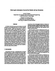
previous sections tell us that when hop counts are large, (i) the distribution of path duration can be well approximated by an exponential distribution and (ii) the inverse of the expected duration of a path is approximately given by the sum of the inverses of the expected durations of the links along the path. Thus, in order to approximate the expected duration of a path, a source needs to know only the sum of the inverses of the expected link durations. Unfortunately, accurate estimation of the expected link durations along a path is difficult in practice. Instead, we approximate them using average link durations experienced by the nodes: Under our scheme each node maintains the average duration of the links that it establishes with other nodes. These average link durations are used as estimates to the expected link durations along a path and are provided to the source during a path discovery phase. Suppose that a node has routing information for a requested destination. Then, it generates a reply message and specifies the inverse of its estimate of the expected duration of the path to the destination in a field Inverse Path Duration (IPD) in the reply. A node that receives a reply message, first adds to the IPD value the inverse of its average of link durations, and then forwards it to the next upstream node. Finally, when the source receives the reply message, it adds the inverse of its average link duration to the IPD value. Then, the source chooses a path with the smallest IPD value, i.e., the largest estimated expected duration. Path Request

Path Request

λ (n2) + λ (n1) + λ (S) Fig. 1.

n1

S

n2

Reply

Reply

λ (n2) + λ (n1)

λ (n2)

D

An example of an estimation of expected path duration.

Let us explain this procedure using the example shown in Fig. 1. The source node S wants to find a path to destination node D and broadcasts a path request to its neighbors. Assume that node n1 does not have routing information for D and forwards the request to its neighbor, node n2. Assume that node n2 has routing information for D. It generates a reply with the initial IPD value of λ(n2) , which is the inverse of its average link duration. Here node n2’s average link duration is used as an estimate of the expected duration of its link with D. Then, it forwards the reply to node n1. Upon receiving the reply, node n1 adds the inverse λ(n1) of its average link duration to the IPD value and forwards the reply to source node S. Again, node n1’s average link duration is used in place of the expected duration of its link with n2. When S receives the reply, it first adds λ(S) to the IPD value of λ(n2) + λ(n1) in the reply. Then, it uses the inverse of the final IPD value as an estimate of the expected duration of the discovered path {(S, n1), (n1, n2), (n2, D)}. As only the sum of the inverses of average link durations is collected, this proposed modification can be easily implemented in available on-demand routing algorithms with minimal overhead. It is also possible with our scheme that a node classifies its neighbors and maintains a separate average link duration for

8

each type of neighbors. The reason for maintaining separate averages is as follows. A large scale MANET is likely to comprise many different types of nodes. For example, a Future Combat System (FCS) will include different types of vehicles (e.g., jeeps, tanks, etc.), soldiers, and possibly aerial vehicles. Clearly, the duration of a link between two nodes will depend on their mobility and communication capabilities. Thus, the durations of links a node establishes with its neighbors over time will be dependent on their mobility and communication capabilities, as well as its own. By maintaining separate averages, we can improve the accuracy of the estimates of expected link durations. This is demonstrated using ns-2 simulation results in Section VII.

hop counts. To be more precise, when more than one path to a destination are discovered, the paths are first ranked by decreasing destination sequence number. If two or more paths have the same sequence number, then the one with a smaller IPD value takes a higher preference as it has a larger estimated expected duration than the others. Finally, if the first two are the same, the path with a smaller hop count is preferred. This is shown in Fig. 2. The path with the highest preference is used as the primary path for routing packets when needed. Before ranking Dest Seq. #

IPD value

hop count

Dest Seq. #

IPD value

hop count

143

13

4

144

15

3

144

17

2

144

17

2

144

15

3

143

13

2

143

13

2

143

13

4

A. Implementation in AODV We implemented our proposed scheme in the AODV routing protocol to evaluate the potential gain in path durations. Most of our changes are limited to the path request and reply messages and their handling. The rest of the AODV scheme is left intact. Since our primary interest is to study the potential benefits of the path selection scheme (rather than proposing a complete routing protocol), we did not attempt to minimize the overhead it generates. Such overhead is likely to depend on the routing protocol in which the proposed scheme is implemented, and the overall overhead of the integrated routing protocol should be minimized. Each node maintains two separate counters - a sequence number and a broadcast ID. The sequence number is incremented when (i) the node generates a new path request message or (ii) it is the requested destination in a path request message and generates a path reply message. This sequence number is used to indicate the freshness of the path request or reply message. Every node also keeps an average of the link durations it experienced in the past. As mentioned earlier, a node can maintain a separate average for each type of neighbors by classifying them. Route entry – A node creates and maintains a route entry for each known destination node.5 However, unlike in AODV, the node can keep up to kp paths (instead of a single path), where kp is a design parameter. In our simulation the value of k p is set to three. The information of each path is recorded in a subentry with four fields: (i) destination sequence number, (ii) next hop to the destination, (iii) hop count, and (iv) Inverse Path Duration (IPD). The IPD field contains the the sum of the inverses of expected link durations approximated using average link durations and reported in a path reply message during path discovery. In order to avoid keeping redundant path information we require that the next hop to the destination of these paths be different. If there is more than one path available, one of them is selected as the primary path as follows. The others are used as backup paths in case the primary path fails. Ranking route subentries – The paths in a route entry are ranked first based on the destination sequence numbers, and then based on the IPD values. Ties are broken using the 5 The routing protocol running at a node may not be aware of node’s neighbors at the beginning when the route entries are empty.

After ranking

Fig. 2.

Ranking of discovered paths.

Path or route request – When a source does not have routing information for a desired destination, it initiates a path discovery process; it first increments its sequence number and broadcasts a path request message to its neighbors. A path request message contains (i) source ID and its sequence number, (ii) source broadcast ID, (iii) destination ID and its sequence number, and (iv) hop count to the source. The hop count is initially set to one. Each path request message is distinguished by its source ID and broadcast ID. When a node receives a path request message, it carries out the following: 1) It checks if there is a subentry for the source in which the next hop is the neighbor that forwarded the request message. If there is no such subentry, it creates a subentry using the information contained in the request message. The IPD value is set to infinity, indicating the information is not available, because the request message does not contain an IPD value. If there is such a subentry and the sequence number in the request message is larger than the one in the subentry, it updates the source sequence number and the hop count. After the update, it re-ranks the paths to the source based on the new sequence number and the hop count. 2) If the node had received another copy of the same request message, it terminates the message. Otherwise, if it is not the requested destination node in the message and has no routing information to the destination, it increases the hop count in the message and rebroadcasts the message to its neighbors. Path or route reply – If an intermediate node has a route entry for the destination with the destination sequence number no smaller than the destination sequence number in the request message, it generates a path reply message. The reply message contains (i) destination ID and its sequence number, (ii) IPD value, and (iii) hop count. For the destination sequence number, IPD value, and hop count, the information in the subentry for the primary path to the destination node is used. The reply message is then sent to the neighbor node that forwarded the request message, and the request message is terminated. If a copy of the path request message reaches the destination node, the destination generates a reply message. It first increases its sequence number to the maximum of its current

9

sequence number and the destination sequence number in the request message. Then, it generates a reply message with the same three fields in the reply message generated by an intermediate node. The initial value of the IPD and the hop count are set to zero. If the destination node receives multiple copies of the same path request message from different neighbor nodes, it can generate more than one reply message. When an intermediate node receives a reply message, it first adds the inverse of its average link duration to the IPD value in the reply message. Recall that the node may classify the neighbor that forwarded the reply message and add the average link duration corresponding to the neighbor’s type when a separate average is kept for each type of neighbors. After incrementing the IPD value, the intermediate node updates its routing information to the destination: It creates a temporary subentry for the newly discovered path to the destination with the information provided in the reply message. Then, it checks if the new path is better than the kp -th ranked path in the entry for the destination. If it is, then it re-ranks the paths, including the newly discovered path, and inserts the new subentry in the route entry for the destination. Otherwise, it discards the temporary subentry. If the reply message is the first reply the node receives for the corresponding request, then it forwards the reply to its upstream neighbor(s). Here we allow the node to forward the reply to up to kr (≤ kp ) neighbors that relayed a copy of the request message to the node. This is done to increase the number of discovered paths (than in AODV) so that the source can choose the best path among them. These kr upstream nodes are selected based on their ranking. The parameter k r may be adapted based on the average degree of the nodes. 6 In our simulation kr is set to three. If the reply message is not the first reply, but the new path has a smaller IPD value than the previous primary path to the destination, then the node can still forward the reply message. This is to advertise the discovery of a more reliable path, i.e., a path with a larger expected duration. However, we did not use this feature in the simulation, and only the first reply is forwarded. Finally, when the source receives a reply message, it first updates the hop count and the IPD value using its average link duration and then its route entry for the destination. Data transmission can begin after the first path to the destination is discovered. However, after processing a newly arrived reply message, the source may switch its primary path to the destination if the newly discovered path has a smaller IPD value than the previous primary path. When a link failure occurs, the node that detects the failure first attempts a local recovery if there is a cached backup path in the route entry for the destination. The details of our local recovery scheme are described in [6] and are omitted in this paper. If the local recovery fails, it broadcasts a “route error” message. The error message contains a list of destination nodes affected by the link failure. Each node that receives an error message checks if any of the paths in its route entries traverses the failed link. If there is any such path, the corresponding 6 When the average degree is large, even a small value of k will allow the r source to discover multiple available paths to choose from. If the network is sparsely connected, then a larger value of kr may be preferred.

subentry is removed. If a primary path is affected, it initiates a path recovery procedure when necessary. VII. S IMULATION RESULTS In this section we evaluate the performance gain (in path duration) from our scheme outlined in the previous section. The simulation is run with 200 nodes moving in a 2 km × 2 km rectangular region. The RWP mobility model is employed. The transmission range of the nodes is set to 250 m. There are two classes of nodes; the speed of a class 1 and class 2 node is uniformly distributed in [1, 5] m/s and [10, 30] m/s, respectively. The reason for having two classes of nodes with different speed ranges is to create a scenario with heterogeneous nodes that experience diverse link durations in the field (e.g., soldiers vs. tanks or jeeps). Slower moving class 1 nodes in general experience longer link durations than faster moving class 2 nodes in our simulation due to the same fixed transmission range. Speeds of the nodes are chosen independently of the selected waypoints and previous speeds. Each run of simulation is for 1,200 seconds, and a total of 126 runs are carried out with different random seeds. 7 However, in order to reduce the effects of transient period data are collected only in the last 800 seconds of each run. A total of approximately 5,000 connections are set up between randomly selected source and destination nodes. The interarrival times of connection requests are given by independent and identically distributed rvs, each of which is a sum of 5 seconds and an exponential rv with a mean 15 seconds. Each connection request generates a path request message, triggering a path discovery phase. Therefore, in the last 800 seconds of each run we generate on the average 40 path request messages. We simulate three different scenarios by varying the number of class 1 nodes (hence class 2 nodes as well) to illustrate the benefits of our scheme and a trend that emerges. We first begin with 140 class 1 nodes and increase it to 160 and then to 180. Our scheme is run under two different modes: In the first mode, each node maintains a single average link duration for all neighbor nodes. In the second mode each node classifies the neighbors and maintains two separate averages - one for class 1 neighbors and the other for class 2 neighbors. The CDFs of link duration under our scheme for the 160 vs. 40 scenario are shown in Fig. 3. In the first mode, we plot the distributions seen by class 1 nodes and class 2 nodes. In the second mode, we plot the distributions of the links between (i) two class 1 nodes, (ii) a class 1 node and a class 2 node, and (iii) two class 2 nodes. As expected, in the first mode link durations seen by class 1 nodes are much larger than those seen by class 2 nodes in the usual stochastic order. However, note that the discrepancy in the link duration distribution (a) between two class 2 nodes and (b) between a class 1 node and a class 2 node is not very large. The CDFs of the path duration under AODV and our scheme (both with and without separate averages) are plotted in Fig. 4. The median values of path durations are given in Table I. In the first two scenarios there is a 60 percent increase in the median values over AODV when nodes maintain separate 7 This is done to reduce the size of the mobility file needed in ns-2 simulation.

10

CDFs of link durations (160 vs. 40) 1 0.9

CDF of Path Duration (140 vs. 60) 1

0.8

0.9 0.7

0.8

CDF

0.6

0.7 0.5

new scheme w/ sep. avg. new scheme w/o sep. avg. AODV

0.6 CDF

0.4 at class 1 node w/o sep. avg. at class 2 node w/o sep. avg between class 1 nodes between class 1 and class 2 nodes between class 2 nodes

0.3 0.2

0.4 0.3

0.1 0 0

Fig. 3.

0.5

0.2 50

100 150 Link duration (second)

200

250

0.1

CDFs of link durations.

0 0

5

10

15 20 25 Path duration (second)

30

35

40

(a) averages. It is clear from Fig. 4 that the CDF of path duration under our scheme lies below that under AODV. In other words, path durations under AODV are smaller than path durations under our scheme in the stochastic order. This indicates that our scheme does a better job of identifying paths with longer durations than AODV even without separate averages of link durations.

1 0.9 0.8 0.7 new scheme w/ sep. avg. new scheme w/o sep. avg. AODV min−hop routing

0.6 CDF

TABLE I M EDIAN

CDF of Path Duration (160 vs. 40)

0.5

VALUES OF PATH DURATIONS 0.4

class 1 & 2 nodes 140 & 60 160 & 40 180 & 20

AODV 2.98 3.68 5.90

w/o sep. avg. 3.97 5.80 8.00

w/ sep. avg. 4.76 5.88 8.10

0.3 0.2 0.1

8 Although

Fig. 3 shows the CDFs of link duration for the 160 vs. 40 scenario, the qualitative nature of the plot is similar for 140 vs. 60 scenario.

0 0

5

10

15 20 25 Path duration (second)

30

35

40

(b) CDF of Path Duration (180 vs. 20) 1 0.9 0.8 0.7 new scheme w/ sep. avg. new scheme w/o sep. avg. AODV lower bound

0.6 CDF

AODV always selects the first discovered path. Thus, it does not attempt to select a path that has no or only a few class 2 nodes. When the number of class 2 nodes is 60, due to a large number of class 2 nodes it is beneficial to minimize the number of links involving class 2 nodes along a selected path. This is because the average duration of the links between two class 1 nodes is much larger than that of other links involving a class 2 node (see Fig. 3 for an example),8 and explains the difference between AODV and our scheme without separate averages. For a similar reason, although the benefit is not quite as large, maintaining separate averages at the nodes helps avoid the link(s) between two class 2 nodes along a selected path (which is not possible without maintaining separate averages) and provides further benefit. However, as the number of class 2 nodes is reduced to 40 and then to 20, the benefit of maintaining separate averages diminishes. This is because by avoiding links involving class 2 nodes, our scheme can avoid most of links between two class 2 nodes as they become more scarce with decreasing number of class 2 nodes. Furthermore, the benefit from our algorithm decreases when the number of class 2 nodes is reduced from 40 to 20. This follows from the fact that when there are only

0.5 0.4 0.3 0.2 0.1 0 0

5

10

15 20 25 Path duration (second)

(c) Fig. 4.

CDFs of path duration.

30

35

40

11

20 class 2 nodes, most of the links do not have a class 2 node as a terminal node and hence many of the paths selected by AODV do not traverse class 2 nodes even without attempting to do so. Hence, the room for potential gain decreases. Frequent path failures can degrade applications’ performance considerably or even render them ineffective. Therefore, minimizing the number of short-lived paths can significantly improve perceived performance. From this viewpoint of providing more reliable paths and minimizing disruption in service to applications, it is also interesting to look at the probability P [path duration ≤ x] for small values of x. This is summarized in Table II for x = 3 seconds. When compared to the numbers with separate averages, the numbers for AODV are 27.4 to 40.1 percent larger, which indicates significant improvement by our scheme. TABLE II P[ PATH class 1 & 2 nodes 140 & 60 160 & 40 180 & 20

DURATION

AODV 0.5024 0.4436 0.3179

≤ 3 SECONDS ]

w/o sep. avg. 0.4224 0.3288 0.2496

w/ sep. avg. 0.3784 0.3166 0.2496

We also run the simulation with min-hop routing for the 160 vs. 40 scenario. This is done by modifying our scheme and selecting a path based on the hop count (as opposed to the IPD value in our scheme). The CDF of path duration under the min-hop routing is shown in Fig. 4(b). Although not shown here, the hop counts of the paths selected by the min-hop routing are smaller than those of our scheme in the stochastic order. However, as shown in Fig. 4(b) the path durations are larger under our scheme in the stochastic order. In fact, the difference between the min-hop routing and AODV is very small. In order to evaluate the performance of our scheme we also compare its performance to that of the min-hop routing with only class 1 nodes for the 180 vs. 20 scenario. Since nodes are homogeneous, the min-hop routing is equivalent to our algorithm (because the average link durations seen by the nodes should be approximately the same at steady state) and selects the paths with the largest expected durations. The CDF of path duration under this scenario is shown in Fig. 4(c) as ‘lower bound’. As one can see, the CDF under our scheme is very close to that of the lower bound. Note that this lower bound may not be achievable since no class 2 nodes are used in the case. Therefore, this demonstrates that our algorithm does a good job of selecting the paths with the largest expected durations by avoiding links with potentially short excess lives. VIII. C ONCLUSION We studied the issue of designing a scheme for selecting paths with the largest expected durations with the aim of providing reliable network services in MANETs. To this end we first investigated the distributional properties of path duration in multi-hop wireless networks. We extended the results in [5] and proved that, under certain conditions, the distribution of path duration (appropriately scaled) converges to an exponential distribution as the number of hops increases even when link excess lives are not mutually independent.

Moreover, we showed that under the given conditions, the parameter of the emerging exponential distribution is not affected by the dependence of the link excess lives. Based on these results we proposed a new scheme that can be easily incorporated into existing routing protocols. The required information under our scheme can be be piggybacked in reply messages, introducing only minimal communication overhead. We implemented the scheme with the AODV routing protocol and demonstrated using the ns-2 simulation that substantial performance benefit can be achieved with our scheme. R EFERENCES [1] C. Bettstetter and C. Wagner, “The spatial node distribution of the random waypoint mobility model,” in Proceedings of German Workshop on Mobile Ad Hoc Networks (WMAN), Ulm (Germany), March 2002. [2] J. Chang and L. Tassiulas, “Energy Conserving Routing in Wireless Ad-hoc Networks,” in Proceedings of IEEE Infocom, March 2000. [3] M. Grossglauser and D. Tse “Mobility Increases the Capacity of Ad Hoc Wireless Networks,” IEEE/ACM Transactions on Networking, Vol. 10(4), pp. 477-486, August 2002. [4] P. Gupta and P. R. Kumar, “The capacity of wireless networks,” IEEE Trans. on Information Theory, Vol. 46(2), pp. 388-404, March 2000. [5] Y. Han, R. J. La, A. M. Makowski, and S. Lee, “Distribution of path durations in mobile ad-hoc networks - Palm’s theorem to the rescue,” to appear in Computer Networks (Special Issue on Network Modeling and Simulation). [6] Y. Han and R. J. La, “Maximizing path durations in mobile adhoc networks,” 40th Annual Conference on Information Sciences and Systems, Princeton, NJ, March 2006. [7] D. P. Heyman and M. J. Sobel, Stochastic Models in Operations Research, Volume I, McGraw-Hill, New York, New York, 1982. [8] D. B. Johnson, and D. A. Maltz, “Dynamic source routing in ad hoc wireless networks,” Mobile Computing, pp. 153-181, 1996. [9] J.-Y. Le Boudec, “Understanding the simulation of mobility models with Palm calculus,” available at http://icapeople.epfl.ch/leboudec [10] M. R. Leadbetter, “On extreme values in stationary sequences,” Z. Wahrscheinlichkeitstheorie verw. Gebiete, Vol. 28, pp. 289-303, 1974. [11] M. R. Leadbetter, “Extremes and local dependence in stationary sequences,” Z. Wahrscheinlichkeitstheorie verw. Gebiete, Vol. 65, pp. 291306, 1983. [12] V. Park and M. Corson, “A highly adaptive distributed routing algorithm for mobile wireless networks,” in Proceedings of IEEE INFOCOM, April 1997. [13] C. E. Perkins, Ad-hoc Networking, Addison-Wesley Longman, Incorporated, 2000. [14] C. Perkins and P. Bhagwat, “Highly dynamic destination-sequenced distance-vector routing (DSDV) for mobile computers,” Computer Communications Review, Vol. 24(4), pp. 234-244, October 1994. [15] C. Perkins and E. M. Royer, “Ad hoc on-demand distance vector routing,” in Proceedings of the second annual IEEE workshop on mobile computing systems and applications, pp. 90-100, February 1999. [16] V. Rodoplu and T. Meng “Minimum energy mobile wireless networks,” IEEE Journal on Selected Areas in Communications, Vol. 17(8), pp. 1333-1344, August 1999. [17] N. Sadagopan, F. Bai, B. Krishnamachari, and A. Helmy, “PATHS: Analysis of path duration statistics and the impact on reactive MANET routing protocols,” in Proceedings of ACM MobiHoc, Annapolis (MD), June, 2003. [18] G. S. Watson, “Extreme values in samples from m-dependent stationary processes,” Ann. Math. Statist. Vol. 25, pp. 798-800, 1954.

A PPENDIX I P ROOF OF T HEOREM 2 In order to prove the theorem, we show that, for any fixed x ∈ (0, ∞), h i lim P H(n) · Z (n) > x = exp (−λx) . (18) n→∞

12

To prove (18) we show the following equivalent statement.   H(n) (n) = exp (−λx) (19) lim P max W` < n→∞ x `=1,...,H(n) from the equality h i lim P H(n) · Z (n) > x n→∞   x (n) = lim P min X` > n→∞ H(n) `=1,...,H(n)   H(n) (n) . = lim P max W` < n→∞ x `=1,...,H(n)

We first turn to the proof of (21). From the definition of (n) Mk,j , for a fixed k,

−

≤

X (n)

i,i0 ∈Ik,j :i u n

k i h i Y h (n) (n) P Mk,j ≤ un 1 − P Mk,j > un = j=1

1−

X

(n)

X

(n)

(n) and I¯k,j = {j · n0 − m(n) + 1, . . . , j · n0 } . (n)

It is clear that |I k,j | = n0 − m(n) and |I¯k,j | = m(n). (n)

(n)

We denote M (n) (Ik,j ), j = 1, . . . , k, by Mk,j for notational convenience. We will prove (19) and hence the theorem in two phases: First, we will show k(n)

lim

n→∞

Y

j=1

i h (n) P Mk(n),j ≤ un = exp(−λx) ,

(21)

where un = H(n)/x, and k(n), n ≥ 1, is a sequence of positive integers which increases slower than m(n), n ≥ 1. The conditions on k(n), n ≥ 1, will be stated shortly. Then, we will prove  P

max

`=1,...,H(n)

→0

(n)

W`

 k(n) i Y h (n) P Mk(n),j ≤ un ≤ un − j=1

as n → ∞ ,

completing the proof of (19).

(22)

h

(n)

P Wi

i∈Ik,j

(n)

I k,j = {(j − 1) · n0 + 1, . . . , j · n0 − m(n)}

(23)

i∈Ik,j

+

i,i0 ∈Ik,j :i u n , W i0 > u n

From these bounds h in (23) we i can find upper and lower Qk (n) bounds for j=1 P Mk,j ≤ un .

Ik,k+1 = {k · n0 + 1, . . . , H(n)} .

(n)

for j = 1, . . . , k .

i (n) P Mk,j > un i h X (n) P Wi > u n h

≤

and

n→∞

> un }

(n)

(n)

m(n) =0. n→∞ H(n)

(n) i∈Ik,j

i∈Ik,j

Ik,j = {(j − 1) · n0 + 1, . . . , j · n0 } ,

lim

(n)

{Wi

Hence, we have the following lower and upper bounds. i h X (n) P Wi > u n

Before doing so, we first need to introduce some notation used in the proof. Let E be a set of positive integers. We (n) define M (n) (E) := max(Wj : j ∈ E). If E = {j1 , . . . , j2 } and E 0 = {j10 , . . . , j20 } are two intervals with j10 > j2 , we say that E and E 0 are separated by j10 − j2 . Let k be a fixed positive integer. For each n = 1, 2, . . ., we first divide the interval {1, . . . , H(n)} into k + 1 consecutive disjoint subintervals as done Section V-A. Then, we further divide each of the first k subintervals into two disjoint subintervals: Let n0 := bH(n)/kc. For j = 1, . . . , k, define

lim m(n) = ∞ and

[

(n)

{Mk,j > un } =

> un

i

(24)

i h (n) (n) P W i > u n , W i0 > u n

We now show that both the upper and lower bounds in (24) converge to exp(−λx) by appropriately increasing the constant k with n. To do so we need the following auxiliary results: Let A = {αn,m , n = 1, 2, . . . ; m = 1, . . . , H(n)} be an array of real numbers which satisfies (13) and condition (iii) in Definition 1. Since {m(n), n = 1, 2, . . .} is assumed to satisfy (20), Lemma 1 guarantees the existence of such an array. Take a sequence {k(n), n = 1, 2, . . .} of positive integers k(n) such that (i) limn→∞ k(n) = ∞, (ii) limn→∞ m(n) = 0, (iii)

= limn→∞ k(n) · αn,m(n) = 0, and (iv) limn→∞ m(n)·k(n) H(n) 0. The existence of such a sequence is also guaranteed by Lemma 1. Lemma 2: The following convergences hold. i h X (n) (25) P Wi > u n → 0 (n)

i∈Ik(n),j

and k(n)

X

X

j=1 i∈I (n) k(n),j

i h (n) P Wi > u n → λ · x .

(26)

13

Proof: The first claim in (25) can be proved as follows.   i h X X x (n) (n) P Xi < P Wi > u n = H(n) (n) (n) i∈Ik(n),j

i∈Ik(n),j

≤

X

(n)

λi

(n)

i∈Ik(n),j

=x·O

·

x H(n)

j=1 i∈I (n) k(n),j H(n)

X

=

i=1

i h (n) P Wi > u n −

X

(n)

i∈Ik(n),k(n)+1

i h (n) P Wi > u n .

(n)

i∈Ik(n),k(n)+1

≤ lim sup O n→∞

 |I (n)

k(n),k(n)+1 |

H(n)



≤ lim sup O n→∞

This completes the proof of the lemma.

 k(n) − 1  H(n)

=0

lim

i=1

(1 − cn,i ) = exp(−λ)

Continuing with the proof of (21), now (25) - (26) and Lemma 3 imply lim

n→∞

k(n) 

Y

j=1

1−

X (n)

i∈Ik(n),j

i h (n) = exp(−λx) . (28) P Wi > u n

By the same argument, we also have lim

n→∞

k(n) 

Y

j=1

+

1−

(n)

i∈Ik(n),j

X

(n)

X

i,i0 ∈Ik(n),j :i u n

P

h

(n) Wi

>

(n) u n , W i0

k(n) 

Y

j=1

i h (n) (n) →0. P W i > u n , W i0 > u n

> un

h i (n) P Mk(n),j ≤ un = exp(−λx) .

This completes the proof of the first step in (21). We introduce a lemma used to complete the second step of the proof of the theorem. The proof of the lemma is provided in Appendix II. Lemma 4: For any sequence m(n), n ≥ 1, satisfying condition (20) and k(n) satisfying the aforementioned conditions, we have k(n) i Y h (n) P Mk(n),j ≤ un = 0 , lim P [Mn ≤ un ] −

n→∞

j=1

(n)

(n)

where Mn := max(W1 , . . . , WH(n) ).

Eq. (21) and Lemma 4 now tell us h i lim P H(n) · Z (n) > x n→∞   H(n) (n) = lim P max W` ≤ n→∞ x `=1,...,H(n) = lim P [Mn ≤ un ] k(n)

K(n)

n→∞

in Assumption 6 tells

n→∞

We state a well known convergence result without a proof, which we will make use of shortly. Lemma 3: Consider an array {cn,i , n = 1, 2, . . . ; i = 1, 2, . . . , K(n)} of real numbers, where |cn,i | < 1 and limn→∞ K(n) = ∞. Suppose that maxi=1,...,K(n) |cn,i | → 0 PK(n) and i=1 cn,i → λ as n → ∞. Then, the following holds. Y

(n)

i,i0 ∈Ik(n),j :i u n lim sup n→∞

X

lim

i h (n) P Wi > u n

X

X

H(n) x )

Since both the lower and upper bounds in (24) converge to exp(−λx) from (28) and (29), we obtain

 |I (n) |  k(n),j

Since k(n) → ∞ as n → ∞, the claim (25) follows. To prove (26), first note that X

k(n)  j=1

from (8)

from Assumption 5 H(n)  1   bH(n)/k(n)c  =x·O =x·O H(n) k(n)

k(n)

because the condition D 0 (un = us

= lim

n→∞

Y

j=1

i h (n) P Mk(n),j ≤ un

= exp(−λx) ,

(from Lemma 4)

(from (21))

and the theorem follows. A PPENDIX II P ROOFS OF L EMMA 4 We first introduce some auxiliary results used to prove the lemma. Their proofs are provided in Appendices VI, VII, and VIII, respectively, in the supplemental document. Lemma 5: Suppose that A = {αn,m , n = 1, 2, . . . ; m = 1, . . . , H(n)} is an array of non-negative real numbers which satisfies condition (13). Let n, r, and m be fixed positive integers and E1 , . . . , Er subintervals of {1, . . . , H(n)} such that any two subintervals Ei and Ej , i 6= j, are separated by at least m. Then, we have   r r i h \ Y P  {M (n) (Ej ) ≤ un } − P M (n) (Ej ) ≤ un j=1 j=1 ≤ (r − 1) · αn,m .

i

Lemma 6: For any fixed k, the following bounds hold: (29)

14



(i)

0 ≤ P ≤

k X j=1

k \

(n)

j=1



+

{M (n) (I k,j ) ≤ un } − P [Mn ≤ un ]

i (n) (n) P M (n) (I k,j ) ≤ un < M (n) (I¯k,j ) h

(30)

≤ (k − 1) · αn,m(n) ,

≤

k Y

j=1

k h i h i Y (n) (n) P M (n) (I k,j ) ≤ un − P Mk,j ≤ un

k  Y

j=1

h i (n) (n) 1 + P M (n) (I k(n),j ) ≤ un < M (n) (I¯k(n),j )

−1 .

(ii) Let A be an array that satisfies (13). Then,   k k n o i h Y \ (n) (n) P  P M (n) (I k,j ) ≤ un M (n) (I k,j ) ≤ un  − j=1 j=1 0≤

Y

j=1

h i (n) +P un < M (n) (Ik,k+1 ) ,

(iii)

k(n) 

In order to complete the proof, it suffices to show that (32) converges to zero: First, note that h i (n) P un < M (n) (Ik(n),k(n)+1 )   o n [   (n) (33) = P Wi > u n  (n)

i∈Ik(n),k(n)+1

≤

X

(n) i∈Ik(n),k(n)+1

i h (n) P Wi > u n → 0

(from (27)).

Second, Lemma 7 tells us k(n)

j=1

i h (n) (n) 1 + P M (n) (I k,j ) ≤ un < M (n) (I¯k,j ) − 1 .

Lemma 7: Let {k(n), n = 1, 2, . . .} be a sequence that satisfies the conditions in Appendix I. Then, for every j = 1, 2, . . .,   h i 1 (n) (n) P M (n) (I k(n),j ) ≤ un < M (n) (I¯k(n),j ) = o , k(n) for all sufficiently large n.

n→∞

X  1  =0. o n→∞ k(n) j=1 k(n)

(34)

Similarly, Lemmas 3 and 7 and (34) imply lim

n→∞

k(n) 

Y

j=1

n→∞

k(n) i Y h (n) P Mk(n),j ≤ un [M ≤ u ] − P n n

j=1

h i (n) (n) P M (n) (I k(n),j ) ≤ un < M (n) (I¯k(n),j )

= lim

= lim

We now proceed with the proof of Lemma 4. First, by rewriting the difference, the following bound holds.

X

lim

h i (n) (n) 1 + P M (n) (I k(n),j ) ≤ un < M (n) (I¯k(n),j )

k(n) 

Y

j=1

1+o

 1  =1. k(n)

(35)

From (33) - (35) with the assumption limn→∞ k(n) · αn,m(n) = 0 in place, the right hand side of (32) goes to 0 as n → ∞. This completes the proof of Lemma 4.

j=1

  k(n) n o \ (n) M (n) (I k(n),j ) ≤ un  ≤ P [Mn ≤ un ] − P  j=1

  k(n) n o \ (n) M (n) (I k(n),j ) ≤ un  + P

PLACE PHOTO HERE

j=1

k(n)

−

Y

j=1

i h (n) P M (n) (I k(n),j ) ≤ un

(31)

k(n) h i i k(n) Y h (n) Y (n) P M (n) (I k(n),j ) ≤ un − + P Mk(n),j ≤ un j=1

j=1

We now upper bound each term in (31) using the bounds derived in Lemma 6. k(n)

(31) ≤

Richard J. La (S’98 - M’01) received the B.S.E.E. in 1994 from the University of Maryland at College Park, and the M.S. and PhD. degrees in Electrical Engineering in 1997 and 2000, respectively, from the University of California at Berkeley. From 2000 to 2001 he was a senior engineer in the Mathematics of Communication Networks group at Motorola. Since August 2001 he has been on the faculty of the ECE department at the University of Maryland at College Park.

X j=1

i h (n) (n) P M (n) (I k(n),j ) ≤ un < M (n) (I¯k(n),j ) h i (n) +P un < M (n) (Ik(n),k(n)+1 )

+(k(n) − 1) · αn,m(n)

PLACE PHOTO HERE

(32)

Yijie Han received her B.E. degree in Electrical Engineering from Tsinghua University, China, in 2001. She is currently a Ph.D. student in the Department of Electrical and Computer Engineering at the University of Maryland, College Park. Her research interests include performance evaluation and resource allocation in ad hoc wireless networks.

1

A PPENDIX III P ROOF OF T HEOREM 1 The proof of the theorem follows directly from the theorem in [18]: Define W` = (X` )−1 , ` = 1, 2, . . .. Then, {W` , ` = 1, 2, . . .} is a sequence of rvs unbounded above that satisfies the m-dependence assumption and lim

c↑∞

Since the conditions in the theorem in [18, pp. 798] are satisfied by {Wi , i = 1, 2, . . .}, h i n lim P Wi ≤ ; i = 1, . . . , n n→∞ h x x i = lim P Xi ≥ ; i = 1, . . . , n n→∞ n h xi = lim P min(Xi : i = 1, . . . , n) ≥ n→∞ n h xi = lim P n · min(Xi ; i = 1, . . . , n) ≥ n · n→∞ n = lim P [n · min(Xi ; i = 1, . . . , n) ≥ x] n→∞ x = exp(− ) (36) m(G) = exp(−λx) . where (36) follows from the theorem in [18]. A PPENDIX IV P ROOF OF L EMMA 1 In order to prove the lemma, we will show that, for any integers 1 < i1 < · · · < ip < j1 < · · · < jq ≤ H(n) we have (n) (n) (n) lim Ji1 ...ip j1 ...jq (un ) − Ji1 ...ip (un ) Jj1 ...jq (un ) = 0 , (37) n→∞

where un = H(n) x . For notational simplicity, denote (n)

(n)

E2

h

(n)

(n)

:= {Wi1 ≤ H(n)/x, . . . , Wip ≤ H(n)/x} (n)

(n)

= {x/H(n) ≤ Xi1 , . . . , x/H(n) ≤ Xip } (n)

(n)

:= {Wj1 ≤ H(n)/x, . . . , Wjq ≤ H(n)/x} (n)

(n)

= {x/H(n) ≤ Xj1 , . . . , x/H(n) ≤ Xjq } .

(n)

P E2

i

≥1−

h i (n) (n) P E1 ∩ E 2 ≥1−

1 max P [Wi > c, Wj > c] = 0 P [Wi > c] |i−j|≤m

from (11). Fix x > 0 and let cn (x) = nx , n = 1, 2, . . .. First, note that   n lim n · P W1 > n→∞ x · m(G)   x · m(G) = lim n · P X1 < n→∞ n Z x·m(G) n 1 (1 − G(y)) dy (from (10)) = lim n · n→∞ m(G) 0    n x · m(G) 1 = lim +o n→∞ m(G) n n =x.

E1

From the well known union bound, we have p h i i h X (n) (n) P Xik < x/H(n) ≥1− P E1

− Now Pp

k=1 q X l=1 p X

k=1 q X l=1

h i (n) P Xjl < x/H(n)

(38)

h i (n) P Xik < x/H(n)

i h (n) P Xjl < x/H(n) .

note that Assumption 3 tellsh us that bothi h i Pq (n) (n) l=1 P Xjl < x/H(n) k=1 P Xik < x/H(n) and converge to zero as n → ∞ because x/H(n) → 0. This implies that the right hand sides of (38) converge to one as n → ∞. Therefore, we have (n) (n) (n) lim Ji1 ...ip j1 ...jq (un ) − Ji1 ...ip (un ) Jj1 ...jq (un ) n→∞ h i i h i h (n) (n) (n) (n) · P E2 − P E1 = lim P E1 ∩ E2 n→∞

= |1 − 1 · 1| = 0 .

This proves that we can find an array A such that limn→∞ αn,m = 0 for all m ≥ 1. In fact, this proof shows that the distance jh1 − ip between not i increase in h i theh two isets need (n) (n) (n) (n) order for |P E1 ∩ E2 − P E1 · P E2 | to converge to zero. This is a stronger result than the claim in Lemma 1. Hence, the condition D(un = H(n)/x) holds trivially for the array W with any m(n) such that limn→∞ m(n) = ∞ and m(n) limn→∞ H(n) = 0. A PPENDIX V VALIDATION OF C ONDITION (11)

In this section we validate condition (11) in Section IV, using simulation results obtained with the RWP mobility model without pause. We refer interested readers to [1], [9] for more details on the RWP mobility model. The simulation is run on a rectangular region of 2 km × 2 km using ns-2 simulator. There are 200 nodes moving across this region. We adopt the model in which node connectivity is determined by (1) and fix the transmission range of the nodes at 250 m. Each node selects its random waypoints according to a uniform distribution on the rectangular region. The speed of a node is selected from [S? , S ? ] = [10, 30] m/s according to a uniform distribution. Here S? and S ? are the minimum and maximum speed of a node, respectively. After selecting a random waypoint and its speed, the node moves along a straight line connecting its current location and the selected random waypoint without a pause. When the node arrives at the waypoint, it selects its next random waypoint and a new speed and then repeats the above procedure. Each simulation run lasts for 1,200 seconds, but we only look at the last 800 seconds in order to reduce the effects of the transient period. We take the average of 5 runs. We record the set-up and teardown times of all the links that are established between any two nodes throughout the

2

total # of links # of 1 hop neighbors # of 3 hop neighbors # of 5 hop neighbors S IMULATION

350,386 38,732 2,200 2,041

Plot of the CDF P[X < c] and the conditional CDF P[X

# of 2 hop neighbors # of 4 hop neighbors # of 6 hop neighbors

TABLE III S? = 10 M / S

STATISTICS WITH

l

35,604 2,268 1,703

< c | X < c]

l+1

l

1 0.9

conditional CDF CDF

0.8

AND

S ? = 30 M / S .

0.7

CDF

0.6

A PPENDIX VI P ROOF OF L EMMA 5 (n) For notational convenience, we write Aj = {M (n) (Ej ) ≤ un }. Let Ej = {kj , . . . , lj }, where k1 ≤ l1 < k2 ≤ . . . ≤ lr . Then, since k2 − l1 ≥ m, we get h i i h i h (n) (n) (n) (n) P A1 ∩ A 2 − P A1 P A2 (n) (n) (n) = Jk1 ...l1 ,k2 ...l2 (un ) − Jk1 ...l1 (un )Jk2 ...l2 (un ) ≤ αn,m .

By the same argument h i i h i h i h (n) (n) (n) (n) (n) (n) P A1 ∩ A 2 ∩ A 3 − P A1 P A2 P A3 h i i h i h (n) (n) (n) (n) (n) (n) ≤ P A1 ∩ A 2 ∩ A 3 − P A1 ∩ A 2 P A3 h i h i i h i h (n) (n) (n) (n) (n) + P A1 ∩ A 2 − P A1 P A2 · P A3 ≤ 2 αn,m

since E1 ∪ E2 ⊆ {k1 , . . . , l2 } and k3 − l2 ≥ m. By applying the same argument repeatedly, the lemma follows.

0.4 0.3 0.2 0.1 0 0

20

40

60

80

100

120

140

160

180

c (seconds)

(a) Plot of the CDF P[Xl < c] and the conditional CDFs 1 0.9 0.8

CDF P[Xl+2 < c | Xl < c] P[X < c | X < c] l+4

0.7

l

0.6

CDF

simulation and compute the empirical distribution of the durations of the links that are set up over the period of [400, 1200] seconds. For our analysis we only consider the links that are used to provide a path during the simulation. The total number of links we monitor is 350,386. The numbers of k-hop neighboring links we analyze are given in Table III. Here we assume that two neighboring links are 1-hop neighbors, and two links separated by one intermediate link are 2-hop neighbors. The empirical distributions of link duration, excess live, and path duration for different number of hops are reported in [5]. Fig. 9 in [5] shows that the correlation coefficient between link excess lives of two links separated by intermediate link(s) is negligible under the RWP mobility model. This suggests that the dependence in link excess lives (captured by correlation coefficient) may be mostly limited to neighboring links. Fig. 5(a) plots the the empirical CDF of link excess life (i.e., P [X` ≤ c]) and the conditional probability P [X`+1 ≤ c|X` ≤ c]. The same CDF and the conditional probability P [X`+k ≤ c|X` ≤ c] for k = 2, 4 are plotted in Fig. 5(b). It is clear that the conditional probabilities plotted in Fig. 5(b) lie on top of the unconditional CDF, providing further evidence that the dependence in link excess lives is largely limited to neighboring links under the RWP mobility model. Fig. 5(a) demonstrates that two neighboring links are not independent as the CDF and the conditional probability do not coincide. However, one can see that in all cases the conditional probability approaches 0 as c ↓ 0, validating the assumption in (11).

0.5

0.5 0.4 0.3 0.2 0.1 0 0

20

40

60

80

100

120

140

160

180

200

c (seconds)

(b) Fig. 5. Plot of the CDF and the conditional CDFs. (a) P [Xi+1 < c|Xi < c], (b) P [Xi+k < c|Xi < c], k = 2, 4.

A PPENDIX VII P ROOF OF L EMMA 6 Claim (i) of Lemma 6 follows from the observation that {Mn ≤ un } ⊂

k \

j=1

(n)

{M (n) (I k,j ) ≤ un }

and their difference is given by the event k n [ j=1

(n) (n) M (n) (I k,j ) ≤ un < M (n) (I¯k,j )

[ (n) {un < M (n) (Ik,k+1 )} .

o (39)

The probability of the event in (39) can be bounded using the union bound in (30). Claim (ii) follows directly from Lemma 5 by replacing r (n) and Ej with k and I k,j , respectively. In order to prove claim (iii), we first note that, for j =

3

1, . . . , k,

i i h h (n) (n) P M (n) (I k,j ) ≤ un − P Mk,j ≤ un h i (n) (n) = P M (n) (I k,j ) ≤ un < M (n) (I¯k,j ) .

(40)

Now the claim follows from k k h h i Y i Y (n) (n) P M (n) (I k,j ) ≤ un − P Mk,j ≤ un j=1

=

j=1

 h i (n) P Mk,j ≤ un

k Y

j=1

− ≤

k Y

j=1

k Y

i h (n) (n) +P M (n) (I k,j ) ≤ un < M (n) (I¯k,j )

j=1



h i (n) P Mk,j ≤ un

h i (n) (n) 1 + P M (n) (I k,j ) ≤ un < M (n) (I¯k,j ) − 1 ,

where the first equality follows i from (40), and the inequality h (n) holds because P Mk,j ≤ un ≤ 1. A PPENDIX VIII P ROOF OF L EMMA 7 Under Assumption 5, h i (n) (n) P M (n) (I k(n),j ) ≤ un < M (n) (I¯k(n),j )  \ [  \  (n) {Wi ≤ un } = P (n)

≤

X (n)

= O

h

(n)

P Wi

i∈I¯k(n),j



(n)

i∈I k(n),j

(n)

|I¯k(n),j |



> un

i

 H(n)   m(n) =O H(n)   1 m(n) · k(n) = ·O k(n) H(n)   1 =o k(n)

i∈I¯k(n),j

(n)

{Wi





 > un } 

from Assumption 5

where the last equality follows from the assumption m(n) · k(n) = o(H(n)).