Distance Distribution and Average Shortest Path ...

Distance Distribution and Average Shortest Path Length Estimation in Real-world Networks Qi Ye, Bin Wu, Bai Wang Beijing Key Laboratory of Intelligent Telecommunications Software and Multimedia Beijing University of Posts and Telecommunications, Beijing, China, 100876 [email protected], {wubin,wangbai}@bupt.edu.cn

Abstract. The average shortest path length is one of the most important and frequent-invoked characteristics of real-world complex networks. However, the high time complexity of the algorithms prevents us to apply them to calculate the average shortest path lengths in real-world massive networks. In this paper, we present an empirical study of the vertex-vertex distance distributions in more than 30 artificial and realworld networks. To best of our knowledge, we are the first to find out the vertex-vertex distance distributions in these networks conform well to the normal distributions with different means and variations. We also investigate how to use the sampling algorithms to estimate the average shortest path lengths in these networks. Comparing our average shortest path estimating algorithm with other three different sampling strategies, the results show that we can estimate the average shortest path length quickly by just sampling a small number of vertices in both of real-world and artificial networks. Key words: Social Network Analysis, Average Shortest Path length, Vertex-vertex Distance, Sampling

1

Introduction

Recently, massive network data sets are accumulating at a tremendous pace in various fields. Most of the real-world networks follow one prominent structural phenomena: the small-world phenomenon [14]. By using the measure of average shortest path length measure, small-world networks can be seen as systems that are both globally and locally efficient [9]. So we often use average shortest path length as a measure of network efficiency, and this efficiency measure allows us to give a precise quantitative analysis of the information flow efficiency in the networks. However, very few studies have formally investigated the issue of the characteristics of vertex-vertex distance distributions in massive real-world networks. In this paper, we present an empirical study on the vertex-vertex distance distributions in more than 30 real-world and artificial networks. Our main contributions can be summarized as follows: – We propose one of the largest detailed studies of vertex-vertex distance distributions in more than thirty real-world networks. To best of our knowledge,

2

Q. Ye et al.

we are the first to find the vertex-vertex distance distributions in these networks conform well to the normal distributions with different means and variations. – We prove that if the vertex-vertex distances in a network follow the same distribution, we can easily estimate its average shortest path distance accurately by sampling a small fraction of vertex pairs. – To estimate the average shortest path length in massive networks, we compare different sampling strategies. We suggest a simple and fast sampling algorithm to estimate the average shortest path length. This remainder of the paper is organized as follows. Section 2 surveys the related work. In Section 3, we show the distributions of vertex-vertex distances in various real graphs. Section 4 first evaluates different sampling algorithms in these real-world networks. We also show the performance on the sampling algorithms in 6 pure types of artificial networks. Section 5 concludes this paper.

2

Related Work

The problem of finding shortest paths in networks is one of the most basic and well studied problems in graph theory and computer science. Zwick [17] gives a survey about the exact and approximate distance computing algorithms in networks. The shortest-path problem can be roughly divided into two categories: Single-Source Shortest Paths (SSSP) problem and the All-Pairs Shortest Paths (APSP) problem. To extract shortest-path length of a single source vertex to all other vertices in a unweighted graph with n vertices and m edges, it takes O(m + n) time complexity by using Breadth First Search (BFS) [12]. If the graph is a weighted one, we can use the classical Dijkstra algorithm to handle the SSSP problem. Its time complexity is O(m log n) if we use a simple heapbased priority queue, and its time complexity is O(m + n log n) if we use the Fibonacci heap as the priority queue [17]. Floyd-Warshall algorithm [5] uses dynamic programming to solve the all-pairs shortest paths (APSP) problem in time complexity O(n3 ), and it costs time O(mn) to get all-pair shortest paths in a sparse unweighted network by using BFS algorithm. So the exact average shortest distance in a sparse unweighted network would take O(mn) time by using the BFS algorithm. Exact computation of single source shortest paths problem from every vertex is infeasible for many massive networks, and there are many approximate algorithms have been proposed. ALT algorithms employ landmarks to prune the search space of the shortest path computation [13]. Potamias et al. [13] show that selecting the optimal set of landmarks is an NPhard problem. Kleinberg et al. [7] discuss the problem of approximating network distances in real networks via embeddings using a small set of beacons. Watts and Strogatz [14] find a large number of real-world networks share the small-world phenomenon. Albert et al. [3] first report the World Wide Web displays the small-world property. Newman [12] shows the basic statistics for number of published networks, such as number of vertices and edges, mean degrees, mean vertex-vertex distances, clustering coefficients, degree correlation

Distance Distribution and Average Distance Estimation

3

coefficient, etc. We also note they do not give the average (mean) shortest path length for the large networks containing hundreds of thousands of vertices and edges as the high computation complexity. Faloutsos et al. [6] study the powerlaws of Internet topology, and they propose the effective diameter to show how many hops are required to reach a “sufficiently large” part of the network. Based on this idea we can estimate the effective distance between vertices more accurately. Latora and Marchiori [9] use the network efficiency E which is the mean of all the inverse of vertex-vertex shortest path lengths to measure the efficiency of the vertices exchanging information in networks. Lee et al. [10] study the statistical properties of the sampled scale-free networks in various real-world networks by three subgraph sampling algorithms. They exploit the properties of sampled networks, such as degree distribution, betweenness centrality distribution, mean shortest path length, clustering coefficient, etc.

3

Vertex-Vertex Distance Distributions

In this section, we present an empirical study of the vertex-vertex distance distributions in more than 30 real-world and artificial networks. 3.1

Mean geodesic distance functions

There, an undirected graph G with n vertices and m edges is considered, and G is assumed to be unweighted and without self-loops. We can define the mean shortest path length ` between any vertex-vertex pairs in the network. There are several definitions of mean shortest path length have been proposed, and Newman gives the following definitions: `=

X 1 di,j . 1 2 n(n + 1) i≥j

(1)

However in most real-world networks, there are usually a giant component and many small ones in each network. As there exist vertex-vertex pairs that have no connecting path between them in real-world networks, Newman also defines the mean “harmonic mean” distance, i. e., the reciprocal of the average of reciprocals: `−l =

1 1 2 n(n

X + 1)

d−1 i,j .

(2)

i≥j

In Eq. 2, infinite values of di,j then contributes zeros to the sum. We also note that the definition of “harmonic mean” distance is in fact the reciprocal of the definition of the efficiency of G proposed by Latora and Marchiori [9]. However, we notice that as in Eq. 2 and Eq. 1 the value of di,i which is the distance from vertex i to itself should be zero, and the value of d−1 i,i will be infinite. So we do not calculate the distances from each vertex to itself just as the definition of average shortest path defined by Latora and Marchiori [9] and redefine the

4

Q. Ye et al. Table 1. Data sets of real-world networks Network Karate Dolphin Pol-book Football Word Email Jazz Elegans-neu Elegans-meta Pol-blog Net-sci Power-grid CA-GrQc Hep-th PGP Astro-ph Cond-Mat As06 Gnu04 Gnu05 Gnu06 Gnu08 Gnu09 Gnu24 Gnu25 Gnu30 Gnu31 Enron EuIns Epini Slash08 Slash09 Amazon0302 Amazon0312 Amazon0505

|V | 34 62 105 115 121 1133 198 297 453 1490 1589 4941 5242 8361 10680 16706 40421 22963 10876 8846 8717 6301 8114 26518 22687 36682 62586 36692 265214 75879 77360 82168 262111 400727 410236

|E| 78 159 441 613 425 5451 2742 2148 2025 16715 2742 6594 14484 15751 24316 121251 175693 48436 39994 31839 31525 20777 26013 65369 54705 88328 147892 183831 364481 405740 469180 504230 899792 2349869 2439437

|Vgc | 34 62 105 115 121 1133 198 297 453 1222 379 4941 4158 5835 10680 14845 36458 22963 10876 8843 8717 6299 8104 26498 22663 36646 62561 33696 224832 75877 77360 82168 262111 400727 410236

|Egc | 78 159 441 613 425 5451 2742 2148 2025 16714 914 6594 13422 13815 24316 119652 171736 48436 39994 31837 31525 20776 26008 65359 54693 88303 147878 180811 339925 405739 469180 504230 899792 2349869 2439437

` 2.41 3.36 3.08 2.51 2.54 3.61 2.24 2.46 2.66 2.74 6.04 18.99 6.05 7.03 7.49 4.80 5.50 3.84 4.64 4.60 4.57 4.64 4.77 5.41 5.54 5.75 5.94 4.03 4.12 4.31 4.02 4.07 8.83 6.45 6.45

`h 2.03 2.64 2.52 2.22 2.26 3.33 1.95 2.25 2.46 2.51 4.92 15.90 5.58 6.44 6.76 4.45 5.20 3.62 4.43 4.39 4.37 4.41 4.54 5.23 5.35 5.56 5.76 3.81 4.03 4.09 3.85 3.89 8.41 6.02 6.20

D 5 8 7 4 5 8 6 5 7 8 17 46 17 19 24 14 18 11 10 9 10 9 10 11 11 11 11 13 14 15 12 13 38 20 22

σ 0.93 1.48 1.42 0.73 0.77 0.90 0.78 0.67 0.75 0.77 2.34 6.51 1.57 1.91 2.27 1.28 1.26 0.90 0.91 0.91 0.90 0.97 0.96 0.94 0.96 0.97 0.96 0.92 0.61 0.97 0.82 0.83 1.89 1.23 1.26

R2 0.84 0.89 0.91 0.91 0.99 1.00 0.97 0.99 0.97 0.99 0.98 0.99 0.99 0.99 0.98 0.98 0.99 0.99 1.00 1.00 1.00 1.00 1.00 1.00 1.00 1.00 1.00 0.98 0.97 0.98 0.99 0.99 0.99 0.99 0.99

`0.01 3.09 2.55 2.50 3.64 2.27 2.39 2.66 2.70 5.98 18.96 5.97 7.03 7.43 4.81 5.51 3.82 4.62 4.57 4.58 4.62 4.77 5.43 5.56 5.74 5.93 4.03 4.12 4.33 4.04 4.06 8.83 6.45 6.45

the definitions as follows. The all mean shortest path length in network G is redefined as the following: X 1 `= 1 di,j . (3) 2 n(n − 1) i>j And we also redefine the mean “harmonic mean” distance as: X 1 `−l = 1 d−1 i,j . n(n − 1) 2 i>j

(4)

In this paper, we restrict attention to the giant components of these graphs, so we can freely use Eq. 3 and Eq. 4 in these giant components. 3.2

Data Sets

To study the vertex-vertex distance distributions in real-world networks, we run detailed experiments on a lot of public available network data sets. The networks

Distance Distribution and Average Distance Estimation 0.35

0.5

Data µ = 6.05,σ = 1.57 Normal Distribution R2 = 0.9904

0.35

Data µ = 4.03,σ = 0.92

Data µ = 4.80,σ = 1.28

Normal Distribution R2 = 0.9848

0.45

5


0.3

0.3 0.4 0.25

0.2

0.15

Probability

0.35

Probability

Probability

0.25

0.3 0.25 0.2 0.15

0.1

0.2

0.15

0.1

0.1 0.05

0.05 0.05

0 0

2

4

6

8

10

12

14

16

0 0

18

2

4

6

Distance

(a) CA-GrQc 0.7

8

10

12

0 0

14

2

4

6

Distance

(b) Enron 0.25

Data µ = 4.07,σ = 0.83

10

12

14

(c) AstroPh 0.35

Data µ = 8.83,σ = 1.89


8

Distance

Data µ = 6.45,σ = 1.23



0.6

0.3 0.2

0.4

0.3

Probability

0.25

Probability

Probability

0.5 0.15

0.1

0.2

0.2

0.15

0.1 0.05

0.1

0 0

0.05

2

4

6

8

10

Distance

(d) slash09

12

14

0 0

5

10

15

20

25

30

35

Distance

(e) Amazon0302

40

0 0

2

4

6

8

10

12

14

16

18

20

Distance

(f) Amazon0312

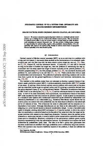
Fig. 1. Vertex-vertex distance distributions in giant components in the real-world networks.

are provided by Newman 1 , Arenas 2 and Leskovec 3 . Please see these web sites for more details. Table 1 shows the basic properties of each network, such as the vertex number |V |, the edge number |E|, the vertex number in the giant component |Vgc | and edge number in the giant component |Egc |, the average shortest path length `, the “harmonic mean” shortest path length `h and the diameter D, etc. 3.3

Vertex-Vertex Distance Distributions

We study the vertex-vertex distance distributions in the giant component Ggc = {Vgc , Egc } of the each network just as the method used by Watts and Strogatz [14]. Table 1 shows the mean shortest path length ` and the “harmonic mean” distance `h of each graph. There still exists significant difference between the values of ` and `h , so we do not regard the ‘harmonic mean” `h as an accurate value to show the ` even if there all the vertices are reachable. Fig. 1 shows the vertex-vertex distance distributions of some real-world networks in Table 1. We also get the mean shortest path ` length and the standard deviation σ of the distance distribution for each network. We find that the vertex-vertex distance distributions in the real-world networks are almost invariably symmetrical. By using the same values of ` and σ, we fit each vertex-vertex distance distribution with a normal distribution with the same values of mean and deviation. 1 2 3

http://www-personal.umich.edu/∼mejn/netdata/ http://deim.urv.cat/∼aarenas/data/welcome.htm http://snap.stanford.edu

6

Q. Ye et al.

To calculate the difference between the normal distribution and the real-world distribution, we also get the the coefficient of determination R2 of these two distributions. To our surprise, we find all the vertex-vertex distance distributions of networks in Table 1 conform well with the fitted normal distributions. The coefficients of determination R2 in the networks which contains more than 1000 vertices are all above 0.97. As shown in Table 1, most of vertex-vertex distances are narrowly distributed near the mean shortest path length `, and most of the standard deviations σ are below 2 except that of the Power-grid network. We also note that for different snapshots of the same network, the vertex-vertex distributions may vary greatly due to the changes of the network sizes, such as the Amazon0302 and Amazon0312 networks.

4 4.1

Sampling Algorithms Sampling Algorithms

Given a graph G = (V, E), an induced graph G[T ] is a subgraph that consists vertex set T and all the edges whose endpoints are contained in T . There are many ways to create a sampled subgraph G0 from the original G(V, E). In the following parts, we will use 4 sampling algorithms called random vertex subgraph sampling, random edge subgraph sampling, snowball subgraph sampling and the random vertex sampling to estimate the mean shortest path length of the original graph. The sampling fraction of the algorithms is defined as the ratio of selected vertices to the total vertex number n in the original graph, and we also just calculate the average vertex-vertex distances in the giant components. – Random vertex subgraph sampling (RVS): Select a vertex set S from the original graph G randomly, and keep the edges among them. The subgraph G0 can be formalized as getting the induced subgraph G0 = G[S] of the vertex set S [10]. – Random edge subgraph sampling (RES): Select edges randomly from the original graph G, and the vertices attached to them are kept. The subgraph G0 containing the links is the sampled subgraph [10]. – Snowball subgraph sampling (Snowball): Select a single vertex from the graph randomly from the original graph and all its neighbors are picked. Then all the vertices connected to the selected ones are selected. This process is continued until the desired number of vertices are selected. To control the number of vertices in the sampled graph, a certain number of vertices are randomly selected from the last layer [10]. – Random vertex sampling (RV): Selecting a vertex set S randomly from the giant component. Perform a BFS computation from each vertex i ∈ S to all vertices in G, and calculate the mean shortest path length. In a sparse graph which contains n vertices and m edges, it takes O(m + n) time by using the Breadth First Search (BFS) algorithm to get all the shortest path lengths from one source vertex i ∈ S to all other vertices. The sampling algorithm takes O((m + n)|S|) = O(n|S|) to the average shortest path in


7

sparse networks. We also note that Leskovec et al. [11] use similar method to get the mean vertex-vertex distance in the MSN network, and Potamias [13] use similar method to calculate the closeness values of vertices. Although these these similar methods have been proposed so far, but none of them has been subjected to strict tests to evaluate their performance. 4.2

Mean and Variance of Random Vertex Sampling

Suppose in a graph G the vertex-vertex distance follows the same distribution with a finite mean ` and a finite variance σ 2 , instead of considering its probability distribution. Let us select k pairwise vertices from the original graph, where k is very large integer. Let D1 , D2 , · · · , Dk to be a sequence of independent and identically distributed pairwise shortest path length random variables. It is easy to prove that the mean pairwise vertices shortest path length also follows the normal distribution with the mean shortest path length `rand =

k X Di i=1

k

→ `,

Pk 2 2 and its variance σrand = i=1 Dki = σk regardless the vertex-vertex distance distributions in the original graphs. By using the random vertex (RV) sampling algorithm, suppose wePselect a vertex i from the original graph and calculating the sum of distances j>i di,j from vertex i to all other vertices. P The mean of the shortest path lengths ì from di,j vertex i to other vertices is ì = j>i . Let us assume all the distances di,j n−1 follow the same distribution with a finite mean ` and a finite variance σ 2 . The mean of all vertex-vertex distances from the source vertex i is ì = l and its σ standard deviation is σi = √n−1 . So we can get that the mean distance `rand P|S| ì of the vertex set S is `rand = i=1 |S| = ` and its standard deviation σrand . We can conclude that the random vertex sampling algorithm is is √ σ |S|(n−1)

a very efficient way to estimate the average shortest path lengths in massive graphs with just selecting a small number of vertices from the original graphs. 4.3

Empirical Study of Sampled Subgraphs

Fig. 2 shows the estimated average shortest path lengths of some networks in Table 1 got by different sampling algorithms, and the horizontal dashed lines are the values for the original mean shortest path length of each network. All the sampling ratios of the four sampling methods are the fraction of the number of chosen vertex number |S| to the total node number |V | in the original graph. Our random vertex (RV) sampling algorithm performs well in all graphs, and the estimated values are almost coincide with the original mean values in all the networks even the sampling ratio is very small. We can also find some interesting characteristics of other 3 sampling algorithms. In all these real-world

Q. Ye et al.

10

20

15

10 RVS RES Snowball RV Original

5

0.1

0.2

0.3

0.4

0.5

0.6

0.7

0.8

6

4

2

0 0

1

6

4

2

0.1

0.2

0.3

0.4

0.5

0.6

0.7

0.8

0.9

0 0

1

0.1

0.2

0.3

0.4

0.5

0.6

0.7

0.8

(a) Power

(b) PGP

(c) CA-GrQc

11

6

9 8 7 6 5

14

RVS RES Snowball RV Original

5.5

10

5

4.5

4

3.5

3

2.5

4

0.2

8

Sampling fraction


0.1

10

Sampling fraction

12

3 0

8

Sampling fraction

13

Mean shortest path length

0.9


12


0 0

14



12

25


30



8

0.3

0.4

0.5

0.6

0.7

0.8

0.9

1

2 0

0.1

0.2

0.3

0.4

0.5

0.6

Sampling fraction

Sampling fraction

(d) Cond-Mat

(e) AS06

0.7

0.8

0.9

1

0.9

1


12 10 8 6 4 2 0

0.2

0.4 0.6 Sampling fraction

0.8

1

(f) HepTh

Fig. 2. Estimated average shortest path lengths according to different sampling ratios of different sampling algorithms. The horizontal dashed lines are the values for the original mean shortest path length of each network.

networks shown in Fig. 2, the average shortest path lengths got by the random edge subgraph (RES) sampling algorithm are usually larger than those got by the random vertex subgraph sampling algorithm. When we get enough vertices in the subgraphs, the estimated mean shortest path length got by the the Snowball sampling algorithm increases with the growing of the sampling fractions. Obviously, for the Snowball sampling, the diameter of the sampled subgraph is expanded gradually from the source vertex as the increasing of the number of vertices. We can also get that the values of estimated average shortest path length got by the random edge subgraph sampling (RES) are usually larger than those got by the random vertex subgraph (RVS) sampling in most cases. To show the stability of the random vertex (RV) sampling algorithm in massive networks, we use the random vertex (RV) sampling algorithm by different sampling fractions to estimate the average shortest path length of the Amazon0302 network and slash8 network, and the results are shown in box plots in Fig. 3. To show the distributions of the estimation mean shortest path lengths in these 2 networks, the sampling the fraction is from 0.01% to 0.1%, and each point in this feature is calculated for 20 times. The horizontal dashed lines are also the values for the original mean shortest path length of each network. We can find that the random vertex (RV) sampling algorithm is very stable, and the median values of the boxes are distributed near the original mean shortest path length. To study the accuracy of the random vertex (RV) sampling algorithm in more networks, we sample 1% vertices from the networks and calculate the


9

4.3



9.1

9

8.9

8.8

8.7

8.6

4.2 4.1 4 3.9

8.5

3.8 1.00E−04

2.00E−04

3.00E−04

4.00E−04

5.00E−04

6.00E−04

7.00E−04

8.00E−04

9.00E−04

0.001

Sampling fraction

(a) Amazon0302

1.00E−04

2.00E−04

3.00E−04

4.00E−04

5.00E−04

6.00E−04

7.00E−04

8.00E−04

9.00E−04

0.001

Sampling fraction

(b) slash08

Fig. 3. Box plots of the changes of mean shortest path length for random vertex (RV) sampling algorithm according to very small sampling ratios of the giant components. The horizontal dashed lines are the values for the original mean shortest path length of each network.

estimated mean shortest path length `0.01 for each network in Table 1. In Table 1 the hyphen character indicates the networks are too small to sample 1% vertices in the giant components. As shown in Table 1, one can see that our random vertex (RV) sampling algorithm matches the experiments very well except when the graphs are very small. 4.4

Model Generated Graphs

We also study the performances of the sampling algorithms for different artificial networks with different pure topological properties. In order to show the phenomena found in real-world networks, many network topology generators have been proposed [1] [2][4][14] [8]. Airoldi and Carley [1] proposed 6 pure topological types: ring lattice type, small world type, Erdös random type, core-periphery type, scale-free type and cellular type. We note that the cellular type models are actually to generate networks with built-in communities, so we call the cellular type model as community type model. To compare the sampling algorithms in these 6 typical topological networks, we choose the ring lattice model [1], Watts & Strogatz small world model [14], Erdös-Rényi random model [1], Albert & Barabasi model [1] [2], core-periphery model [1] and LFR community model [8], respectively. All these algorithms are available in Java in the network analysis framework JSNVA [16] as a part of TeleComVis [15]. To control for possible sources of variations we are not interested, such as the size of the network and density, each generated network contains 1000 vertices. Fig. 4 shows the vertex-vertex distance distributions in the 6 artificial networks. As the ring lattice network is a quite regular network, as shown in Fig. 4(a), almost all the vertex-vertex distances in the network generated by the ring lattice model have the same distribution probabilities, and the probabilities deviate greatly from

10

Q. Ye et al. −3

6

x 10

0.2

5.5

0.18

5

0.16

4.5

0.14

0.4



0.35

4 3.5 3 2.5

Probability

Probability

Probability

0.3

0.12 0.1 0.08

0.25 0.2 0.15

0.06

0.1 2

0.04 Data µ = 125.38,σ = 72.10

1.5 1 0

50

100

150

0.05

0.02

Normal Distribution R2 = −516.9548 200

0 0

250

2

4

6

8

10

(a) Ring Lattice 0.5

0 0

18

2

4

6

8

10

12

Distance

(c) Erd¨ os-Rényi Random 0.8 Data µ = 2.86,σ = 0.57


0.45


0.7


0.4

0.35

0.6

Probability

0.25 0.2 0.15

Probability

0.35

0.3

Probability

16

Data µ = 3.70,σ = 0.87

Data µ = 3.21,σ = 0.87

0.3 0.25 0.2

0.5

0.4

0.3

0.15 0.2

0.1

0.1

0.05 0 0

14

(b) Small World

0.45 0.4

12

Distance

Distance

0.1

0.05

1

2

3

4

5

Distance

(d) Core Periphery

6

0 0

1

2

3

4

5

6

7

Distance

(e) Scale Free

8

9

0 0

0.5

1

1.5

2

2.5

3

3.5

4

4.5

5

Distance

(f) Community

Fig. 4. Mean shortest path length distributions in the of giant components in the sampled networks generated by 6 typical network models.

the normal distribution. However, we can find that the other random networks generated by the other 5 type models, the vertex-vertex distance distributions conform well to the normal distributions. Fig. 5 plots the estimated average shortest path lengths according to different sampling ratios in 6 artificial networks. Each value in Fig. 5 is computed by averaging the observations based on 10 samplings. The result shows that our random vertex (RV) sampling algorithm also perform best in these artificial networks. As shown in Fig. 5, we can also get that in all these typical topological networks the average shortest path lengths got by the random edge subgraph (RES) sampling algorithm are usually larger than those got by the random vertex subgraph (RVS) sampling algorithm. In the ring lattice random network, all of the RVS sampling algorithm, RES sampling algorithm and Snowball sampling algorithm perform bad when the sampling fractions are not large enough. As shown in Fig. 5(a), when the sampling fractions are below 0.6, the estimated shortest path lengths got by the RVS and RES sampling algorithms are still quite small. We also notice the Snowball sampling algorithm perform better than the RVS sampling algorithm and RES sampling algorithm in the other 5 pure topology artificial networks. However, there is a very good agreement between our random vertex (RV) sampling algorithm predictions and the real average shortest path length in each artificial networks. Our random vertex (RV) sampling algorithm performances much better than other sampling algorithms in all the cases both of real-world and artificial networks.


100

50

RNS RES Snowball RN Original

20

15

10

5

16


14 Mean shortest path length

150

25




200

11

12 10 8 6 4 2

0.2

0.4 0.6 Sampling probability

0.8

0 0

1

(a) Ring Lattice RNS RES Snowball RN Original

10


0.8

8

6

4

9

7 6 5 4 3 2

2 0

0.2


0.8

1

(d) Core Periphery

1 0

0.2


0.8

1

(c) Erd¨ os-RényiRandom


8

0 0

1

(b) Small World



12

0.2

10


9 Mean shortest path length

0 0

8 7 6 5 4 3

0.2


0.8

(e) Scale Free

1

2 0

0.2


0.8

1

(f) Community

Fig. 5. Estimated mean shortest path length for each sampling algorithm according to different sampling ratios in the 6 artificial networks. The horizontal dashed lines are the values for the original mean shortest path length of each network.

5

Conclusion

In this paper, we present an empirical study of the vertex-vertex distance distributions in more than 30 real-world networks. Our most striking finding is that in these networks conform well to the normal distributions with different means and variations. As scalability is a key issue for exploring the characteristic path length in massive network exploration, to estimate the average in massive networks, we prove that if the vertex-vertex distances in a network follow the same distribution, we can easily estimate its average shortest path distance accurately by just sampling a small fraction of vertex pairs. We suggest a simple and intuitive sampling algorithm to get the average shortest path length which is very fast and scales well to both of the massive graphs and the different pure topology artificial networks. The results show that we can estimated the average shortest path lengths quickly by just sampling a small number of vertices in massive networks. In real-applications, we can calculate the efficiency of massive networks quickly, such as estimation the efficiency of massive call graphs in real-time.

Acknowledgments We thank M. E. J. Newman, Alex Arenas and Jure Leskovec for providing us the network data sets. This work is supported by the National Science Foundation of China (No. 90924029, 60905025, 61074128). It is also supported the National

12

Q. Ye et al.

Hightech R&D Program of China (No.2009AA04Z136) and the National Key Technology R&D Program of China (No.2006BAH03B05).

References 1. E. M. Airoldi and K. M. Carley. Sampling algorithms for pure network topologies: stability and separability of metric embeddings. SIGKDD Explorations, 7:13–22, 2005. 2. R. Albert and A.-L. Barab´ asi. Statistical mechanics of complex networks. Rev. Mod. Phys., 74(1):47–97, January 2002. 3. R. Albert, H. Jeong, and A.-L. Barab´ asi. Diameter of the world wide web. Nature, 401:130–131, 1999. 4. A.-L. Barab´ asi and R. Albert. Emergence of scaling in random networks. Science, 286:509–512, 15 October 1999. 5. T. H. Cormen, C. E. Leiserson, R. L. Rivest, and C. Stein. Introduction to Algorithms. MIT Press, second edition, 2001. 6. M. Faloutsos, P. Faloutsos, and C. Faloutsos. On power-law relationships of the internet topology. In SIGCOMM ’99: Proceedings of the conference on Applications, technologies, architectures, and protocols for computer communication, pages 251–262, New York, NY, USA, 1999. ACM. 7. J. Kleinberg, A. Slivkins, and T. Wexler. Triangulation and embedding using small sets of beacons. In FOCS, pages 444–453, 2004. 8. A. Lancichinetti, S. Fortunato, and F. Radicchi. Benchmark graphs for testing community detection algorithms. Phys. Rev. E, 78(4):046110, Oct 2008. 9. V. Latora and M. Marchiori. Efficient behavior of small-world networks. Phys. Rev. Lett., 87(19):198701, Oct 2001. 10. S. H. Lee, P.-J. Kim, and H. Jeong. Statistical properties of sampled networks. Phys. Rev. E, 73:016102, 2006. 11. J. Leskovec and E. Horvitz. Planetary-scale views on a large instant-messaging network. In WWW ’08: Proceeding of the 17th international conference on World Wide Web, pages 915–924, Beijing, China, 2008. 12. M. E. J. Newman. The structure and function of complex networks. SIAM REVIEW, 45(2):167–256, 2003. 13. M. Potamias, F. Bonchi, C. Castillo, and A. Gionis. Fast shortest path distance estimation in large networks. In CIKM’ 09, pages 867–876, Hong Kong, China, November 2–6 2009. 14. D. J. Watts and S. H. Strogatz. Collective dynamics of ‘small-world’ networks. Nature, 393:440–442, June 4 1998. 15. Q. Ye, B. Wu, and et al. TeleComVis: Exploring temporal communities in telecom networks. In ECML PKDD, pages 755–758, Bled Slovenia, 2009. 16. Q. Ye, T. Zhu, and et al. Cell phone mini challenge award: Social network accuracy—exploring temporal communication in mobile call graphs. In IEEE VAST08, pages 207–208, Columbus, USA, 2008. 17. U. Zwick. Exact and approximate distances in graphs—a survey. In Proceedings of the 9th Annual European Symposium on Algorithms, pages 33–48, 2001.