Author manuscript, published in "Computational Statistics & Data Analysis / Computational Statistics and Data Analysis 52, 2 (2007) 687-701" DOI : 10.1016/j.csda.2007.03.013
DIVCLUS-T: a monothetic divisive hierarchical clustering method Marie Chavent a,∗, Yves Lechevallier b, Olivier Briant c a IMB,
UMR CNRS 5251, Universit´e Bordeaux1, 351 cours de la lib´eration, 33405 Talence, Cedex, France b INRIA-Rocquencourt,
78153 Le Chesnay, Cedex, France c G-SCOP,
hal-00260963, version 1 - 5 Mar 2008
ENSGI-INPG, 6 avenue F´elix-Viallet, 38031 Grenoble, France
Abstract DIVCLUS-T is a divisive hierarchical clustering algorithm based on a monothetic bipartitional approach allowing the dendrogram of the hierarchy to be read as a decision tree. It is designed for either numerical or categorical data. Like the Ward agglomerative hierarchical clustering algorithm and the k-means partitioning algorithm, it is based on the minimization of the inertia criterion. However, unlike Ward and k-means, it provides a simple and natural interpretation of the clusters. The price paid by construction in terms of inertia by DIVCLUS-T for this additional interpretation is studied by applying the three algorithms on six databases from the UCI Machine Learning repository. Key words: Divisive clustering; monothetic cluster; decision dendrogram; inertia criterion
1
Introduction
The end-point of a classification study is often a partition P of a set of objects Ω into a set of disjoint homogeneous and well separated clusters (C1 , ..., Ck ). When the desired number of clusters k is “high” the aim of clustering is usually to reduce the number of objects. Each cluster is then replaced by its centroid and statistical methods can be applied to the centroids weighted ∗ Tel.: +33 540002116; fax +33 540002626 Email address:
[email protected] (Marie Chavent).
Preprint submitted to Elsevier
12 March 2007
by the number of objects in the corresponding cluster. When the number of clusters k is “small” the aim of clustering is usually to find both homogeneous and interpretable clusters. An additional step of cluster interpretation is then necessary.
hal-00260963, version 1 - 5 Mar 2008
The idea of this article is to propose a monothetic divisive hierarchical clustering method called DIVCLUS-T. Like the Ward agglomerative hierarchical method and the k-means partitioning method, this divisive method is based on the minimization of the inertia criterion, but it provides, by construction, a simple and natural interpretation of the clusters. Divisive hierarchical clustering reverses the process of agglomerative hierarchical clustering, by starting with all objects in one cluster, and successively dividing each cluster into smaller ones. A natural approach for dividing a cluster into two non-empty subsets would be to consider all the possible bipartitions. It is clear that such a complete enumeration procedure provides a global optimum but is computationally prohibitive. A variety of divisive clustering methods which do not consider all bipartitions have been suggested. MacNaughton-Smith et al. (1964) and Kaufman and Rousseeuw (1990) proposed iterative divisive procedures using an average dissimilarity between an object and a group of objects. Other methods using a dissimilarity matrix as input are based on the optimization of criteria such as the split or the diameter of the bipartition (Gu´enoche et al., 1991; Wand et al., 1996). For the inertia criterion, divisive counterparts to Ward’s agglomerative algorithm have been proposed: for example, instead of splitting by total enumeration it is possible to apply the k-means algorithm, with k=2 (Mirkin, 2005). In divisive clustering, some methods are polythetic, whereas some others are monothetic. A cluster is called monothetic if a conjunction of logical properties, each one relating to a single variable, is both necessary and sufficient for membership in the cluster (Sneath and Sokal, 1973). A clustering method which builds, by construction, monothetic clusters is then monothetic. In divisive clustering, monothetic clusters are obtained by using, for each division, a single variable and by separating objects having specific variable values from those who do not. Monothetic divisive clustering methods are usually variants of the association analysis method (Williams and Lambert, 1959) and are designed for binary data. We can cite among others Lance and Williams (1968), Kaufman and Rousseeuw (1990). Unlike the first methods cited above, these monothetic methods are not based on the optimization of a “polythetic” criterion like the inertia or the diameter of the bipartitions. These methods are based on the selection, at each stage, of the binary variable which maximizes a measure of association to the other variables. The objects are then divided using the values (0 and 1) of the binary variable. The divisive clustering method proposed in this paper is monothetic but pro2
hal-00260963, version 1 - 5 Mar 2008
ceeds by optimization of a polythetic criterion. The bipartitional algorithm and the choice of the cluster to be split are based on the minimization of the within-cluster inertia. The complete enumeration of all possible bipartitions is avoided by using the same monothetic approach as Breiman et al. (1984) who proposed, and used, binary questions in a recursive partitional process, CART, in the context of discrimination and regression. In the context of clustering, there are no predictors and no response variable. Hence DIVCLUS-T is a DIVisive CLUStering method whose output is not a classification nor a regression tree, but a CLUStering-Tree. Because the dendrogram can be read as a decision tree, it simultaneously provides partitions into homogeneous clusters and a simple interpretation of those clusters. In Chavent (1998) a simplified version of DIVCLUS-T was presented for the particular case of quantitative data. Chavent et al. (1999) applied it, together with another monothetic divisive clustering method based on correspondence analysis, to a categorical data set on healthy human skin. A first comparison of DIVCLUS-T with Ward and k-means was given in this paper but only for a single categorical dataset and for the 6-cluster partition. More recently, it has been applied to accounting disclosure analysis (Chavent et al., 2005) and a hierarchical divisive monothetic clustering method based on the Poisson process has been proposed in Pircon (2004). In this paper we present the method DIVCLUS-T in detail (section 5). This monothetic Ward-like clustering method can also be applied to categorical data and the calculation of the inertia criterion for categorical data is introduced in section 4. The numerical and categorical examples (sections 2 and 5.3) show that the main advantage of DIVCLUS-T compared to Ward or k-means is the simple and natural interpretation of the dendrogram and the clusters of the hierarchy. Because these monothetic descriptions are also constraints which may deteriorate the quality of the divisions, in section 6 we study the price paid by DIVCLUS-T, in terms of inertia, for this additional interpretation. We compare the inertia of the partitions obtained with DIVCLUS-T, Ward and k-means for the six databases of the UCI Machine Learning repository Hettich et al. (1998).
2
An example
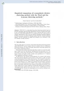
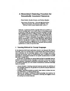
The agglomerative Ward method and the divisive DIVCLUS-T method have been applied to the well-known protein consumption data table (Hand et al., 1994). The dendrogram of the hierarchy obtained with Ward is given in Figure 1. This dendrogram doesn’t give any information about the interpretation of the clusters such as, for instance, that of {Italy, Greece, Spain, Port}. 3
3.12
1.24 0.89 0.74 0.51
Den
Swed
Nor
Fin
Switz
Aust
Nether
Ireland
Belg
W_Ger
UK
Fr
E_Ger
Czech
Pol
USSR
Hung
Port
Spain
Greece Italy
Yugo Rom
Bulg
Alban 3.12
Nuts > 3.5
Yes
No
1.21
Fruits/Veg. >5.35 No
Yes
0.77
Fish>5.7
No
0.56 3.51
Starchy Foods >3.9 Yes No
No
Red Meat > 12.2
Yes
Yes
Den
Swed
Nor
Finl
UK
Ireland
Belg Fr
Switz
Aust
Nether
W_Ger
E_Ger
Czech
Pol
USSR
Port
Spain
Greece
Italy
Yugo
Rom
Bulg Alban
Hung
hal-00260963, version 1 - 5 Mar 2008
Fig. 1. Ward dendrogram for protein data.
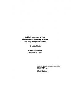
Fig. 2. DIVCLUS-T dendrogram for protein data.
The dendrogram of the hierarchy obtained with DIVCLUS-T is given in Figure 2 and differs from the Ward dendrogram in the inclusion of the monothetic description for each level. For instance, we can read that the countries of the {Italy, Greece, Spain, Port} cluster are characterized by their Nuts and Fruits/Vegetable consumption (Nuts > 3.5) whereas the European countries of the {Fin, Nor, Swed, Den} cluster are characterized by their Fish consumption (Fish > 5.7). The clusters obtained with DIVCLUS-T have natural interpretation but how do the inertias of the clusters obtained by the two methods compare ? In the case of the protein data table, all the countries have the same weight and the inertia criterion is the classical error sum of squares (SSQ) criterion. We 4
see in Table 1 that the proportion of the explained inertia is better for the partitions of DIVCLUS-T from 2 to 4 clusters and better (or equal) for the partitions of Ward from 4 to 10 clusters. The disadvantage, in term of inertia, of being monothetic seems to be counterbalanced by the advantage of being divisive. Note that few cluster partitions are obtained in the first stages of divisive hierarchical clustering whereas they are obtained in the last stages of agglomerative hierarchical clustering. Table 1 Proportion of the inertia (in %) explained by the k-clusters partitions obtained with DIVCLUS-T and Ward on the protein data set
hal-00260963, version 1 - 5 Mar 2008
k
2
3
4
5
6
7
8
9
10
DIVCLUS-T
37.1
50.6
59.2
65.5
71.2
73.5
79.3
81.6
84
Ward
34.7
48.5
58.5
66.7
72.4
75.5
79
81.6
84
3
The data table
We consider a set Ω = {1, ..., i, ..., n} of n objects which are described by p variables X 1 , . . . , X p in a matrix X of n rows and p columns: 1···j ···p 1 .. . X = (xji ) = i .. . n
···
· .. . xji .. . ·
··· .
xji is the value of the jth variable X j for object i. For a numerical variable, xji ∈ R and for a categorical variable, xji ∈ M j , the set of categories of X j . We will denfine by q j the number of categories of X j . Here we do not consider the case of a mixed data table and so the X entries are either all numerical or all categorical. A weight mi is associated to each object i and those weights are organized in a vector m = (m1 · · · mi · · · mn )t . If the data result from random sampling with uniform probabilities, the weights are also uniform : mi = 1/n for all i. But it can be useful, for certain applications, to work with non-uniform weights (reweighted sample, aggregate data). 5
4
The inertia criterion
A general approach for splitting a set Ω = {1, ..., i, ..., n} of n objects into k disjoint clusters involves defining a measure of adequacy of a partition Pk and seeking a partition which optimizes that measure. Several possible measures of adequacy exist (Gordon, 1999; Hansen and Jaumard, 1997) and are used in different clustering methods. Here we have chosen to use the inertia criterion (which is a generalization of the error sum of squares criterion). Note that a k-clusters partition Pk is a list (C1 , . . . , Ck ) of subsets of Ω verifying Cℓ 6= ∅ for all ℓ = 1, . . . , k, C1 ∪ . . . ∪ Ck = Ω and Cℓ ∩ Cℓ′ = ∅ for all ℓ 6= ℓ′ .
hal-00260963, version 1 - 5 Mar 2008
4.1 Definitions
The inertia criterion is defined on a numerical weighted data table (Z, w) associated with a set Ω of n objects as described in section 4.2, where,
1···j ···p 1 .. . Z= i .. . n
···
· .. . zij .. . ·
···
,w=
w1 . . . w i .. .
.
wn
In the calculation of the inertia criterion, an object i ∈ Ω will be weighted by wi and identified with the corresponding row of the matrix Z : zi = (zi1 · · · zip )t ∈ Rp . The inertia of a cluster Cℓ ⊆ Ω is then defined by: I(Cℓ ) =
X
wi d2M (zi , g(Cℓ )),
(1)
i∈Cℓ
where wi is the weight of the object i and g(Cℓ ) is the cluster centroid defined by: X 1 w i zi . g(Cℓ ) = X wi i∈Cℓ i∈Cℓ
6
The distance dM between the two vectors zi and zi′ of Rp is defined by: d2M (zi , zi′ ) = (zi − zi′ )t M(zi − zi′ ),
(2)
where M is a p × p positive definite matrix. If M = I and wi = 1 for all i = 1 · · · n, then the inertia is the classical error sum of squares (SSQ) criterion. The sum of the inertias of all clusters is called the within-cluster inertia: W (Pk ) =
k X
I(Cℓ ) .
(3)
ℓ=1
It is an heterogeneity criterion for the adequacy of a partition Pk = (C1X , ..., Ck ). wi , is Similarly, the inertia of the centroids g(Cℓ ), weighted by µ(Cℓ ) = i∈Cℓ
hal-00260963, version 1 - 5 Mar 2008
called the between-cluster inertia: B(Pk ) =
k X
µ(Cℓ ) d2M (g(Cℓ ), g),
(4)
ℓ=1
with g = g(Ω) the centroid of Ω. This is an isolation criterion for the adequacy of Pk . Finally, because the total inertia of a set of Rp points can be partitioned into within and between-cluster inertia, we have I(Ω) = W (Pk ) + B(Pk ),
(5)
and so minimizing W (the heterogeneity) is equivalent to maximizing B (the isolation).
4.2 The inertia criterion for numerical or categorical data
For a numerical matrix X, the inertia criterion is calculated from the weighted data matrix (Z, w) with Z = X and w = m. Moreover, the matrix M used in the quadratic distance dM defined in (2) is usually the identity matrix I or the diagonal matrix of the inverse of squared standard deviations:
2 1/s1
D1/s2 =
0
7
..
.
0 1/s2p
.
hal-00260963, version 1 - 5 Mar 2008
This latter distance is used when the variables are measured on very different scales. For a categorical matrix X, the inertia criterion is calculated from a weighted data matrix (Z, w) defined as follows. First the matrix X = (xji )n×p is converted into an indicator matrix Q with n rows and q columns where q = Pp j j=1 q is the total number of categories in all variables. In each ith row of the indicator matrix, an element is 1 if the object belongs to the corresponding category s of the corresponding categorical variable; otherwise the element is 0. Thus the sum of all the elements in a row is p, the number of variables. A matrix K = (kis )n×q is obtained by multiplying for all i the ith row of this indicator matrix Q by the weight mi . Because the matrix K can be considered as a kind of contingency table, the matrix of relative frequencies F = (fis )n×q called the correspondence matrix, can be constructed. The relative frequency P P fis is obtained by dividing the frequency kis by k.. = i s kis , the overall total ks frequency: fis = k..i . The second step is to convert the correspondence matrix F ˜ n×q = (˜ ˜ n )t . The ith row profile x ˜ i is then into a row profiles matrix X x1 , . . . , x defined by dividing the ith row of the correspondence table F by its marginal P total fi. = qs=1 fis i.e.: ˜i = ( x
fi1 fq , ..., i ) . fi. fi.
The total marginals of the correspondence matrix F are also used to define the row and the column masses : the vector (f1. , ..., fi. , ..., fn. ) gives the masses of the rows and the vector (f.1 , ..., f.s , ..., f.q ) gives the masses of the columns. Finally the inertia criterion is calculated on the weighted data matrix (Z, w) ˜ and w = (f1. , ..., fi. , ..., fn. )t . Moreover the matrix M used in the with Z = X quadratic distance dM is not the identity matrix I nor the diagonal matrix D1/s2 as for numerical data, but the diagonal matrix of the inverse of columns masses: D1/f = diag(1/f.1, . . . , 1/f.q ).
The resulting distance ˜ i′ ), ˜ i′ )t D1/f (˜ ˜ i′ ) = (˜ xi − x xi − x d2D1/f (˜ xi , x is called the chi-squared distance because, when Kn×q is a real contingency table crossing a set I of n categories with a set J of q categories, the inertia of the n row profiles weighted by (f1. , ..., fi. , ..., fn. ) is identical to chi-square contingency coefficient over k.. . 8
5
DIVCLUS-T
In the divisive hierarchical clustering algorithm, one recursively splits a cluster into two sub-clusters, starting from the set of objects Ω = {1, ..., n}: given the current partition Pk = (C1 , ..., Ck ), one cluster Cℓ is split in order to find a partition Pk+1 which contains k+1 clusters and optimizes the chosen adequacy measure, based on the inertia criterion. More precisely, at each stage, the divisive hierarchical clustering method DIVCLUS-T:
hal-00260963, version 1 - 5 Mar 2008
• splits a cluster Cℓ into a bipartition (Aℓ , A¯ℓ ) of minimum within-cluster inertia. This bipartitional method is defined in section 5.1. • chooses in the partition Pk the cluster Cℓ to be split in such a way that the new partition Pk+1 has minimum within-cluster inertia. This choice is explained in section 5.2, and its link to the construction of the dendrogram is emphasized.
5.1 The problem of how to split a cluster
In order to split optimally a cluster Cℓ one has to choose the bipartition (Aℓ , A¯ℓ ) amongst the 2nℓ −1 −1 possible bipartitions of this cluster of nℓ objects. It is clear that such complete enumeration (EdWards et al., 1965) provides a global optimum but is computationally prohibitive. For some adequacy criteria such as the larger of the two sub-clusters diameters, a polynomial-time algorithm exists for the determination of an optimal division (Gu´enoche et al., 1991). For the inertia criterion, the k-means iterative relocation algorithms, or one of its several variants (Anderberg, 1973), provides at least one locally optimal division. Here, we have chosen to use a monothetic approach to reduce the number of admissible bipartitions. Breiman et al. (1984) proposed and used binary questions in CART a recursive partitioning process in the context of discrimination and regression. Here we use those binary questions in the context of clustering to reduce the set of possible bipartitions.
5.1.1 Inertia of a bipartition Let (Aℓ , A¯ℓ ) be a bipartition of a cluster Cℓ of Ω with Ω described by a numerical weighted data table (Z, w). From (5) we have that minimizing the within-cluster inertia W (Aℓ , A¯ℓ ) is equivalent to maximizing the betweencluster inertia B(Aℓ , A¯ℓ ). Moreover we know that B(Aℓ , A¯ℓ ) can be written 9
as a weighted distance between the centroids g(Aℓ ) and g(A¯ℓ ): µ(Aℓ )µ(A¯ℓ ) 2 B(Aℓ , A¯ℓ ) = d (g(Aℓ ), g(A¯ℓ )). µ(Aℓ ) + µ(A¯ℓ ) M
(6)
This latter criterion is also the between-cluster distance used in the Ward algorithm.
5.1.2 Binary questions The binary questions are formulated in terms of the initial data matrix X. (1) A binary question Q on a numerical variable X j is given by:
hal-00260963, version 1 - 5 Mar 2008
Is X j ≤ c ? This binary question, also denoted by Q = [X j ≤ c], splits a cluster Cℓ into two sub-clusters Aℓ and A¯ℓ such that Aℓ = {i ∈ Cℓ | xji ≤ c} and A¯ℓ = {i ∈ Cℓ | xji > c}. Because c ∈ R, the number of binary questions is infinite but these binary questions induce only a finite number of bipartitions (Aℓ , A¯ℓ ). Let xj(1) , . . . , xj(i) , . . . , xj(nℓ ) be the ordered values of X j on the nℓ objects of Cℓ . Obviously the binary questions [X j ≤ c] induce the same bipartition ({(1), . . . , (i)}, {(i + 1), . . . , (nℓ )}) for all values of c between two consecutive and different observations xj(i) and xj(i+1) . By convention and in order to associate a unique binary question to each bipartition ({(1), . . . , (i)}, {(i+1), . . . , (nℓ )}) the cut values c are defined as the midpoints between two consecutive observations: {c =
xj(i) + xj(i+1) 2
, xj(i) 6= xj(i+1) , i = 1, ..., n − 1}.
Thus there will be a maximum of nℓ − 1 different bipartitions induced by the binary questions on X j . (2) A binary question Q on a categorical variable X j is given by: Is X j ∈ M ? where M ⊂ M j is a subset of categories of X j . This binary question, also denoted by Q = [X j ∈ M], splits a cluster Cℓ into two sub-clusters Aℓ and A¯ℓ such that Aℓ = {i ∈ Cℓ | xji ∈ M} and A¯ℓ = {i ∈ Cℓ | xji ∈ M} where M is the complement of M in M j . Let q j be the number of categories of M j . If M j is ordered there are q j − 1 different bipartitions (M, M ) of M j . j Otherwise, there are 2q −1 − 1 different bipartitions (M, M ) of M j . Because the number of bipartitions (M, M ) of M j is equal to the number of binary j questions [X j ∈ M], there will be a maximum of 2q −1 −1 different bipartitions 10
(Aℓ , A¯ℓ ) of Cℓ induced by those binary questions. This number of bipartitions grows exponentially with q j the number of categories. Up to approximately 13 categories, the totality of bipartitions induced by the variable X j may be considered for optimization. Beyond that point, a pretreatment has to be applied to these categories. One possibility (among others) consists of ordering the categories by a preliminary multiple correspondence analysis of the data table X. If p is the number of variables and q = q 1 +...+q p the total number of categories, we consider the coordinates of the q categories in q − p dimensions. Each dimension defines an order for the q categories and also for the q j categories. There will be q−p different orders of the q j categories and then at most (q j − 1)(q − p) different bipartitions (M, M ) of M j .
hal-00260963, version 1 - 5 Mar 2008
Finally, DIVCLUS-T selects the bipartition of maximum between-cluster inertia (defined in (6)) amongst the bipartitions induced by all of the binary questions on all of the p variables X 1 , ..., X p .
5.1.3 Choice of the binary question We now consider the particular case where two binary questions Q and Q′ ¯′ ℓ ) of the cluster Cℓ which maxiinduce two bipartitions (Aℓ , A¯ℓ ) and (A′ℓ , A mize the between-cluster inertia. In order to choose amongst these two binary questions we introduce a supplementary criterion D. (1) For a numerical binary question Q = [X j ≤c] corresponding to the bipartition (Aℓ , A¯ℓ ) of Cℓ this criterion is defined by: D(Q) =
B j (Aℓ , A¯ℓ ) , I j (Cℓ )
(7)
where the between-cluster inertia B j (Aℓ , A¯ℓ ) and the inertia I j (Cℓ ) are calculated only on the jth column of the matrix Z = X (see section 4.2 for the calculation of the inertia criterion for numerical data). This criterion measures the part of the inertia of the variable X j explained by the partition (Aℓ , A¯ℓ ) of Cℓ . (2) For a categorical binary question Q = [X j ∈M] this criterion is defined by: D(Q) =
X
s∈M j
B s (Aℓ , A¯ℓ ) , I s (Aℓ , A¯ℓ )
(8)
where the between-cluster inertia B s (Aℓ , A¯ℓ ) and the inertia I s (Cℓ ) are calcu˜ (see section 4.2 for lated on the sth column of the row profile matrix Z = X the calculation of the inertia criterion for categorical data). For the sake of ˜ corresponding to simplicity we write s ∈ M j to characterize the column of X 11
categories of X j . Hence D(Q) is the sum, for all categories of X j , of the part of the inertia of the category explained by the bipartition (Aℓ , A¯ℓ ). D(Q) is the relative contribution of the variable X j to the bipartition (Aℓ , A¯ℓ ). In both cases, D(Q) measures a discrimination power for the variable X j with respect to the partition (Aℓ , A¯ℓ ). Finally, when two binary questions Q ¯′ ℓ ) which both maximize and Q′ induce two bipartitions (Aℓ , A¯ℓ ) and (A′ℓ , A the between-cluster inertia, DIVCLUS-T selects the most discriminating one according to this criterion D. 5.2 Selecting the cluster to be split
hal-00260963, version 1 - 5 Mar 2008
A hierarchy H of Ω is a set of clusters satisfying the following conditions (Gordon, 1999): (a) Ω ∈ H; (b) ∅ 6∈ H; (c) the singleton {i} ∈ H for all i ∈ Ω; (d) if A, B ∈ H, then A ∩ B ∈ {∅, A, B}. An indexed hierarchy is a couple (H, h) where h is a mapping from H to R+ satisfying the following conditions: (i) ∀A ∈ H such that h(A) = 0, A is a singleton, (ii) ∀A, B ∈ H, if A ⊂ B, then h(A) ≤ h(B). The common graphical representations of indexed hierarchies are dendrograms. In divisive clustering, the set of clusters obtained after K − 1 divisions is a hierarchy HK whose singletons are the K clusters of the partition PK obtained in the last stage of DIVCLUS-T. In DIVCLUS-T the number 2 ≤ K ≤ n is given as input by the user. Because the resulting hierarchy can be considered as a partial hierarchy halfway between the top and bottom levels, it is referred to as an upper hierarchy (Mirkin, 2005). This upper hierarchy is indexed by h so that in the dendrogram the height of a cluster Cℓ split into two sub-clusters Aℓ and A¯ℓ is (as in Wards method): h(Cℓ ) = B(Aℓ , A¯ℓ ) =
µ(Aℓ ) µ(A¯ℓ ) 2 d (g(Aℓ ), g(A¯ℓ )). µ(Aℓ ) + µ(A¯ℓ )
When the divisions are continued until giving singleton clusters (or clusters of objects with identical descriptions), all of the clusters can be systematically split and the full hierarchy Hn can be indexed by h. When the divisions are not continued down to Hn , the clusters are not systematically split: in order to have the dendrogram of the upper hierarchy HK built by the “top” (the 12
K − 1 largest) levels of the dendrogram of Hn , a cluster represented higher in the dendrogram of Hn has to be split before the others. DIVCLUS-T then chooses to split the cluster Cℓ with the maximum value h(Cℓ ). Consequently because: W (Pk+1) = W (Pk ) − h(Cℓ ) , maximizing h(Cℓ ) ensures that the new partition Pk+1 = Pk ∪ {Aℓ , A¯ℓ } − {Cℓ } has a minimum within-cluster inertia. DIVCLUS-T then uses the same idea as Wards agglomerative clustering method.
hal-00260963, version 1 - 5 Mar 2008
5.3 An example for categorical data
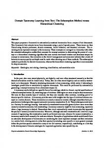
DIVCLUS-T has been applied to a categorical data set where 27 breeds of dogs are described by 7 categorical variables (Saporta, 1990). The number of clusters of the finest partition is fixed to K = 8. The dendrogram of the hierarchy H8 obtained after 7 divisions and the associated 7 binary questions are given in Figure 3. Size
{large}
{small, medium}
Weight
Size {small}
{medium} {very heavy}
{heavy}
Fonction {hunting}
{utility, company}
{fairly intell.} Pekingese
Chihuahua
Teckel
Basset
Poodle
Cocker Spaniel
Dalmatien
Boxer
Bulldog
Brittany Spaniel
Labrador
Saint−Bernard
Bull Mastiff
German Mastiff
Mastiff
Fox−Hound
Levrier
Grand bleu Gascon
Pointer
Setter
French Spaniel
Doberman Pinscher
German Shepherd
Collie
Beauceron
Swiftness {slow} {fast}
Fox Terrier
{very intell.}
Fonction {hunting} {company}
Newfoudland
Intelligence
Fig. 3. DIVCLUS-T dendrogram for dogs data.
At the first stage, the divisive clustering method constructs a bipartition of the 27 dogs. There are 13 different binary questions and 13 bipartitions to evaluate: two variables are binary (inducing two bipartitions), four variables are ordinal with three levels (inducing 4 × 2 bipartitions) and one is nominal 13
with 3 categories (inducing 3 bipartitions). The question “Is size large?” gives the bipartition of smallest within-cluster inertia and is chosen for the first split. For each sub-cluster the “best” bipartition is then obtained in the same way. The between cluster inertia obtained by splitting the 15 “large” dogs is slightly smaller than that obtained by splitting the 12 “small or medium” dogs and so this latter cluster is divided. This process is repeated until we obtain the final 8-cluster partition.
hal-00260963, version 1 - 5 Mar 2008
5.4 Computational complexity
For numerical data the computational complexity of DIVCLUS-T is o(Kpn(log(n)+ p)) with K the number of clusters of the finest partition, p the number of variables, and n the number of objects. Let us briefly compare this complexity with those of Ward and k-means methods. The use of the nearest neighbor method (Mac Quitty, 1966) in agglomerative hierarchical clustering algorithms yields an o(n2 ) implementation of the Ward algorithm, the single-linkage, complete linkage and average linkage algorithms (Benzecri, 1982; Murtagh, 1983; Hansen an Jaumard, 1997). This implementation uses a distance matrix as input. When the input is not a distance matrix but a data matrix (objects×variables), the time spent to compute the distance matrix has to be taken into account. For Ward applied to a quantitative dataset, because the time spent for the calculation of the n(n − 1)/2 Euclidean distances is o(pn2 ), the complexity is o(pn2 ). DIVCLUS-T is then more efficient than Ward for small values of K and p < n. That is explained by the fact that divisive algorithms such as DIVCLUS-T need K − 1 iterations to find the partitions from 2 to K clusters whereas agglomerative algorithms such as Ward need K − n iterations to find the partitions from n to K clusters. The computational complexity of the partitioning k-means algorithm is o(KpnT ), where T is the number of iterations (Duda et al., 2001). DIVCLUS-T is also more efficient than k-means when log(n) + p < T . For categorical data, finding the best bipartition induced by the binary questions can be computationally expensive. In DIVCLUS-T we propose a preliminary treatment which consists of ordering the categories by multiple correspondence analysis of the data table X (see section 5.1.2). By taking this order into account, the number of binary questions on a qualitative variable j X j with q j categories decreases from 2q −1 − 1 to q j − 1 and consequently the set of bipartitions evaluated at each stage is also reduced. The combinatorial problem is then reduced but note that the quality of the best bipartition may be degraded in terms of inertia if the set of possible bipartitions is too small. For qualitative variables with less than approximately 13 categories, complete enumeration is preferred. For ordinal variables there is no combinatorial problem because of the natural order of the categories, but the problem of the 14
quality of the best bipartition in a small set of possible bipartitions remains.
6
Empirical comparison with Ward and k-means
The advantage of DIVCLUS-T in comparison to Ward or k-means clustering methods is the direct and natural interpretation of the clusters. However, what is the price paid by DIVCLUS-T, in terms of inertia, for this additional monothetic description of the clusters ? In order to answer this question, we have applied DIVCLUS-T, Ward and k-means algorithms to three numerical and three categorical datasets of the UCI Machine Learning repository (Hettich et al. (1998)). A short description of the six datasets is given Table 2.
hal-00260963, version 1 - 5 Mar 2008
Table 2 Datasets descriptions Name
Type
# objects
# variables (# categories)
Glass
numerical
214
8
Pima Indians diabete
numerical
768
8
Abalone
numerical
4177
7
Zoo
categorical
101
15(2) + 1(6 )
Solar Flare
categorical
323
2(6) + 1(4) + 1(3) + 6(2)
Contraceptive Method Choice (CMC)
categorical
1473
9(4)
6.1 The proportion of inertia explained
The method DIVCLUS-T uses: - the matrix X to calculate the binary questions and then the set of possible bipartitions at each stage, - a weighted data matrix (Z, w) and a distance dM to calculate the inertia criterion of those bipartitions (see section 4.2): - for the three numerical datasets, Z = X, w = (1, ..., 1)t and M = D1/s2 the diagonal p × p matrix of the inverse of squared standard deviations , ˜ the row profiles matrix, w = - for the three categorical datasets, Z = X t (1/n, ..., 1/n) (because mi = 1 and then fi. = 1/n) and M = D1/f.s the diagonal q × q matrix of the inverse of column masses. The Ward and k-means clustering methods use the same weighted data matrix (Z, w) and distance dM than DIVCLUS-T, but do not use the raw data matrix X within the clustering algorithm. The three clustering methods all use the inertia criterion. Hence the quality of the partitions Pk built by the three methods from the same set of objects 15
Ω, described by the weighted data matrix (Z, w), can be ranked using the proportion E of inertia explained, defined by: E(Pk ) = 100 × (1 −
W (Pk ) ). I(Ω)
(9)
This lies between 0 and 100 (percent) and is equal to 100 for the singleton partition and to 0 for the single cluster (Ω) partition. Because E increases with the number of clusters k of the partition, it can be used only to compare partitions having the same number of clusters. In the following, we assume that a partition Pk is better than a partition Pk′ if E(Pk ) > E(Pk′ ).
hal-00260963, version 1 - 5 Mar 2008
Tables 3 and 4 give partitions from 2 to 15 clusters for the numerical and categorical datasets, respectively. For each dataset the two first columns display the proportion of inertia explained for partitions built with DIVCLUS-T and Ward. The third column displays the proportion of inertia explained for the k-means partitions. Table 3 Numerical datasets: proportion E(Pk ) of inertia explained Glass
Pima
Abalone
k
DIV
Ward
kmeans
DIV
Ward
kmeans
DIV
Ward
kmeans
2
21.5
22.5
22.8
14.8
13.3
16.5
60.2
57.7
60.9
3
33.6
34.1
35.0
23.2
21.6
29.0
72.6
74.8
76.0
4
45.2
44.3
46.6
29.4
29.4
36.2
81.8
80.0
82.6
5
53.4
53.0
54.7
34.6
34.9
41.0
84.2
85.0
86.1
6
58.2
58.4
60.7
38.2
40.0
45.3
86.3
86.8
87.9
7
63.1
63.5
65.7
40.9
44.4
48.9
88.3
88.4
89.6
8
66.3
66.8
68.2
43.2
47.0
51.2
89.8
89.9
90.9
9
69.2
69.2
70.5
45.2
49.1
53.2
91.0
90.9
91.8
10
71.4
71.5
72.4
47.2
50.7
55.1
91.7
91.6
92.4
11
73.2
73.8
74.7
48.8
52.4
56.7
92.0
92.1
92.8
12
74.7
75.9
76.6
50.4
53.9
58.4
92.3
92.4
93.1
13
76.2
77.6
77.2
52.0
55.2
59.7
92.6
92.7
93.4
14
77.4
79.1
78.2
53.4
56.5
61.1
92.8
93.0
93.7
15
78.5
80.4
79.3
54.6
57.7
62.1
93.0
93.2
93.9
First we compare the results for the three numerical datasets (see Table 3). For the Glass dataset the partitions obtained with DIVCLUS-T are either better (for 4 clusters), worse (for 2, 3, and from 12 to 15 clusters) or equivalent (from 5 to 11 clusters). For the Pima dataset the partitions obtained with DIVCLUS-T are better or equivalent up to 4 clusters, and Ward takes the lead from 5 clusters onwards. Because DIVCLUS-T is divisive whereas Ward is agglomerative, it is not really surprising that Ward tends to become better than DIVCLUS-T as the number of clusters increases. For the Abalone dataset which is bigger than the two previous ones (4177 objects), DIVCLUST behaves better than Ward until 3 clusters and the results are very close 16
afterwards. One reason for having better results with DIVCLUS-T on the Abalone dataset is probably the larger number of objects in this database. Indeed the number of bi-partitions considered for optimization at each stage increases with the number of objects. We can then expect better results with larger datasets. For the third column, the k-means algorithm is executed 100 times with different initial seeds and the best solution is retained. Because this algorithm locally optimizes the within-cluster inertia, it is to be expected that the proportion of inertia explained will generally be greater than for the other methods. Finally, for these three continuous datasets, DIVCLUS-T seems to perform better for few cluster partitions and for larger datasets. Table 4 Categorical datasets: proportion E(Pk ) of inertia explained
hal-00260963, version 1 - 5 Mar 2008
Zoo
Solar Flare
CMC
k
DIV
Ward
kmeans
DIV
Ward
kmeans
DIV
Ward
kmeans
2
23.7
22.4
23.7
12.7
12.6
12.7
8.4
7.6
9.1
3
38.2
37.1
38.2
23.8
22.4
23.8
14.0
12.8
15.3
4
50.1
50.3
51.1
32.8
29.3
33.1
18.9
17.3
19.9
5
55.6
55.8
56.5
38.2
35.1
38.6
23.0
21.5
23.9
6
60.9
61.1
61.0
43.0
40.1
43.2
26.3
25.2
27.7
7
65.6
65.5
66.1
47.7
45.0
48.0
28.4
28.5
30.9
8
68.9
68.6
67.1
51.6
49.8
52.1
30.3
30.9
33.7
9
71.8
71.5
69.7
54.3
53.5
55.8
32.1
33.2
36.2
10
74.7
74.4
73.1
57.0
57.1
58.6
33.8
35.5
38.5
11
76.7
76.6
72.9
59.3
60.4
61.4
35.5
37.4
40.3
12
78.4
78.6
77.7
61.3
62.9
64.1
36.9
39.1
42.3
13
80.1
80.1
77.8
63.1
65.2
65.6
38.1
40.6
43.2
14
81.5
81.4
80.1
64.5
67.2
66.6
39.2
42.1
44.4
15
82.7
82.6
81.0
65.8
68.6
68.6
40.3
43.5
46.1
For the three categorical datasets (see Table 4) we obtain the same kind of results. For the Solar Flare and CMC datasets DIVCLUS-T is better than Ward until 10 and 8 clusters respectively. For the Zoo dataset, DIVCLUS-T performs worse than Ward; this may be because all the variables in the Zoo dataset are binary and, as stated before, the quality of the results (in terms of inertia) depends upon the number of categories and variables. These worse results (in terms of inertia) with DIVCLUS-T were to be expected because of the constraint for the clusters to be monothetic. We can however conclude from these examples that in spite of this constraint, DIVCLUS-T performs quite well for few cluster partitions, probably because these arise in the first steps of DIVCLUS-T whereas they come from the last steps of Ward. 17
6.2 Resampling We have used a resampling procedure to go further in the comparison of the three clustering methods. Details on resampling procedures for validation can be found in Mirkin (2005). In our application, the resampling procedure includes the following steps: A. Generation of a number of datasets, copies, by subsampling: a proportion α, 0 < α < 1, is specified and αn objects are randomly selected without replacement as a subsample; data consists of rows corresponding to selected objects. Table 5, gives for each dataset, the size n, the proportion α and the subsample size N = αn. 100 subsamples have been generated for each dataset. Table 5 Subsample descriptions
hal-00260963, version 1 - 5 Mar 2008
Dataset
Dataset size n
Proportion α
Subsample size N
Glass
214
0.70
150
Pima
768
0.65
500
Abalone
4177
0.12
500
Zoo
101
0.79
80
Solar
323
0.62
200
CMC
1473
0.27
400
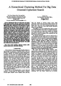
B. Running successively the three clustering algorithms for all 600 copies. C. Evaluating the results for each individual copy. For this, two indices are determined for the partitions from 2 to 15 clusters: - the first index is equal to 1 if the proportion of inertia explained for the partition obtained with DIVCLUS-T is greater than that obtained with Ward. It is equal to 0 otherwise. - the second index is, for each clustering method, the difference between the largest of the three proportions of inertia explained for partitions obtained with the three methods, and the proportion of inertia explained for the partition obtained with the particular method. D. Aggregating results. For each dataset and for partitions from 2 to 15 clusters, the 100 evaluations for each individual copy are averaged. The proportion of subsamples where DIVCLUS-T is better than Ward (in terms of inertia) is calculated by averaging the first index values, see Table 6. The mean deviation of each clustering method from the best solution is given by averaging the second index values, see Figure 4. Table 6 confirms that DIVCLUS-T performs relatively well, despite the monothetic constraint, for few cluster partitions. For the CMC dataset for instance, the two-clusters partition of DIVCLUS-T is better than two-clusters partitions of Ward on 98 subsamples out of 100. Figure 4 shows that the deviation from the best solution is, in the worst 18
Table 6 Percentage of subsamples where DIVCLUS-T performs better than Ward k
2
3
4
5
6
7
8
9
10
11
12
13
14
15
Glass
36
56
59
57
48
41
42
34
25
11
7
5
3
2
Pima
91
36
15
5
1
0
0
0
0
0
0
0
0
0
Abalone
71
21
83
37
22
28
65
50
25
12
7
3
1
1
Zoo
96
88
47
39
43
43
48
63
64
48
47
44
46
43
Solar
91
100
99
100
98
92
71
44
15
2
0
0
0
0
CMC
98
99
100
98
89
61
40
19
9
3
4
1
1
1
GLASS 3 2.5
PIMA 8
DIV WARD KMEANS
7 6
2
5
1.5
4 3
1
2
hal-00260963, version 1 - 5 Mar 2008
0.5
1
0
0 2
4
6
8
10
12
14
16
DIV WARD KMEANS 2
4
6
8
10
ABALONE 3.5
14
16
ZOO 2.5
DIV WARD KMEANS
3
12
DIV WARD KMEANS
2 2.5 1.5
2 1.5
1
1 0.5 0.5 0
0 2
4
6
8
10
12
14
16
2
4
6
8
SOLAR FLARE
10
12
14
16
10
12
14
16
CMC
3.5
5
DIV WARD 3 KMEANS
DIV WARD 4.5 KMEANS 4
2.5
3.5 3
2
2.5 1.5
2 1.5
1
1 0.5
0.5
0
0 2
4
6
8
10
12
14
16
2
4
6
8
Fig. 4. Deviations from the best solution as proportion of explained inertia.
case, equal to 8% of explained inertia (for the PIMA dataset, 7 clusters and DIVCLUS-T). Because the k-means algorithm locally optimizes the inertia criterion, most of the time it gives the best solution. If the k-means partition is the best of the three partitions for the 100 subsamples, its mean deviation is equal to 0. This mean deviation is always close to 0 for the Abalone, Pima and CMC datasets. It is noticeable however that for the other three datasets (Glass, Zoo, Solar Flame) the k-means solution is not always the best and 19
that its deviation from the best solution increases with the number of clusters. Ward even takes the lead from a certain number of clusters onwards. DIVCLUS-T and Ward curves evolve the same way for Glass, Pima, Abalone and Zoo datasets, with Ward above DIVCLUS-T when the number of clusters increases. The deviations of Ward from the best solution are not so different from the deviations of DIVCLUS-T from the best solution for the Abalone and Zoo datasets (except for few cluster partitions). To sum up, it is difficult to conclude from these results that one clustering method is much better than the others in terms of inertia. DIVCLUS-T is not systematically clearly worse than the two other clustering methods. This is, in itself, a reassuring result for this clustering method which allows, by construction, a simple interpretation of the clusters.
hal-00260963, version 1 - 5 Mar 2008
7
Conclusion
This paper proposes a divisive monothetic hierarchical clustering method designed for either numerical or categorical data. For categorical data, the inertia criterion is calculated by converting the data table into a numerical correspondence matrix and a row-profiles matrix. The χ2 distance is then used in place of Euclidean distance. A solution to the computational problem for categorical binary questions is also proposed. The advantage of DIVCLUS-T, compared to classical methods like Ward or k-means, is the direct interpretation of the clusters: the hierarchy can be read as a decision tree. Of course this advantage has to be balanced with a relative rigidity of the clustering process. Some specific simulations should be able to show easily that DIVCLUS-T is unable to find correctly clusters of specific shapes. But what are the shapes of the clusters in real datasets ? We have also seen, on the six datasets from the UCI Machine Learning repository, that the price paid, in terms of inertia, by DIVCLUS-T for the interpretability of the clusters is not systematic, especially for few cluster partitions. Finally, if the user is interested in rather large partitions, for example in order to reduce the number of objects, WARD and k-means are certainly more efficient than DIVCLUS-T. However, if the user is interested in few cluster partitions with good interpretation, DIVCLUS-T seems to be an interesting alternative to classical methods.
References Anderberg, M.R., 1973. Cluster analysis for applications. Academic Press, New York. Benzecri, J.P., 1982. Construction d’une classification ascendante hi´erarchique 20
hal-00260963, version 1 - 5 Mar 2008
par la recherche de chaine des voisins r´eciproques. Les Cahiers de l’Analyse des Donn´ees, VII(2), 209-219. Breiman, L., Friedman, J.H., Olshen, R.A., Stone, C.J., 1984. Classification and regression Trees. C.A:Wadsworth. Chavent, M., 1998. A monothetic clustering method. Pattern Recognition Letters, 19, 989-996. Chavent, M., Guinot, C., Lechevallier Y., Tenenhaus, M., 1999. M´ethodes divisives de classification et segmentation non supervis´ee: recherche d’une typologie de la peau humaine saine. Revue Statistique Appliqu´ee, XLVII(4), 87-99. Chavent, M., Ding, Y., Fu, L., Stolowy, H., Wang, H., 2005. Disclosure and Determinants Studies: An extension Using the Divisive Clustering Method (DIV). European Accounting Review, 15(2), 181-218. Duda R.O., Hart P.E., Strok D.G., 2001. Pattern Classification. WileyInterscience, second edition. EdWards, A.W.F., Cavalli-Sforza, L.L., 1965. A method for cluster analysis. Biometrics, 21, 362-375. Gordon, A.D., 1999. Classification. 2nd Edition, Chapman & Hall/CRC. Gu´enoche, A., Hansen P., Jaumard B., 1991. Efficient algorithms for divisive hierarchical clustering with the diameter criterion. Journal of Classification, 8, 5-30. Hand, D.J., Daly, F., Lunn, A.D., McConway, K.J., Ostrowski, E. (eds.), 1994. A Handbook of Small Data Sets. London: Chapman & Hall. Hansen, P., Jaumard, B., 1997. Cluster analysis and mathematical programming. Mathematical Programming, 4, 215-226. Hettich, S., Blake, C.L., Merz, C.J., 1998. UCI Repository of machine learning databases. http://www.ics.uci.edu/ mlearn/MLRepository.html, Irvine, CA: University of California, Department of Information and Computer Science. Kaufman, L., Rousseeuw, P.J., 1990. Finding groups in data. Wiley, New York. Lance, G.N., Williams, W.T., 1968. Note on a new information statistic classification program. The Computer Journal, 11, 195-197. MacNaughton-Smith, P., Williams, W.T., Mockett, L.G., 1964. Dissimilarity analysis : A new technique of hierarchical subdivision. Nature, 202, 10341035. Mac Quitty, L.L., 1966. Similarity analysis by reciprocal pairs of discrete and continuous Data. Educ. Psych. Meas., 26, 825-831. Mirkin, B., 2005. Clustering for Data Mining. A Data Recovery Approach. Chapman & Hall/CRC. Murtagh, F., 1983. A survey of recent advances in hierarchical clustering algorithms. The Computer Journal, 26, 329-340. Pircon, J.-Y., 2004. La classification et les processus de Poisson pour de nouvelles m´ethodes de partitionnement. Phd Thesis, Facult´es Universitaires Notre-Dame de la Paix, Namur, Belgium. Saporta, G., 1990. Probabilit´es Analyse des donn´ees et Statistique. Editions 21
hal-00260963, version 1 - 5 Mar 2008
TECHNIP. Sneath, P.H., Sokal, R.R., 1973. Numerical Taxonomy. San Francisco, W.H. Freeman. Wang, Y., Yan, H., Sriskandarajah, C., 1996. The weighted sum of split and diameter Clustering. Journal of Classification, 13, 231-248. Williams, W.T., Lambert, J.M., 1959. Multivariate methods in plant ecology. Journal of Ecology, 47, 83-101.
22