Diversity Anonymization in Social Networks - Transactions on Data ...

T RANSACTIONS ON D ATA P RIVACY 8 (2015) 173-215

Analysis and Performance Enhancement to Achieve Recursive (c, l) Diversity Anonymization in Social Networks Saptarshi Chakraborty*, John George Ambooken*, B. K. Tripathy*, Swarnalatha Purushotham* *School of Computing Science and Engineering, VIT University, Vellore - 632014, Tamil Nadu, India Email: [email protected], [email protected], [email protected], [email protected] Abstract. Protecting the identities of the actors along with their sensitive information has become a matter of concern for the organizations which are publishing huge amounts of data every day for the purpose of research. Recent studies have shown that simply removing the sensitive labels associated with the actors do not guarantee their privacy protection. The structural property of the graph associated with the network or the information about the degree of the nodes in it can also be used by an adversary to identify a particular actor. Anonymization algorithms available for social networks are relatively less in number as compared to those for micro-data. The reasons being that the process of anonymizing social networks is much more complex and also as the structural property of the original graph should be taken care and more or less to be retained in the anonymized graph to minimize the loss of information. In recent studies, the original micro-data anonymization concepts of k-anonymity and l-diversity have been extended to the social network environment. The ldiversity model can protect the identity of the users as well as the sensitive labels associated with them. Out of the three different versions of l-diversity available, the recursive (c, l) diversity is much more complex than the mostly handled distinct l-diversity. M.Yuan et al (2013) have developed a recursive (c, l) diversity algorithm using the noise node approach. In this paper, we point out some drawbacks in this algorithm and propose an improved algorithm, which removes these drawbacks and generates the anonymized graph with minimal number of noise nodes. In our approach, we use the noise node addition concept as it retains the structural property of the original graph and also preserves the data utility of the anonymized graph. We have tested our algorithm against several real datasets to justify its efficiency. Also, we have established two theorems in order to establish some characteristics which have been used in support of our claims.

Keywords: Recursive (c, l) diversity, noise node, k-anonymity, l-diversity 173

174

1

Saptarshi Chakraborty, John George Ambooken, B. K. Tripathy, Swarnalatha Purushotham

Introduction

Large number of data is produced everyday by different organizations world over which can be utilized for research purpose in different fields. The rapid growth of Twitter, Facebook, and LinkedIn has catalyzed the data science research. This huge amount of user data can be used by researchers to analyze the user characteristics, global or local trends, community growth etc. The data generated from these websites are not limited to research in social networks; but it can be also used for other purposes like analysis of disease spreading patterns or selection of target audience for any advertisement campaign. But, before publishing this data for such purposes, proper care should be taken so that the identity of the actors along with their sensitive labels is protected. The process called data anonymization takes care of this aspect so that even after publication of data neither the identity nor the sensitive label associated with an actor is disclosed. Several anonymization algorithms have been proposed for relational micro-data. Different anonymization models such as kanonymity [19] and its improved version l-diversity [14] have been proposed. Three different versions of l-diversity have been proposed till now for handling relational data. An improved version of l-diversity model i.e. t-closeness is also proposed [11]. Attackers very often use the non-sensitive attributes of the actors to exploit the sensitive information present in the micro-data. Same approach can be used in exploiting the privacy of the users present in the social network data. If a raw social network graph is published, attackers can very easily link the users and the relationship between them. Structural attack is widely used to exploit the personal information of the users in a social network graph. To prevent identification of the actors from structural attacks, the concept of k-anonymity was introduced [9,12,25,27]. We have used the following motivational example to illustrate the importance of k-anonymity. For example, in Fig. 1 we represent a connection network graph among 10 students of a class. If we publish the graph in Figure 1, then any attacker having the previous knowledge that there is only one student who has maximum number of connections (4 connections), then the attacker can easily identify that the actor represented by node 3 is that particular user. To overcome this problem, the concept of k- degree anonymity was proposed which states that for every node there should be at least k1 other nodes in the graph having the same degree. In Figure 2, we can see that the graph is 2-degree anonymous i.e. for every node; there exist at least 1 other node which is having the same degree. To achieve this, we have increased the degree of node 4 and node 5 by 1. But, the deficiency of this model is that it doesn’t consider the sensitive labels associated with the actors. In Figure 2, the nodes 3 and 5 have

T RANSACTIONS ON D ATA P RIVACY 8 (2015)

Analysis and Performance Enhancement to Achieve Recursive (c, l) Diversity Anonymization in Social Networks

175

the same sensitive label and so an attacker can easily infer that the actors having degree 4 are associated with the sensitive label S1. So, without identifying the particular user, an attacker can extract the personal sensitive information of the actors. To solve this problem, the notion of l-diversity was introduced in [14]. The l-diversity model states that for every equivalence group, there should be at least l distinct sensitive labels. In Figure 3 we illustrate how the graph in Figure 2 can be modified to satisfy 2-degree anonymity and 2 diversity i.e. for every node, there exists at least 1 other node having the same degree and for very equivalence group, at least 2 different sensitive labels are present.

Figure 1: Original graph

Figure 2: 2 degree anonymous graph

Figure 3: 2 degree anonymous 2 diverse graph

Currently three different approaches have been proposed to anonymize a social network graph. These approaches are - clustering, edge-editing approach, and noise node addition. In clustering [3, 7, 9, 23], after the clustering process is over, a sub graph representing a cluster is merged to form a super node. This process is not efficient as the utility of the data in the anonymized graph is diminished. In edge editing technique [8, 12, 20, 23, 25], edges connecting the nodes are added or deleted. But this approach does not ensure the protection of the structural properties of the graph. However, the noise node addition approach [22] is useful for protecting the structural property of the original graph. In this model, noise nodes are added to the existing graph to achieve anonymization for a particular k and l value and then the noise node degrees are adjusted in such a way that they can achieve one of the degrees of the nodes present in the original graph. In order to compare the edge editing approach with the noise node addition approach, we consider the network graph given in Figure 4. Using the edge editing approach we transform it into a 2-degree anonymous 2-diverse graph as shown in Figure 5. Similarly applying the noise node addition approach to the graph in Figure 4, we obtain the 2-degree anonymous 2diverse graph shown in Figure 6. We construct the graph in Figure 5, from Figure 4 by adding an edge connecting node 4 and node 11. This has reduced the distance between node 4 and node 11 by 2. But in Figure 6, we added a noise node in between


176


these nodes and connected the two nodes via the noise node. Therefore, the path length between node 11 and node 4 is changed by only 1. So, we can observe that the noise node approach is more efficient in preserving the structural property of the graph. In our paper also, we have used noise node addition technique to anonymize the raw social network graph. In this paper our main objective is to reduce the number of noise nodes added in [22] for anonymization by proposing new algorithms which ensure the addition of minimal number of noise nodes to achieve recursive (c, l) diversity. To achieve this we first analyze and find deficiencies in the noise node addition approach proposed in [22] and then propose algorithms to overcome these deficiencies. We test our approach with real dataset in order to justify our claim and also to establish its effectiveness. The organization of the rest of the paper is as follows. In section 2, we have discussed briefly on the existing techniques. We provide the problem description in section 3 along with the definition of the key terminologies to be used in this paper. In section 4, we introduce the existing noise node addition approach. Our proposed algorithms are introduced in section 5. In section 6, we have thoroughly analyzed the results obtained and shown the effectiveness of our algorithm. In section 7, we conclude with possible future scope and extensions of our work.


2

Figure 5: Edge editing model Figure 6: Noise node addition model

Previous Works

Merging of two sub-graphs or addition or deletion of edges doesn’t ensure the protection of the sensitive labels and preservation of the utility of the anonymized social network data. In the process of anonymization of a social network unlike relational micro-data, we have to maintain the structural properties to preserve the utility of the anonymized data. Two of the very popular techniques to anonymize a social network graph are clustering and edge editing. In clustering [2, 3, 7, 9, 23], a sub-



177

graph is merged to form a super node and all these super nodes are connected by ‘super edges’. But the data utility is reduced if we use this technique for anonymization. In the edge editing approach [6, 12, 15, 20, 25, 27], edges connecting the nodes are swapped, added or deleted. In cluster based approach, each super node is adjusted to contain at least k number of nodes so that it can satisfy k-anonymity. In [23], a clustering approach is proposed to prevent the disclosure of the sensitive labels. In [9], a heuristic clustering model has been proposed which prevents sensitive information disclosure using sub-graph and vertex refinement concept. In [2, 7] the concept of clustering for bi-partite graphs and interaction graphs have been introduced. In [4], a p-sensitive k-anonymous clustering model has been proposed. As the clustering approach does not retain the structural property of the original graph, mining the anonymized graph may not produce the desired result. Edge editing model is used to protect the sensitive information present in the graph from attackers, who have the background knowledge about the user. In [12], the k-anonymity model for network structure i.e. k-degree anonymity was proposed, which requires that for every node; there exist at least k-1 other nodes having the same degree. In [25], a k-neighborhood model was proposed i.e. for every node, there exist at least k1 isomorphic neighborhoods and this model is further extended in [26], which can also handle l-diversity along with k-anonymity. In [18], the authors proposed a different definition of k-anonymity which is quite strict under some specific conditions and also introduced a flexible definition of (k, l) anonymity. In [27], a different model of k-anonymity was proposed which considers the structural property of the individual nodes. In [20], a random edge swapping model to achieve k-anonymity was proposed. But, edge editing method does not ensure the preservation of the structural properties of the graph. In [1], a different type of attack based on the randomness analysis of the graph has been described. The attacker may add some noise nodes in the raw graph before its publication. To handle this, the noise nodes need to be detected and removed before publishing the graph. In [17], an algorithm was proposed to identify the noise nodes by computing the triangle probability difference between the normal nodes and the noise nodes. In [21], another method was proposed which uses the spectrum analysis method to identify the noise nodes. In [13], an anonymization model was proposed which considers the weights of edges as the sensitive labels and preserves the shortest path length in the anonymized graph. In [15], a brief study is presented on the possibility of an attacker identifying the actors present in a graph, if the attacker knows another graph whose nodes partially overlaps with the other graph. In [24], the authors analyzed the possibility of an attacker using the published information of the actors to access the sensitive or


178


unpublished information of the user while mining the social network data. In [22], a noise node addition approach is proposed which preserves the structural property of the graph along with the sensitive labels associated with it. In this paper, we analyze the deficiencies in the approach proposed in [22] and provide solutions so as to develop an improved recursive (c, l) diversity anonymization procedure such that the number of noise nodes added for anonymization is reduced considerably.

3

Problem Description

In this section, we first define the key terminologies to be used in this paper: Social network graph: A social network graph G ( , , , ) consists of four tuples where V is the set of vertices where each vertex represents a node in the social network. E ⊆ V × V is the set of edges between vertices, denotes the set of sensitive labels associated with the vertices. : V → maps the vertices to their sensitive labels. From Figure 1, {1, 2, …, 10} denotes the set of vertices and S1 and S2 denote the two different sensitive labels associated with it. Equivalence Group: An equivalence group is the set of nodes which have the same degree. For example, in Figure 1, node 1, 2, 6, 7, 9, and 10 form an equivalence group. All these nodes have degree 2. k-degree anonymity l-diversity: An equivalence group is said to satisfy the k-degree anonymity l-diversity if there exists at least k-1 other nodes which are having the same degree and for every equivalence group there exist at least l distinct sensitive labels. A graph satisfies k-degree anonymity l-diversity iff all the equivalence groups satisfy the k- degree anonymity l-diversity condition. The graph in Figure 3 is 2 degree anonymous 2 diverse because for every node present in the graph, there exist at least 1 other node which is having the same degree and for every equivalence group, at least 2 distinct sensitive labels are present. Here, we have used the concept of l-diversity proposed in [2]. So, in the anonymized graph, each node can be identified with a probability less than 1/k and as we have also ensured that every equivalence group is l-diverse, so the sensitive label of a node in an equivalence group can’t be identified with a probability greater than 1/l. To achieve k- degree anonymity as well as l-diversity, we have used the noise node addition concept which retains the structural property of the original graph. We have tried to add the noise nodes in such intelligent manner so that the average path



179

length (APL) of the anonymized graph remains almost unchanged. The equation of APL can be defined as: =

2 ( − 1)

∀

,

∈

( ,

);

Where, N denotes the total number of nodes of a graph, , denotes the distance between the node and . Sensitive degree Sequence: We have borrowed the concept of sensitive degree sequence from [12]. Let’s say every node in a graph can be represented by three tuples: (id, d, S); where id denotes the node id, d denotes the degree of the node and S denotes the sensitive label associated with the node. Now, Sensitive degree sequence is defined as the non-decreasing degree sequence of the nodes in a graph. For Fig. 1, the sensitive degree sequence is: (3,4, #1), (4,3, #2), (5,3, #2), (8,3, #1), (1,2, #1), (2,2, #2), (6,2, #2), (7,2, #2), (9,2, #1), (10,2, #2)

k-anonymous l diverse Sequence: A sensitive degree sequence P is a k-anonymous ldiverse sequence if every equivalence group * satisfies the following constraint: 1) All the elements in * are of the same degree i.e. P[ix].d = P [ix +1].d = … = P [ix + n].d 2) * contains at least k number of elements. 3) * should satisfy l-diversity constraint i.e. it should contain at least l distinct labels. The sensitive degree sequence (3, 5, Q), (4, 5, P), (1, 4, Q), (5, 4, P), (2, 3, P), (7, 3, Q) is a 2 anonymous 2 diverse sequence. In this sequence, every equivalence group contains at least 1 node which has the same degree and also each equivalence group contains at least 2 different sensitive labels. Using the above concepts and terminologies, we can generate the recursive (c, l) diverse anonymized graph which can retain the structural property of the original graph after anonymization as proposed in [22]. The anonymized graph generation process can be divided into two sub steps: 1) Recursive (c, l) diverse sequence generation: In this step, we first generate the sensitive degree sequence of the given graph and then compute the recursive (c, l) diverse sequence for a pre-given c and l value. In the next step, we construct a graph which satisfies the target degrees obtained from the recursive (c, l) diverse sequence by adding noise nodes. 2) Graph construction algorithm: In this step, we have used the algorithms proposed in [22] to generate the anonymized graph using noise node addition approach. In this paper, our sole objective is to reduce the number of noise nodes added to achieve recursive (c, l) diversity. So, firstly we have studied the graph construction algorithm for recursive (c, l) diversity proposed in [22], and identified the deficien-


180


cies in their approach. To overcome those limitations and also to reduce the number of noise nodes, we have proposed new algorithms to achieve recursive (c, l) diverse anonymization. In the following section, we have provided a brief study on the algorithms proposed in [22].

4

Existing noise node addition approach for recursive (c, l) diversity anonymization

In this section of our work, we have discussed about recursive (c, l) diversity model and also the graph construction algorithms by adding noise nodes to achieve recursive (c, l) diversity anonymization.

4.1

Recursive (c, l) diversity Model

Recursive (c, l) diversity model is a complex version of l-diversity model proposed in [14]. It states - For any equivalent group G, if there are m different sensitive labels present, then the group satisfies recursive (c, l) diversity for a pre-given c and l value, if the following condition is satisfied: +, < .(+/ + +/1, + ⋯ + +3 ). In [22], the authors proposed some extra conditions termed as safety grouping condition and added two more conditions in the existing recursive (c, l) diversity criteria. The constraints for satisfying safety grouping condition are: 1) C ≥ k; 2) +, < .(+/ + +/1, + ⋯ + +3 ); 45 1, < . 3) 4 (36/1,) 5

Any group which satisfies the safety grouping condition automatically satisfies the recursive (c, l) diversity condition [22]. The following algorithm was proposed in [22] to generate recursive (c, l) diversity degree sequence. Algorithm Input: raw social network graph data Output: Recursive (c, l) diverse sequence = 7ℎ9 :9 :;7;99 :9?@9 .9 A+ 7ℎ9 A>;=; BC =>BDℎ E, #97 F = { }; IJKLM | | > 0 PQ E>A@D R = { S0T}; ; 7 = S0T. ;



181

F9VAA@D; = RA ;7;A )PQ YQZ ; = 0; ; < | |; ; + +PQ KY S;T. ≡ \JM] R = R ∪ { S;T}; F9VAB .9 CBc9C :97 A+ R \JM] R = R ∪ { S;T}; F9VA=97 9=>99: A+ 9=>99: A+ 9C9V9 7: ; R B: .A>>9:D; ; = A 9: V9B 9=>99; RADX R ; 7A ;+ R :B7;:+;9: #E .A ;7;A ; ::;= 7ℎ9 9C9V9 7: ; F 7A 9d;:7; = =>A@D:;

4.2

Graph construction algorithms

After obtaining the recursive (c, l) diverse sequence, the graph construction algorithm constructs a graph in which all the nodes achieve their respective target degree obtained from the recursive (c, l) diversity sequence generation algorithm. The graph construction process can be divided into four steps:

4.2.1

Step 1: Neighborhood edge editing technique

In this step, the algorithm adds or deletes edges in the neighborhood of a node so that the APL changes by only 1. The three different scenarios which can occur in this step are: Case 1: Node v needs to decrease its degree and u needs to increase its degree and u and v are direct neighbors. So, we randomly chose one direct neighbor w of v which is not connected to u. Remove the edge connecting v and w and add an edge connecting u and w. Algorithm

YQZ 9B.ℎ A 9 @ 99 7A ; .>9B:9 9=>99 PQ = @e : 9=>99; e = @e : 7B>=97 9=>99; YQZ ; = 0; ; < e − ; ; + + PQ fK]P 99 PQ KY @, < B>9 2 ℎAD 9;=ℎcA>: \JM] KY @, < A A7 ℎB9B:9 9=>99 PQ YQZ 9B.ℎ A 9 < 99 7A 9.>9B:9 9=>99 PQ KY @, < ℎB \JM] C; h @, < ;

Figure 7: Case 1

4.2.2

Figure 8: Case 2

Figure 9: Case 3

Step 2: Adding noise node to decrease degree

In this step, the algorithm adds noise nodes to the nodes which need to decrease its degree to achieve the target degree. The process of adding noise node is described below: • Create a new node and connect it with the node which needs to decrease its degree.



183

•

Now, if the node needs to decrease its degree by n, then delete (n+1) edges connecting the node with the other neighboring nodes and connect all those neighboring nodes with the noise node. Algorithm

YQZ 9X A 9 @ 7ℎB7 99 7A 9.>9B:9 7ℎ9 9=>99 PQ = @e : 9=>99; 7B>=97 = 7ℎ9 7B>=97 9=>99 A+ @; IJKLM 7>@9 PQ :9C9.7 B :9 :;7;;=; BC A 9 ℎAD 9;=ℎcA> .>9B79 B 9g A 9 g;7ℎ :9 :;7;99_m _E>A@D( + 2 − (7ℎ9 7B>=97 9=>99)); .A 9.7 A 9 @ g;7ℎ ; = + 1; IJKLM 7>@9 PQ >B AV :9C9.7 B C; h(@, =97 \JM] _ZM`a; KY == 7B>=97 \JM] _ZM`a;

4.2.3

Step 3: Adding noise node to increase degree

In this step, the nodes which need to increase their degree to achieve the target degree are adjusted by the addition of noise nodes. The algorithm involves the following steps: • If a node u needs to increase its degree, then a single noise node is created and it is connected to u. If any node which is within two hop of u also requires increasing its degree, then it is connected with the same noise node. The above process is continued until u achieves its target degree. • If the degree of the noise node is not present in the sensitive degree sequence, then the last connection is deleted until the degree of the noise node matches with a degree in the sensitive degree sequence. Algorithm

YQZ 9X A 9 @ ; E gℎ;.ℎ 99 : 7A ; .>9B:9 ; 9=>99 PQ YQZ ; = 0; ; < ; .>9B:9_ @V; ; + + PQ .>9B79 B 9g A 9 ; .A 9.7 A 9 @ g;7ℎ ; YQZ 9X A 9 < 7ℎB7 ;: A 9 A> 7gA ℎAD 9;=ℎcA> A+ A 9 @ PQ


184

Saptarshi Chakraborty, John George Ambooken, B. K. Tripathy, Swarnalatha Purushotham KY < 99 : 7A ; .>9B:9 ;7: 9=>99 \JM] .A 9.7 A 9 < g;7ℎ ; IJKLM e : 9=>99 ;: A7 ; e ∧ e : 9=>99 O min =>A@D 9=>99 PQ >9VA9B79 7A ; ; ; 1;

4.2.4

Noise node degree setting

In this step, if the noise node degree is not present in the sensitive degree sequence, then we adjust the noise node degree as follows: • Find all the nodes which are within three hopes of the noise node which need to modify its degree • Set a degree which is present in the degree sequence and even times greater than the noise node degree as the target degree of the noise node. • Delete the edge connecting the nodes which are within three hops of the noise node and connect those two nodes with the noise node. Continue the process until the noise node achieves the target degree. Algorithm

:9C9.7 DB;>: A+ A;:9 A 9: 78B7 9B.8 DB;>: A+ A 9: B>9 g;78; 3 8AD: 7A 9B.8 A789>; c@;C B C; h +A> 9B.8 DB;>; YQZ 9X A 9 8B: 999 PQ :9C9.7 B 999 7B>=97 ij . - 7B>=97 ij ; ij ; YQZ 9X A 9 8B: A 9=>99 PQ :9C9.7 B A 9=>99 7B>=97 ij . - 7B>=97 ij ; ij ; YQZ 9B.8 A;:9 A 9 PQ IJKLM . s 7B>=97 ij PQ 0 t >9 7 =>BD8 g89>9 @ B 2 B>9 A7 .A 9.79 7A ; >9VA2. Now, if case1 is applied first on node1and node2, then we have to take extra care so that the edge connecting the node2 and node4 is not deleted and same condition applies if case1 is applied first for node2 and node4. But, if we apply case2 on node1 and node4 first, then we don’t have to check the edge deleting constraint every time. So, applying case2 first saves a lot of computational cost. So, for any scenario which satisfies the above criteria, case2 should be given priority over case1.

5.1.2

Comparative study between case 1 and case 3

Here, we discuss the effect of ordering in between case1 and case3 through different scenarios and show why there should be an ordering between case1 and case3.

5.1.2.1

Scenario 1

The graph in Figure 28 depicts a scenario where case1and case3 can be applied simultaneously. We have considered the structure of this graph to analyze the priority order of case1 and case3. Operation 1: Figure 30 shows the result of applying case1 first. If case1 is applied first on the graph in Figure 30, then it can be done between either node1-node2 or node2-node4. If case1 is applied on node1-node2, node1’s degree will decrease and node2’s degree will be increased. So, node2 will be connected with a neighboring node (u) of node 1 and the edge connecting node u and node1will be deleted. Now only, node 2 needs to increase its degree by 1 and node 4 needs to decrease its de-



191

gree. So, there is no scope of applying case3. Only case1 can be applied. Figure 31 shows the result after applying case1. As a result, no node is left which needs to decrease or increase its degree.


Figure 29: Applying case3 on Figure 28

Figure 30: Applying case1on Figure 28

Operation 2: Figure 29 shows the resulting graph if case3 is applied first. As per the condition of case 3, the degrees of node1 and node 4 will be decreased by one and the edge connecting them is to be deleted. Now, as shown in Figure 29 there isn’t any node left which needs to decrease degree, so there is no scope of applying case 1. The only way to increase the degree of node2 is by adding noise node which will be handled in the next algorithm i.e. addition of noise node to increase the degree. So, from the comparative analysis of both the operations, we can easily conclude that applying case1 first on the above scenario produces better result as compared to case3. So, case1 has more priority in this scenario.


Figure 32: Graph for scenario 2

Figure 33: Graph for scenario 3


192

5.1.2.2


Scenario 2

The graph in Figure 32 describes the scenario where node1, node2 and node4 need to change their degree by 1. Now, if case 1 is applied first, then node 2 will achieve its target degree along with either node 1 or node 4. The remaining node can only achieve their target degrees by the addition of noise nodes. Same result can be obtained if we apply casse3 first. Then, node 1 and node 4 will achieve their target degrees but node2 will require addition of noise nodes to achieve its target degree. So, in the above scenario where all nodes are required to change their degree by 1, case1 and case3 both produce the same output and the computation cost is also same.

5.1.2.3

Scenario 3

Figure 33 describes the scenario where all the nodes need to modify their respective degrees by 2 to achieve the target degrees. Operation 1: If case1 is applied on the graph in Figure 33, then any one of the two combinations node1-node2 or node2-node4 can be chosen. If case 1 is applied on node1 and node2, then the edge connecting node1 with one of its neighbor (u) will be deleted and node u will be connected with node 2 (See Figure 34). If case 1 is applied again on the resulting graph shown in Figure 34, then again we can choose anyone of the combinations node 1-node 2 or node 2-node 4. If we proceed with node 1-node 2, then node 1 and node 2 will reach its target degree but node 4 will require addition of noise nodes to reach target degree (See Figure 35). But if we have chosen node2-node4, then node2 will achieve its target degree but node1 and node4 will still require decreasing their degrees by 1 to achieve the target degrees which can be handled by case3. The main problems of operation1 are: 1) In every application of case1 we have to ensure that the edge connecting node 1 and node 4 does not get deleted, 2) After applying case1 for the first time we have to choose the combination of node 2-node 4 so that the optimal result can be obtained, otherwise noise nodes will be required to achieve the target degree.




193

Figure 35: Applying case 1 on Figure 36: Applying case3on Figure 34 Figure 33

Operation 2: If case3 is applied first on the graph in Figure 33, then the edge connecting node1 and node 4 will be deleted and now only case1 can be applied on the rest of the nodes (See Figure 36). If case1 is applied on node 1 and node 2, node 1 will reach its target degree (See Figure 37) and if case1 is applied once more on node 2 and node 4, then both of them will also reach their respective target degrees (See Figure 38). No extra checking constraint is required in operation 2. From the above analysis of the two operations, we can conclude that operation 2 is a better approach than operation1 because it guarantees producing the optimal output while there is no certainty of getting the optimal output in operation1 and also if we consider computing cost, operation 2 is much more efficient.

5.1.2.4

Scenario 4

The graph in Figure 39 describes a scenario where node 1 and node 4 need to reduce their degrees by 2 and 1 respectively to achieve their target degrees and node 2 needs to increase its degree by 1 to reach its target degree. Operation 1: If case1 is applied first on the graph in Figure 39, then it can be applied on either node1-node2 or node2-node4. If case 1 is applied on node1 and node2, then node1 will decrease its degree by 1 and node2 will increase its degree by 1 and node2 will achieve its target degree. But we have to ensure that while decreasing node 1’s degree, the edge connecting node1 and node4 is not deleted. Otherwise, case3 can’t be applied between node1 and node4. Otherwise, if case 1 is applied on node2 and node4 first, then both of them would have reached their respective target degrees but there wouldn’t be any possibility left for node1 to achieve its target degree by neighborhood edge editing approach. Addition of noise nodes will be the only option.


194



Figure 38: Applying case1on Figure 39: Graph for scenario 4 Figure 37

Figure 40: Applying case3 on Figure 41: Applying case1on Figure 39 Figure 40

Figure. 42: Graph for Scenario 5

Operation 2: Now if case3 is applied first, then node 1 and node 4’s degree will be decreased by 1 and node 4 will be achieving its target degree (See Figure 40). Only node 1 and node 2 will be left which can be handled by case1. After applying case1, both of them will also be reaching their respective target degrees (See Figure 41). So, comparing both the operations, we conclude that operation 2 is more efficient in producing the optimal output and requires less computation cost. Operation 1 does not ensure the optimal output (the graph which will require no noise node addition for anonymization).

5.1.2.5

Scenario 5

The graph in the Figure 42 shows that, node1 and node4 need to decrease their degrees by m and p respectively and node2 needs to increase its degree by n to achieve the target degree, where {m, n, p} >2. Now, if we apply case 1 first on node1and node2, then we have to take extra care so that the edge connecting the node1 and



195

node4 is not deleted and same checking constraint is applied if we are applying case 1for node2 and node4. But, if we apply case3 on node1 and node4 first, then we don’t have to check the edge deleting constraint every time. So, applying case3 first saves a lot of computational cost and hence under any scenario which satisfies the above criteria, case3 should be preferred to case1.

5.1.3

Comparative study between case 2 and case 3

The graph in Figure 43 depicts a scenario where case 2 and case 3 exists simultaneously. Now, if we apply case 2 first, then the two nodes which need to increase their degrees will achieve their target degrees and then if we apply case3 for node1 and node 4, both of them will achieve their respective target degrees by deleting the edge connecting them. Now, if we have applied case 3 first and then case 2, the final output would have been the same. Here, we have taken the example where the nodes need to change the degree by 1. The result shows that the final output is independent of the order of the cases. This is true not only for degree change by 1 but for any n, where n = the amount of degree to be modified for a particular node.

Figure 43: Graph explaining case2 and case3

5.2

Analysis of the result of the comparative study

From the above analysis we can infer the following key points: • The number of noise nodes added for anonymizing the raw social network graph varies with the ordering of applying case 1–case 2 and case1-case3 but it does not depend on the order of applying case 2-case 3. • Among the three cases, following six different combinations can be generated: 123, 132, 231, 213, 312, and 321. But from the analysis we have found out that case 2 and case 3 have no priority order between them. So, applying


196


case 2 before case 3 or case 3 before case 2 doesn’t affect the number of noise nodes added i.e. the output produced by the combinations 123 and 231 are identical with the output produced by 132 and 321 respectively. As a result, we can reduce the problem size to deal with the following four combinations of case orderings- 123, 213, 321, and 312. Our analysis shows that number of noise nodes added is influenced by the ordering of the cases but it does not predict which will be the optimal ordering to obtain minimal number of noise nodes because the number of noise nodes added is governed by the algorithms described in sections 4.2.2 and 4.2.3. So, in the next section, we analyze these two algorithms to predict the optimal ordering which requires addition of minimum number of noise nodes for anonymization.

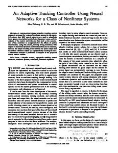
5.3 Analysis of noise node addition algorithms and their effects on noise node addition 1) Now, from Figure 10 describing algorithm (noise node addition to reduce degree), we can observe that for a particular node to reduce its degree, only one fake node is required. The algorithm works in such an intelligent way that the addition of fake nodes is independent of the number of degree changes required for a particular node. So, if there are N nodes which need to decrease their degrees, then N fake nodes will be added. 2) Next, we have analyzed the algorithm (noise node addition to increase degree) to identify the influence of the number of nodes which need to increase their degrees and total amount of degree changes by those nodes on the number of noise nodes added. For this purpose, we have proved two theorems which can be used to generate the optimal case ordering (See the APPENDIX for their proofs). Theorem 1: The minimum number of noise nodes required to be added in the algorithm (Noise node addition to increase degree) is equal to the ceiling of the average degree change required by the nodes which need to increase their degrees and the minimum number of noise nodes occur only when all those nodes are interconnected (one hop or two hop neighbor of each other). Theorem 2: The maximum number of noise nodes required to be added in the algorithm (Noise node addition to increase degree) is equal to the summation of the degree change required by all the nodes which need to increase their degrees to achieve their target degrees.



197

Figure 44: Nodes which need to increase degree

Figure 45: Applying algorithm in step3 on Fig. 44

Figure 46: Applying algorithm in step 3 on Figure 45

Fig. 47: Applying algorithm in step 3 on Figure 46

So, from the above two theorems, we can conclude that if total m number of degree changes is required to achieve the target degree for N number of nodes, then maximum m number of fake nodes need to be added i.e. in the worst case, the no of fake nodes required to be added will be equal to the sum of the degree changes required for all those nodes which need to increase their degrees and the minimum number of fake nodes required will be the ceiling of the average degree change required to achieve the target degree by the nodes which needs to increase their degrees by the addition of fake nodes. Let’s say, each N node needs to increase its degree by m to achieve its target degree. So, the minimum number of fake nodes to be added to achieve the target degree is ⌈ V ⌉. e.g. - let’s assume that four nodes need to increase their degree by 12 to achieve their target degree (See Figure 44). Using the graph in Figure 44, we will be showing an example that the minimum number of noise node addition will occur when each of them needs to modify their degrees by the same amount and the minimum number of noise node is equal to the ceiling of


198


the average degree change. The graphs in Figure 45, 46 and 47 describe the noise node addition approach. All the nodes from node1 to node4 need to increase their degrees by 3 and all of them are one or two hop neighbors of each other. The final output i.e. Figure 47 shows that 3 noise nodes have been added to achieve the respective target degree of all the nodes. If we follow the same procedure where node 1, node 2, node 3 and node 4 needs to increase their degree by 6, 3, 2, and 1 respectively, then at least 6 noise nodes will be required. We can further extend this concept to state that the maximum number of noise nodes to be added is equal to the summation of degree changes required by all the nodes which need to increase their degrees.

5.4

Algorithm 1: Optimal case ordering

In this section we propose an algorithm to compute the optimal ordering of the cases using the results of the Theorems in section 5.3. Let’s say, V denotes the best case of the algorithm (noise node addition to increase degree) i.e. minimum number of addition of noise nodes i.e. ceiling of the average degree change required for all the nodes which need to increase their degrees to achieve the target degrees (See Theorem 1), denotes the number of nodes which need to decrease their degrees to achieve their target degrees, and D denotes the number of noise nodes to be added in the worst case of the ‘noise node addition to increase degree’ algorithm i.e. total number of degree changes required by the nodes which needs to increase their degrees (See Theorem 2). After applying the neighborhood edge editing algorithm for the four different combinations, we can use the following algorithm to find the best case ordering and use that case ordering in the neighborhood edge editing algorithm to generate the anonymized graph with addition of minimum number of noise nodes. The algorithm works in the following way: • Step 1: If for all the case orderings, if the minimum number of noise nodes to be added for the nodes which need to increase their degrees is not less than the number of noise nodes to be added for the nodes which need to decrease their degrees to achieve the target degrees, then select the case ordering which produces minimum number of nodes which needs to increase their degrees. • Step 2: Otherwise, if for all the case orderings, if the number of noise nodes to be added for the nodes which need to decrease their degrees to achieve the target degrees is greater than the minimum number of noise nodes to be added for the nodes which needs to increase their degrees, then select the case ordering which produces the minimum summation of n and p.



199

•

Step 3: Otherwise, calculate the best case orderings which satisfy the condition V ≥ and the condition V - respectively. Select both the best cases as a set of optimal case ordering and compute the graph construction algorithm for both the cases. One of them will produce the anonymized graph with minimum number of noise nodes being added. Algorithm Input: The number of nodes which need to increase or decrease their degree Output: optimal ordering of the cases 1. KY V ≥ +A> BCC 789 .B:9: \JM] 2. :9C9.7 789 .B:9 A> 9>; = g8;.8 D>A @.9: V; ;V@V @Vc9> A+ A 9: g8;.8 99 : 7A ; .>9B:9 789;> 9=>99 3. MLbM KY V - +A> BCC 789 .B:9: \JM] 4. .AVD@79 789 :@VVB7;A A+ B D 5. :9C9.7 789 .B:9 A> 9>; = g8;.8 D>A @.9: V; ;V@V :@VVB7;A 9 V ≥ B V 9. 9 A+ YQZ 10. :9C9.7 789 .B:9 A> 9>; = g8;.8 D>A @.9: V; ;V@V @Vc9> A+ A 9: g8;.8 99 7A ; .>9B:9 9=>99 B :B7;:+;9: 789 .A 7;A V ≥ 11. :9C9.7 789 .B:9 A> 9>; = g8;.8 D>A @.9: V; ;V@V :@VVB7;A AV :79D 10 B :79D 11 B: B :97 A+ AD7;VBC .B:9 A> 9>; = 13. 9 KY

5.5

Algorithm 2: Noise node degree modification

In [22], the main deficiency of the recursive (c, l) diversity graph generation algorithm is that it ignores the possibility of noise node decreasing its degree to reach the target degree. In the algorithm (noise node degree setting); the authors have only proposed the algorithm to modify the noise node degrees by increasing their respective degrees by an even number. If the noise node can’t achieve any of the degree in the degree sequence by increasing its degree in the multiple of 2, then its target degree should be changed by increasing one of the target degrees by 1 and the entire anonymized graph construction algorithm should be computed from the start again. This is the main drawback of the graph construction algorithm proposed in [22] as it requires more computational cost. So, every time we have to consider the whole in-


200


put size and execute all the algorithms. But in our proposed algorithm, we only consider the particular noise nodes which can’t achieve their target degrees after applying noise node degree setting algorithm and apply the graph construction algorithms explicitly for those noise nodes only; not for the entire input size. Algorithm Input: Raw graph data Output: Anonymized graph consisting of noise nodes 1. #97 { } 2. YQZ ; 0; ; < | A;:9 A 9:|; ; + + PQ 3. KY 9=>99[ A;:9_ A 9[;]] ;: A7 D>9:9 7 ; 789 :9 :;7;99 :9?@9 .9 \JM] ∪ A;:9_ A 9[;] 4. 5. 9 KY 6. 9 A+ YQZ 7. IJKLM | |! y PQ 8. 9;=8cA>8AA 9 =9 9 ;7; = +A> 789 9C9V9 7: ; ; 9. A;:9 A 9 B ;7;A 7A 9.>9B:9 9=>99 +A> 789 9C9V9 7: ; ; 10. A;:9 A 9 B ;7;A 7A ; .>9B:9 9=>99 +A> 789 9C9V9 7: ; ; 11. A;:9 A 9 9=>99 :977; = +A> 789 9C9V9 7: ; ; { }; 12. #97 13. YQZ ; 0; ; < | A;:9 A 9:|; ; + + PQ 14. KY 9=>99[ A;:9_ A 9[;]] ;: A7 D>9:9 7 ; 789 :9 :;7;99 :9?@9 .9 \JM] 15. ∪ A;:9_ A 9[;] 16. 9 KY 17. 9 A+ YQZ 18. 9 A+ IJKLM

6

Experimental Results

In this section, we thoroughly analyze the experimental results and show the effectiveness of our algorithms. The results also justify our claim of using an optimal ordering of the cases in the neighborhood edge editing algorithm to obtain the anonymized graph by adding minimal number of noise nodes.

6.1

Dataset

We have used the following three social network datasets:



201

1. The Prefuse project - The dataset consists of 129 nodes. We have considered the first letter of the name of the actors as the sensitive label associated with that actor [10]. 2. Co-authorship Network Data - We have used a co-authorship network data of scientists who were working on network theory and experiments. This dataset was compiled by M. Newman [16]. This particular version, which we have used for our experiment purpose consists of 1589 nodes and 2742 edges. We have considered the first letter of the name of the scientists as the distinct sensitive labels for our experiment purpose e.g. - the sensitive label assigned for the name, KUPERMAN is K. So, 26 different sensitive labels are available. 3. The Cora Dataset (http://www.cs.umd.edu/projects/linqs/projects/lbc/index.html) This dataset consists of 2708 machine learning papers which are classified into seven different categories: Case_Based, Genetic_Algorithms, Neural_Networks, Probabilistic_Methods, Reinforcement_Learning, Rule_Learning and Theory. This dataset consists of 2708 nodes and 5429 edges. We have considered the seven different categories as seven different sensitive labels.

6.2

Results and analysis Table 1: Result of Neighborhood edge editing algorithm for k=5, l=2 Case orderings 321 312 123 213 c values 2 3 2 3 2 3 2 3 x/y 6/1 6/1 5/1 5/1 2/3 2/3 5/1 5/1 icost/dcost 16/18 16/18 12/18 12/18 15/19 15/19 13/19 13/19 Cost 34 34 30 30 34 34 32 32

Table 2: Result of Neighborhood edge editing algorithm for k=5, l=5 Case orderings 321 312 123 213 c values 2 3 2 3 2 3 2 3 x/y 4/3 4/1 4/2 5/1 4/2 1/3 4/3 2/1 icost/dcost 18/25 12/18 21/24 12/18 18/25 13/19 15/26 9/19 Cost 43 30 45 30 43 32 41 28 Table 3: Result of Neighborhood edge editing algorithm for k=5, l=10 Case orderings 321 312 123 213 c values 2 3 2 3 2 3 2 3 x/y 3/2 4/5 4/3 5/3 4/2 4/4 2/6 2/6


202


icost/dcost Cost

18/30 48

15/32 47

35/31 66

21/28 49

14/28 42

28/33 61

11/37 48

6/33 39

Table 4: Result of Neighborhood edge editing algorithm for k=10, l=2 Case orderings 321 312 123 213 c values 2 3 2 3 2 3 2 3 x/y 5/1 12/1 10/2 10/2 5/2 5/2 3/2 3/2 icost/dcost 15/28 15/28 29/28 29/28 14/31 14/31 8/29 8/29 Cost 43 43 57 57 45 45 37 37 Table 5: Result of Neighborhood edge editing algorithm for k=10, l=5 Case orderings 321 312 123 213 c values 2 3 2 3 2 3 2 3 x/y 5/1 3/2 9/2 9/2 8/3 8/3 3/2 3/2 icost/dcost 17/28 17/28 23/28 23/28 33/30 33/30 9/28 9/28 Cost 45 45 51 51 63 63 37 37 Table 6: Result of Neighborhood edge editing algorithm for k=10, l=10 Case orderings 321 312 123 213 c values 2 3 2 3 2 3 2 3 x/y 3/2 4/5 4/3 5/3 4/2 4/4 2/6 2/6 icost/dcost 18/30 15/32 35/31 21/28 14/28 28/33 11/37 6/33 Cost 48 47 66 49 42 61 48 39

In Tables 1-6, we have shown the results obtained by the different case orderings for a particular value of k and l while changing the c value. The representation x/y, x is the number of nodes needed to increase their degree to achieve the target degrees and y is the number of nodes needed to decrease their degree to achieve their target degrees. The term icost denotes the total number of degree changes required by the nodes which are needed to increase their degrees to achieve their respective target degrees and the term dcost denotes the total number of degree changes required by the nodes which are needed to decrease their degrees to achieve their respective target degrees. The term cost denotes the summation of icost and dcost. We have tested our proposed algorithm against different k, l, and c values and we have found out that all the parameters which we have mentioned in our proposed algorithm influences the final output i.e. the number of noise nodes required to be added for anonymization. The parameters are1) Number of nodes to increase their degree,



203

2) Number of nodes to decrease their degree, 3) Total number of degree changes required by the nodes which need to increase their degree, 4) Average degree change by the nodes which needs to increase their degree

Figure 48: Percentage of noise nodes for different l values (k=5, c=2)


Figure 49: Percentage of noise nodes for different l values(k=5, c=3)

Figure 51: Percentage of noise nodes for different l values(k=10, c=3)

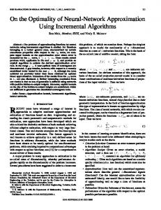
In Tables 1-6, we have shown the outputs of different case orderings against different k, l and c values. We have considered two different k values - 5 and 10, three different l-values – 2, 5, and 10, and two different c values – 2, and 3. Figures 48-51 show the comparison of the percentage of noise nodes added for different case orderings for different l values. The figures clearly show that there is a huge difference in maximum and minimum number of noise nodes added to achieve recursive (c, l) diversity anonymization e.g. if we apply case ordering 312 for k=10, l=10, and c=2, then 21.7% noise nodes will be required to achieve recursive (c, l) diversity anonymization while for the same k, l, and c value, if we apply case ordering 123 or 321, only 10.9% noise nodes will be required which is almost 10% less than the percentage of noise node required for the case ordering 312. Similarly, for different k, l and c values, we have shown that there exists a significant difference in the percentage of


204


noise nodes added for different case orderings. Thus, the results also support our claim that there should be an ordering of the cases of neighborhood edge editing algorithm so that minimal number of noise nodes is added to achieve recursive (c, l) diversity anonymization. In the following two sub-sections, we have discussed the performance of our proposed algorithm against the algorithm proposed in [22].

6.2.1

Noise Node Reduction

In this section, we show the effectiveness of our proposed algorithm in generating an anonymized dataset for a particular set of values of k, l, and c with addition of minimal number of noise nodes. Here, we have compared the percentage of noise nodes added by our proposed method and the existing method given in [22]. The approach in [22] does not use the concept of optimal ordering of the cases in the neighborhood edge editing algorithm, so the raw data can be anonymized using any one of the four case orderings, of which only one is optimal. So, it is expected that the number of noise nodes to be added will be more in comparison to our approach as our approach is based upon the optimal case ordering obtained from the algorithm proposed in section 5.4 and then generates the anonymized graph using that case ordering, so the number of noise nodes added is always minimal i.e. our algorithm detects the best scenario for case ordering which results to minimal number of noise node addition. We have used the following formula to compute the percentage of noise nodes. @Vc9> A+ A;:9 A 9: B 9 100 A;:9 A 9 D9>.9 7B=9 zA7BC @Vc9> A+ A 9: D>9:9 7 ; 789 >Bg =>BD8 In Figures 52-65, the line labeled as Proposed represents the percentage of noise nodes added by using our proposed approach and the line labeled as Existing denotes the percentage of noise nodes to be added by applying the method proposed in [22]. We have considered the worst case scenario of case ordering while computing the number of noise nodes required to be added for the algorithm in [22] in order to highlight the optimal difference between it and our proposed algorithm. The differences in the number of noise nodes to be added signify the efficiency of our approach.





Figure 56: Percentage of noise nodes for different k values (l=8, c=2)

205





206











207


Figures 52-55 denote the percentage of noise nodes required to be added by the two methods to anonymize the raw Prefuse dataset. For the Prefuse dataset, we have considered two different k values; 5 and 10, as the size of the dataset is relatively small. We have measured the performance of both the algorithms for three different l values; 2, 5, 10 and two different c values; 2 and 3. From these figures, we observe that our method produces anonymized data by adding less number of noise nodes and for higher values of k and l, our approach achieves anonymization with almost 10% less number of noise nodes as compared to the method proposed in [22]. Figures 56-61 represent the percentage of noise nodes added by both the methods to anonymize the raw co-authorship data for different k, l and c values respectively. For the co-authorship dataset, we have considered seven different k values, three different l values and two different c values. As the dataset size and the number of sensitive labels are more as compared to the Prefuse dataset, we have considered higher values of k and l for our experimental purpose. For each different combination of k, l and c values, our proposed method produces anonymized graph with lesser number of noise nodes being added. The usage of higher values of k and l also denotes that our proposed method can also be scaled up according to the data size. Figures 62-65 represent the percentage of noise nodes added by both the methods to anonymize the raw Cora dataset for different k, l and c values respectively. For the Cora dataset, we have considered nine different k values along with two different l values and two different c values. As the number of distinct sensitive label is small, we have considered only two different l values but we have considered a very wide range k values, because the dataset is large. For each scenario, our proposed method generates the anonymized graph with lesser number of noise


208


nodes. On average, our method requires 2% less noise nodes to achieve anonymization, which is a huge number for such a large dataset. For some cases, our proposed method requires almost 4-5% less number of noise nodes which is almost equal to 100 noise nodes. So, with the results obtained from the above figures, we can conclude that our proposed method always produces an anonymized graph by adding lesser number of noise nodes. We have also tested our method with very high k and l values to test the scalability of our proposed method. The results clearly indicate that our method scales up perfectly for large data sets and also maintains its effectiveness in producing anonymized data with the addition of minimal number of noise nodes. In the next sub section, we have discussed the utility of the anonymized data obtained from our proposed method.

6.2.2

Data Utility

To analyze the utility of the anonymized data, we have used the precision index [5]. The precision index value can be used to detect the similarities between sets of clusters. Let’s consider a graph consisting of n nodes and m different communities, and each community is assigned sensitive label l, then all the nodes belonging to that community is also assigned sensitive label l. For our experimental purpose, we assume that the sensitive label of the nodes in the original dataset is l. After anonymization, we compute the most frequently occurring sensitive label in each cluster and assign it to all the nodes in the cluster. Let us assume that the most frequently occurring sensitive label is lf. Then, ∑|}, C , C4 ; gℎ9>9, d, X = 1 ;+ d X B d, X = 0, ;+ d s X. >9.;:;A The anonymization algorithm using noise nodes works in an intelligent manner such that, the addition of noise nodes does not affect the sensitive label distribution of the nodes which are already present in the raw graph. Now let’s suppose that ~ and i are the number of noise nodes to be added by our proposed approach and the method proposed in [22] respectively. As we have already shown in the previous section, that our proposed method always adds minimal number of noise nodes, we have ~ - i ; for every case orderings. For any noise node whose sensitive label after anonymization is C , g9 8B D ∗ = C , C4 1

|},

∑|}, ‰ C , C4 D∗ D~ = ………… B + ~ 0 ~ 1 ‹ ∑|}, C , C4 D∗ Di ………… c + i 0 i As ~ - i for all the cases, D~ O Di and also D D~ - D Di . So, the above results show that our proposed approach preserves the utility of the anonymized data better by adding minimal number of noise nodes which ultimately results in less divergence from the raw data.

7

Conclusion and Future work

In this paper, we identified a few deficiencies in the approach proposed in [22] and proposed new algorithms to improve the recursive (c, l) diversity anonymization model for social networks proposed in [22] which uses noise node addition approach for anonymization. We established the necessity of these improvements both theoretically and experimentally and illustrated how these improvements can be utilized to achieve better results. The aim of this paper is to reduce the number of noise nodes added for anonymization as far as practicable. Our proposed algorithms reduce the number of noise nodes required to achieve recursive (c, l) diversity anonymization. This work can be further extended for any other model where the highest degree in that equivalence group is not set as the target degree of the other nodes present in that equivalence group.

References [1] Backstrom, L., Dwork, C., Kleinberg, J.M. (2007) Wherefore Art Thou R3579X?: Anonymized Social Networks, Hidden Patterns, and Structural Steganography, Proceedings of the Sixteenth International World Wide Web conference (WWW2007) 181-190


210


[2] Bhagat, S., Cormode, G., Krishnamurthy, B., Srivastava, D. (2009) Class-Based Graph Anonymization for Social Network Data, Proceedings of VLDB Endowment 2:1 766-777 [3] Campan, A., Truta, T. M. (2008) A Clustering Approach for Data and Structural Anonymity in Social Networks, Proceedings of the Second ACM SIGKDD International Workshop on Privacy, Security, and Trust in KDD (PinKDD’08) [4] Campan, A., Truta, T.M., Cooper, N. (2010) P-Sensitive K-Anonymity with Generalization Constraints, Transactions Data Privacy 3:2 65-89 [5] Casas-Roma, J., Herrera-Joancomarti, J., Torra, V. (2014) Anonymizing Graphs: Measuring Quality for Clustering, Knowledge and Information Systems (KAIS) 1-22 [6] Cheng, J., Fu, A.W.-c., Liu, J. (2010) K-Isomorphism: Privacy Preserving Network Publication against Structural Attacks, Proceedings of International Conference on Management of Data 459-470 [7] Cormode, G., Srivastava, D., Yu, T., Zhang, Q. (2008) Anonymizing Bipartite Graph Data Using Safe Groupings, Proceedings of VLDB Endowment 1:1 833-844 [8] Frikken, K.B., Golle, P. (2006) Private Social Network Analysis: How to Assemble Pieces of a Graph Privately, Proceedings of Fifth ACM Workshop Privacy in Electronic Society (WPES ’06) 89-98 [9] Hay, M., Miklau, G., Jensen, D., Towsley, D., Weis, P. (2008) Resisting Structural Re-Identification in Anonymized Social Networks, Proceedings of VLDB Endowment 1:1 102-114 [10] Heer, J., Card, S.K., Landay, J.A. (2005) Prefuse: a toolkit for interactive information visualization, In Proceedings of the SIGCHI Conference on Human Factors in Computing Systems (CHI '05), ACM New York, NY, USA 421-430 [11] Li, N., Li, T. (2007) t-Closeness: Privacy Beyond k-Anonymity and l-Diversity, Proceedings of IEEE 23rd International Conference on Data Eng. (ICDE’07) 106-115 [12] Liu, K., Terzi, E. (2008) Towards Identity Anonymization on Graphs, SIGMOD’08: Proceedings of ACM SIGMOD International Conference on Management of Data 93-106 [13] Liu, L., Wang, J., Liu, J., Zhang, J. (2008) Privacy Preserving in Social Networks against Sensitive Edge Disclosure, Technical Report CMIDA-HiPSCCS 006-008 [14] Machanavajjhala, A., Kifer, D., Gehrke, J., Venkitasubramaniam, M. (2007) lDiversity: Privacy Beyond k-Anonymity, ACM Transactions on Knowledge Discovery from Data (TKDD) 1:1 [15] Narayanan, A., Shmatikov, V. (2009) De-Anonymizing Social Networks, Proceedings of 30th IEEE Symposium on Security and Privacy (S&P 2009) 173-187



211

[16] Newman, M. E. (2006) Finding community structure in networks using the eigenvectors of matrices, Physical review E, 74:3 [17] Shrivastava, N., Majumder, A., Rastogi, R. (2008) Mining (Social) Network Graphs to Detect Random Link Attacks, Proceedings of IEEE 24th International Conference on Data Engineering (ICDE ’08) 486-495 [18] Stokes, K., Torra, V. (2012) Reidentification and k-anonymity: a model for disclosure risk in graphs, Soft Computing, Springer-Verlag 16:10 1657-1670 [19] Sweeney, L. (2002) k-Anonymity: A Model for Protecting Privacy, International Journal of Uncertainty, Fuzziness and Knowledge-Based Systems 10:5 557-570 [20] Ying, X., Wu, X. (2008) Randomizing Social Networks: A Spectrum Preserving Approach, Proceedings of Eighth SIAM International Conference on Data Mining (SDM ’08) 739-750 [21] Ying, X., Wu, X., Barbara, D. (2011) Spectrum Based Fraud Detection in Social Networks, Proceedings of IEEE 27th International Conference on data engineering (ICDE ’11), Washington DC, IEEE Computer Society, Silver Spring 912-923 [22] Yuan, M., Chen, L., Yu, P.S., Yu, T. (2013) Protecting Sensitive Labels in Social Network Data Anonymization, IEEE Transactions on Knowledge and Data Engineering (TKDE) 25:3 633-647 [23] Zheleva, E., Getoor, L. (2007) Preserving the Privacy of Sensitive Relationships in Graph Data, Proceedings of First ACM SIGKDD International Conference on Privacy, Security, and Trust in KDD (PinKDD ’07) 153-171 [24] Zheleva, E., Getoor, L. (2009) To Join or Not to Join: The Illusion of Privacy in Social Networks with Mixed Public and Private User Profiles, Proceedings of 18th International Conference on World Wide Web (WWW ’09) 531-540 [25] Zhou, B., Pei, J. (2008) Preserving Privacy in Social Networks Against Neighborhood Attacks, Proceedings of IEEE 24th International Conference on Data Engineering (ICDE ’08) 506-515 [26] Zhou, B., Pei, J. (2011) The k-Anonymity and l-Diversity Approaches for Privacy Preservation in Social Networks against Neighborhood Attacks, Knowledge and Information Systems 28:1 47-77 [27] Zou, L., Chen, L., Ozsu, M.T. (2009) K-Automorphism: A General Framework for Privacy Preserving Network Publication, Proceedings of the 35th International Conference on Very Large Databases (VLDB 2009) VLDB Endowment 2:1 946-957


212


Appendix Theorem 1: The minimum number of noise nodes required to be added in the algorithm (Noise node addition to increase degree) is equal to the ceiling of the average degree change required by the nodes which need to increase their degrees and that the minimum number of noise nodes occur only when all those nodes are interconnected (one hop or two hop neighbor of each other). Proof: Let’s say, there are m number of nodes present in a graph which need to increase their degree to achieve the target degree and now there can be two possibilities: 1) All the nodes need to increase their degree by the same amount 2) Some of the nodes or all the nodes need to increase their degree by different amount. Case 1: Let’s first consider the case where all the nodes need to increase their degree by same amount that is all the nodes need to increase their degree by ∈ m . This means that when n will be equal to zero, all the nodes will be achieving their target degrees. Now, for all the m nodes, only the following three cases can be possible: i. All nodes which need to increase degree are connected to each other. ii. Some of the nodes which need to increase their degree are connected with each other. iii. None of the nodes which need to increase their degrees are connected with each other. Scenario i: If all the nodes are inter-connected then after the addition of a single noise node, all the nodes need to increase their degree by 1. Addition of noise nodes will continue until 0. So, the process of increase of degrees of the nodes will correspond to the values of n in the following way until n equals to zero i.e. , − 1, − 2, − 3, … . ,1,0 and as all the nodes are connected, the number of noise nodes will increase in the reverse order 0,1,2, … . . , − 3, − 2, − 1, . So, total noise node addition i.e. , = … … … … … … … … … . . 1 Scenario ii: If some of the nodes are interconnected, then all of them can’t achieve their target degree at the same step. Let’s say 2 of them are not connected to any of the nodes, then for the other − 2 nodes, if they are all inter-connected, n number of noise nodes will be required and for those 2 nodes, extra 2 number of noise nodes will be added. If 3 nodes are not inter-connected, then 3 extra noise nodes will be added. So, total noise nodes for the above two cases are: - 0 2 B 0 3 respectively.



213

So, if we have k number of nodes which are not inter-connected, then, total number of noise nodes, for any k number of nodes 0 h . ∴

0 h

•

…………………………………. 2

As, k can’t be any negative integer, we have, , - • , ∀ h . Case iii: If we further extend the results in Case ii, i.e. for,h V 1 which denotes that none of the nodes are inter-connected, then total number of noise nodes will be, Ž

0 V

So, we can conclude that, • So, the average degrees change

1

V ∗ ………………………. 3 , - Ž ; B: ∈ m, u v .

Ž as h - V and also 3∗ 3

Therefore, Minimum noise nodes will be required when all the nodes are interconnected… … … … … … … 4 . 2) Now, let’s consider that all the m nodes or some of the m nodes need to increase their degree by different amount, but total degree change is M. Two of the following cases can occur 2.1) M is perfectly divisible by m and 2.2) M is not perfectly divisible by m. As in case 1, it has been already proved that minimum number of noise node occurs when all the nodes are inter-connected, so in this case, we have considered only the particular scenario, where all the nodes are connected. So, we have to prove only that the minimum number of noise nodes is equal to the celling of the average degree change. Let’s first consider the case 2.1. As M is perfectly divisible by m, the average obtained will also be an integer. Let’s consider the average is n. Now, the degree increase amount of the nodes can be in the following order: 0 h, , 0 h• , … … , 0 h36, , 0 h3 ; 0 B h1 w h2 w ⋯ w hV 1 w hV 1 0 hV So, the minimum degree change is 0 h3 . As all the nodes are inter-connected, so if we connect 0 h3 noise nodes, the amount of degree increase required by the other :@.8 78B7 h1 0 h2 0 ⋯ 0 hV

nodes will be in the following order: 0 h,

0 h3 ,

0 h•

0 h3 , … … ,

0 h36,

0 h3 , 0

Now, we can see that noise nodes will be added until 0 h, is equal to zero as h, w h• w ⋯ w h36, w h3 . So, to increase the degree by of 0 h, , additional S 0 h, 0 h3 T h, h3 noise nodes will be required. Therefore, total noise nodes required 0 h3 0 h, h3 0 h, . Now, 0 h, will be minimum if h, 0 and B: h, w h• w ⋯ w h36, w h3 B h, 0 h• 0 ⋯ 0 h36, 0 h3 0, so h, , h• , … , h36, , h3 all will be individually zero i.e. the scenario i of case1. Therefore, the minimum number of noise nodes will be equal to , which is equal to the ceiling of the average degree change required by all the nodes.


214


Next consider the case 2.2, where M is not perfectly divisible by m. Let n be the average degree where ∉ m and consider the degree increase amount of the nodes are in the following order: 0 h, , 0 h• , … … , 0 h36, , 0 h3 ; :@.8 78B7 h, w h• w ⋯ w h36, w h3

As all the nodes are inter-connected and minimum degree change is 0 h3 , these many noise nodes are required to be added. The remaining degree increase order can be represented by the sequence: 0 h,

0 h3 ,

0 h•

0 h3 , … … ,

0 h36,

0 h3 ,0

Now, following the procedure in the case 2.1, we can similarly prove that the number of noise nodes added will be 0 h, and this value will be minimal when h, 0. So, minimum number of noise nodes is equal to n but as ∉ m, so number of noise nodes can be either ⌊n⌋ or unv. >, and unv= 0 >• ; where >, 0 >• 1. Let’s say, ⌊n⌋= Now, if we consider, the case, where the nodes need to increase their degree by ⌊n⌋, then maximum m-1 nodes can increase its degree by ⌊n⌋. The m-th node will need to increase its degree by: ’

V

1 ⌊n⌋ ’ V⌊n⌋ ⌊n⌋ ’ V >, ’ V 0 V>, 0 ⌊n⌋ V>, 0 >,

⌊n⌋

As all the nodes are inter-connected, the minimum number of noise nodes added will be equal to the highest degree change i.e. V>, 0 >, as V>, 0 >, O ⌊n⌋+A> ∀ V, >, .

So, here the minimum number of noise nodes to be added is V>, 0 >, … … … … … … … … … … … … . 5

Now, if we consider the case where the increase in the degree of the nodes is unv then maximum m-1 nodes can increase its degree by unv. So, the degree increase required by the m-th node will be: ’ V 1 unv ’ Vunv unv unv ’ V 0 >• ’ V V>• 0 unv 0 >• V>• unv m>•

As all the nodes are inter-connected, therefore, the minimum number of noise nodes added will be equal to the highest degree change i.e. unv because unv > unv m>• So, the minimum number of noise node is unv … … … … … … … … … … … … … … … … … 6 Now, if we rewriting equation 5 in terms of >• , then V>, 0

>,

V 1 >• 0 1 >• V V>• 0 1 0 >• unv 0 V V>• 1



215

⌈nv + V 1 − >• − 1 = ⌈nv + V>, − 1 … … … … … … … … … … … … 7 Now, the value of unv + V>, − 1 is minimum when value of V>, − 1 is minimum. As, V>, ∈ m B V>, O 0 ∀ >, , 7ℎ9 V; ;V@V , 1 ;: “9>A. Therefore, the minimum value of equation 7 is ⌈nv

Therefore, for both case 2.1 and case 2.2, the minimum number of noise node added is unv … … … … . . 8 So, from equations 4 and 8, we can conclude that the minimum number of noise nodes added is equal to the ceiling of the average degree change required by the nodes which need to increase their degree and this occurs only when the nodes are inter-connected. Theorem 2: The maximum number of noise required to be added in the algorithm (Noise node addition to increase degree) is equal to the summation of the degree change required by all the nodes which need to increase their degree to achieve their target degrees. Proof: From case 1 of theorem 1, where all the nodes need to increase their degrees by equal amounts, the maximum number of noise node required is V and this occurs when none of them are inter-connected. Now, we calculate case 2 of theorem 1 i.e. when all or some of the nodes need to change their degrees by different amount and none of them are inter-connected. As it is shown in theorem 1 that maximum number of noise nodes occurs when none of the nodes are inter-connected, so we consider this particular case to compute the maximum number of noise nodes. Let the degree increase amount of the nodes can be in the following order: + h, , + h• , … … , + h36, , + h3 ; :@.ℎ 78B7 h, ≥ h• ≥ ⋯ ≥ h36, ≥ h3

As none of the nodes are inter-connected with each other the total noise node required is: 0 h, 0 0 h• 0. . … … + + h36, + + h3 =

7A7BC @Vc9> A+ 9=>99 ; .>9B:9 >9?@;>9 cX 789 A 9: 7A B.8; >9:D9.7;=97 9=>99.

So, for both the cases the maximum number of noise nodes required to be added is equal to the total degree change required by the nodes which needs to increase their degree to achieve the target degree.


Diversity Anonymization in Social Networks - Transactions on Data ...

Diversity Anonymization in Social Networks - Transactions on Data ...

Suggest Documents

Utility-Oriented K-Anonymization on Social Networks

Utility-Oriented K-Anonymization on Social Networks

Utility-Oriented K-Anonymization on Social Networks - Singapore

Diversity in open social networks

A Detailed Survey on Anonymization Methods of Social Networks

A Detailed Survey on Anonymization Methods of Social Networks

On Anonymization of String Data

On Optimal Anonymization for l -Diversity - CiteSeerX

Quantification of De-anonymization Risks in Social Networks

k-symmetry model for identity anonymization in social networks

(FiM): Tackling De-Anonymization in Social Networks - Semantic Scholar

Anonymization and Uncertainty in Social Network Data - DIMACS

Anonymization and Uncertainty in Social Network Data - dimacs

Protecting Sensitive Labels in Social Network Data Anonymization - Ijltet

Anonymization and Uncertainty in Social Network Data - dimacs

Neural Networks, IEEE Transactions on

Transactions on Networks and Communications

Neural Networks, IEEE Transactions on

Transactions on Networks and Communications

Neural Networks, IEEE Transactions on

Privacy Preservation by k-Anonymization of Weighted Social Networks

k-Anonymization of Social Networks By Vertex Addition

Using Identity Separation Against De-anonymization of Social Networks

Using Identity Separation Against De-anonymization of Social Networks