Diversity Control in Particle Swarm Optimization Shi Cheng∗†
Yuhui Shi†
[email protected] of Electrical Engineering and Electronics University of Liverpool, Liverpool, UK
[email protected] of Electrical & Electronic Engineering Xi’an Jiaotong-Liverpool University, Suzhou, China
∗ Dept.
† Dept.
Abstract—Population diversity of particle swarm optimization (PSO) is important when measuring and dynamically adjusting algorithm’s ability of “exploration” or “exploitation”. Population diversities of PSO based on L1 norm are given in this paper. Useful information on search process of an optimization algorithm could be obtained by using this measurement. Properties of PSO diversity based on L1 norm are discussed. Several methods for diversity control are tested on benchmark functions, and the method based on current position and average of current velocities has the best performance. This method could control the PSO diversity effectively and gets better performance than the standard PSO.
I. I NTRODUCTION Particle Swarm Optimization (PSO), which is one of the evolutionary computation techniques, was invented by Russ Eberhart and James Kennedy in 1995 [1], [2]. It is a populationbased stochastic algorithm modeled on the social behaviors observed in flocking birds. Each particle, which represents a solution, flies through the search space with a velocity that is dynamically adjusted according to its own and its companion’s historical behaviors. The particles tend to fly toward better search areas over the course of the search process [3], [4]. In this paper, the basic PSO algorithm and the importance of diversity will be reviewed in Section II. In Section III, a comparison of element-wise PSO diversity and dimensionwise PSO diversity, which based on L1 norm or L2 norm are given, followed by experiments on diversity monitoring and analysis for some benchmark functions in Section IV. Several methods for diversity control are tested on benchmark functions in Section V, and a novel method based on current position and average of current velocities has the best performance. Finally, Section VI concludes with some remarks and future research directions. II. PARTICLE S WARM O PTIMIZATION The original PSO algorithm is simple in concept and easy in implementation [5], [6]. The basic equations are as follow: vij = vij + c1 rand()(pij − xij ) + c2 Rand()(pnj − xij ) xij = xij + vij
(1) (2)
where c1 and c2 are positive constants, and rand() and Rand() are two random functions in the range [0, 1] and are different for each dimension and each particle.
978-1-61284-052-9/11/$26.00 ©2011 IEEE
The most important factor affecting an optimization algorithm’s performance is its ability of “exploration” or “exploitation”. Exploration means the ability of a search algorithm to explore different areas of the search space in order to have high probability finding good optimum. Exploitation, on the other hand, means the ability to concentrate the search around a promising region in order to refine a candidate solution. A good optimization algorithm optimally balances these conflicted objectives. Within the PSO, these objectives are addressed by the velocity update equation. Velocity clamp was firstly used to adjust the ability between exploration and exploitation [7]. Like the equation below, current velocity will be equal to maximum velocity or minus maximum velocity if velocity is greater than the maximum velocity or less than the minus maximum velocity, respectively. vij > Vmax Vmax vij −Vmax ≤ vij ≤ Vmax (3) vij = −Vmax vij < −Vmax However, velocity clamp only makes algorithm less like to diverge, it cannot help algorithm “jump out” a local optimum or refine the candidate solution. Shi and Eberhart introduced a new parameter, an inertia weight w to balance the exploration and exploitation [8] [9]. This inertia weight w is added to equation (1), and it can be a constant, linear decreasing value over time [10], or fuzzy value [11], [12]. The new velocity update equation is as follows: vij = wvij + c1 rand()(pij − xij ) + c2 Rand()(pnj − xij )
(4)
Adding an inertia weight is more effective than velocity clamp for it is not only increasing the probability for algorithm to converge, but have a way to control the whole process of algorithm’s searching. Generally speaking, algorithm should have a bigger exploration and lower exploitation ability at first, which has a high probability to find more local optima. Exploration should be decreased, and exploitation should be increased to refine candidate solutions over the time. Accordingly, the inertia weight w, should be linear decreased or even dynamically determined by a fuzzy system. The whole process of PSO search could be adjusted by adding an inertia weight, however, it is difficult to change inertia weight in order to dynamically adjust the ability of exploration or exploitation during algorithm searching. Diversity, which can be a way to monitor an algorithm’s state of
exploration or exploitation, is important for helping adjust the ability of exploration and exploitation. Diversity can reveal internal characteristic of a search process.
Dimension-wise definition [15] is as follows: 1 ∑ xij m i=1 v um u∑ 1 p ¯j )2 D = t (xij − x m i=1 m
¯= x
III. D IVERSITY D EFINITION Population diversity is a way to monitor the degree of convergence or divergence in PSO search process [13], [14]. In other words, the particles’ current distribution and velocity tendency, whether it is in the state of “fly” to a large search space or refine in a local area, can be obtained from this measurement. Shi and Eberhart gave several definitions of PSO population diversity measurements in [15], [16], [17], and these definitions of population diversities could be divided into three parts: position diversity, velocity diversity, and cognitive diversity. The analysis of different definitions is as follows. A. Position Diversity Position diversity measures distribution of particles’ current positions whether the particles are going to diverge or converge could be reflected from this measurement. Position diversity gives the current distribution information of particles. Position diversity could be measured either element-wise or dimension-wise. For the purpose of generality and clarity, m represents the number of particles and n the number of dimensions. Each particle is represented as xij , i represents the ith particle, i = 1, · · · , m, and j is the jth dimension, j = 1, · · · , n. Element-wise definition [15] is as follows: 1 ∑∑ xij m × n i=1 j=1
(5)
1 ∑∑ (xij − x ¯ )2 m × n i=1 j=1
(6)
m
x ¯=
m
p DE =
n
n
where x ¯ is the mean of current position for all particles in all p dimensions, and DE measures all particles position diversity in all dimensions. Element-wise measurement sets all particles and all dimensions as an entirety to calculate the population diversity of PSO, therefore, this kind of definitions has some blemishes: •
•
p Lack of each dimension’s diversity information: DE represents the swarm position diversity, no measurement of particles’ position diversity on a single dimension. Confusion about the difference in dimensions: Consider a simple scenario, using two particles to solve a problem with two dimensions, particles at (1, 7) and (7, 1), respectively; or two particles converge to (1, 7), the results of element-wise diversity are same: x ¯ = 4, p DE = 9. However, these two situations should have different results of population diversity measurement. The above example shows that element-wise diversity cannot give the useful information of problem’s optimum with different values among all dimensions.
(7)
(8)
¯ = [¯ ¯ represents the mean where x x1 , · · · , x ¯j , · · · , x ¯n ], x of particles’ current positions on each dimension. Dp = [D1p , · · · , Djp , · · · , Dnp ], which measures particles’ position diversity based on L2 norm for each dimension, therefore, it lacks of whole swarm information during algorithm search process. Furthermore, L1 norm can be used to instead of L2 norm. New definition of position diversity, which based on the L1 norm, is as follows: 1 ∑ xij m i=1 m
¯= x
(9)
Dp =
1 ∑ |xij − x ¯j | m i=1
(10)
Dp =
1∑ p D n j=1 j
(11)
m
n
¯ represents the mean ¯ = [¯ ¯j , · · · , x ¯n ], x where x x1 , · · · , x of particles’ current positions on each dimension. Dp = [D1p , · · · , Djp , · · · , Dnp ], which measures particles’ position diversity based on L1 norm for each dimension. Dp measures the whole swarm population diversity. Besides, the definition of diversity on dimensions has clearer ¯ is the center of all positions on each geometric means: x dimension, and Djp is the average distance of particles from the center in j dimension. In other word, if swarm moves to the center from current distribution, the distance of all particles need ∑ to move is mDjp in dimension j, and the total distance n is m j=1 Djp = m × n × Dp = mnDp .
B. Velocity Diversity Velocity diversity, which gives the dynamic information of particles, measures the distribution of particles’ current velocities, In other words, velocity diversity measures the “activity” information of particles. Based on the measurement of velocity diversity, particle’s tendency of expansion or convergence could be revealed. The dimension-wise definition of velocity diversity, which was given by Shi and Eberhart [16], is based on L2 norm.
These velocity diversity definitions are as follow.
PSO cognitive diversity is as follows: 1 ∑ pij m i=1 m
nor vij
vij = √∑ n j=1
v¯jnor =
1 m
m ∑
(12) 2 vij
nor vij
i=1 v um 1 u∑ nor Dv = t (vij − v¯jnor )2 m i=1
(13)
Dcj
1∑ c D = D n j=1 j
(19)
n
c
(14)
1 ∑ vij m i=1
(15)
1 ∑ Dv = |vij − v¯j | m i=1
(16)
1∑ v D D = n j=1 j
(17)
m
(20)
¯ represents the average ¯ = [¯ where p p1 , · · · , p¯j , · · · , p¯n ] and p of all particles’ personal best position in history (pbest) on each dimension; Dc = [D1p , · · · , Djp , · · · , Dnp ], which represents the particles’ cognitive diversity for each dimension based on L1 norm. Dc measures the whole swarm cognitive diversity. The above discussion gives the definitions of population diversities from three parts: position, velocity, and cognitive. These diversity definitions are based on L1 norm which have clearer geometric meaning. Three definitions have the same form and easy to understood or implemented. More searching information of optimization algorithms could be revealed from this measurement. IV. D IVERSITY M ONITORING AND A NALYSIS
m
n
v
1 ∑ = |pij − p¯j | m i=1
(18)
m
where Dv = [D1v , · · · , Djv , · · · , Dnv ], Dv measures velocity diversity based on L2 norm for each single dimension. Similar with definitions of position diversity, velocity diversity based on L2 norm lacks of measurement on whole swarm velocity, Dv only measures velocity distribution on each dimension. L1 norm can also be used to replace L2 norm. New definition of velocity diversity based on L1 norm is as follows:
¯= v
¯= p
¯ = [¯ ¯ represents the mean of where v v1 , · · · , v¯j , · · · , v¯n ], v particles’ current velocities on each dimension; and Dv = [D1v , · · · , Djv , · · · , Dnv ], Dv measures velocity diversity of all particles on each dimension. Dv represents the whole swarm velocity diversity based on L1 norm. In addition, velocity diversity based on L1 norm has clearer ¯ , which is the average velocity of partigeometric meaning: x cles on each dimension, was found at first; then the variance of velocity on each dimension j could be calculated. This variance gives the information of particles “vitality”, even the swarm may have same average of velocity on each dimension during different searching period, the variance will be small when the swarm converges.
C. Cognitive Diversity Cognitive diversity represents the distribution of all current moving targets found by particles. The measurement of cognitive diversity is the same as position diversity except for using each particle’s current personal best position instead of current position. Therefore, the analysis for position diversity is also being applied to cognitive diversity. The diversity could be dimension-wise and based on the L1 norm. The definition of
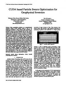
Wolpert and Macerady have proved that under certain assumptions no algorithm is better than other one on average for all problems [18]. Consider the generalization, twelve benchmark functions were used in our experimental studies [19],[20]. The aim of the experiment is not compare the ability or the efficacy of PSO algorithm with different parameter setting or structure, e.g., global star or local ring, but to compare the measurement of runtime information when PSOs are executed. The 12 benchmark functions are given in Table I. Functions f1 − f5 are unimodal. f5 is a noisy quadric function, where random[0, 1) is a uniformly distributed random variable in [0, 1). Functions f6 − f12 are multimodal. f6 has 2 minima when dimensions n = 4 ∼ 30. [21] In all experiments, PSO has 50 particles, and parameters are set as the standard PSO [22]. Each algorithm runs 50 times, 10 000 iterations in each run. Due to the limit of space, the simulation results of three representative benchmark functions are reported here. The functions include f5 , which is a unimodal function with random noise; f9 , which is a noncontinuous multimodal function, and f11 , a continuous multimodal function. A. Comparison of Different PSO Diversity Definitions Figure 1 shows a comparison of different PSO population diversity definitions. Firstly, for the PSO with global star structure, Fig.1 (a) shows the cognitive diversity of f5 function, Fig.1 (b) shows the position diversity of f9 function, and Fig.1 (c) shows the velocity diversity of f11 function; secondly, for the PSO with local ring structure, Fig.1 (d) shows the velocity diversity of f5 function, Fig.1 (e) shows the cognitive diversity
TABLE I BENCHMARK FUNCTIONS USED IN OUR EXPERIMENTAL STUDY, WHERE n IS THE DIMENSION OF THE FUNCTION , fmin IS THE MINIMUM VALUE OF THE FUNCTION , AND S EARCH SPACE ⊆ Rn
T HE 12
Function name Sphere [19] Schwefel’s P2.22 [19] Schwefel’s P1.2 [19] Step [19] Quadric Noise [19] Generalized Rosenbrock [19] Schwefel [19] Generalized Rastrigin [19] Noncontinuous Rastrgin [20]
Ackley [19]
Test function ∑ 2 f1 (x) = n i=1 xi ∑n ∏ f2 (x) = i=1 |xi | + n i=1 |xi | ∑n ∑i f3 (x) = i=1 ( k=1 xk )2 ∑ f4 (x) = n (⌊xi + 0.5⌋)2 ∑i=1 n f5 (x) = i=1 ix4i + random[0, 1) ∑ 2 2 2 f6 (x) = n i=1 [100(xi+1 − xi ) + (xi − 1) ] √ ∑n f7 (x) = i=1 −xi sin( |xi |) + 418.9829n ∑ 2 f8 (x) = n i=1 [xi − 10 cos(2πxi ) + 10] ∑ 2 f9 (x) = n i=1 [yi − 10 cos(2πyi ) + 10] { xi |xi | < 21 yi = round(2xi ) |x | ≥ 1 2 √ i1 ∑n 2 2 f10 (x) = −20e−0.2 n i=1 xi
Dimension 50 50 50 50 50
Search space [−100, 100]n [−10, 10]n [−100, 100]n [−100, 100]n [−1.28, 1.28]n
fmin 0 0 0 0 0
50
[−10, 10]n
0
50
[−500, 500]n
50
[−5.12, 5.12]
0
50
[−5.12, 5.12]n
0
[−32, 32]n
0
[−600, 600]n
0
[−50, 50]n
0
50 1 ∑n −e n i=1 cos(2πxi ) + 20 + e ∏n ∑n x 2 1 √i f11 (x) = 4000 50 i=1 cos( i ) + 1 i=1 xi − ∑ n−1 2 2 π f12 (x) = n {10 sin (πy1 ) + i=1 (yi − 1) 50 ×[1 + 10 sin2 (πyi+1 )] + (yn − 1)2 } ∑n + i=1 u(xi , 10, 100, 4) yi = 1 + 14 (xi + 1) k(xi − a)m xi > a, 0 −a < xi < a u(xi , a, k, m) = k(−x − a)m xi < −a i
Griewank [19] Generalized Penalized [19]
0
2
10
0
n
4
10
10 dimension−wise L1 element−wise dimension−wise L
2
10 2
1
10
0
10 −1
10
−2
10 0
10
−4
10 −2
L1 norm
10
−6
10
−1
L2 norm
10 dimension−wise L1
−8
10
element−wise dimension−wise L2 −3
−2
10
−10
10 0
1
10
10
2
10
3
10
4
10 0
10
10
1
2
10
(a)
10
3
10
4
0
10
10
1
2
10
(b)
10
3
10
4
10
(c)
0
6
10
10
5
10 −1
4
10
10
3
10 −2
2
10
10 dimension−wise L1 0
10
1
element−wise dimension−wise L2
10
−3
0
10
10
dimension−wise L1 L norm
−1
10
1
element−wise dimension−wise L2
L2 norm −4
−2
10
10 0
10
1
10
2
10
(d)
3
10
4
10
0
10
1
10
2
10
(e)
3
10
4
10
0
10
1
10
2
10
3
10
4
10
(f)
Fig. 1. Different definitions of PSO population diversity. Global star structure: (a) f5 cognitive, (b) f9 Position, (c) f11 velocity; Local ring structure: (d) f5 velocity, (e) f9 cognitive, (f) f11 position
of f9 function, and Fig.1 (f) shows the position diversity of f11 function. From the Figure 1, conclusions could be made that dimension-wise population diversities is better than elementwise. The measurement of element-wise diversity cannot give useful information of particles’ distribution. The diversity based on L1 norm and L2 norm have the same changing curve. L1 norm is better than L2 norm for two reasons: • •
In general terms, L1 norm have higher computational efficiency. The value of L1 is larger than L2 norm, (Figure 1: (a), (b), (e), (f)), or the value of L1 has larger variation range (Figure 1: (c), (d)). These show that diversity based on L1 norm can reveal more significant information at least for the tested benchmark functions under dimension-wise population diversity.
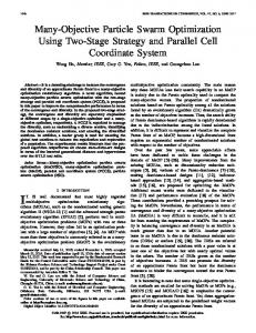
B. PSO Diversity Analysis Figure 2 displays the population diversities which includes position diversity, cognitive diversity, and velocity diversity. Firstly, Fig.2 (a), (b), (c) display the diversities of f5 function, f9 function, and f11 function for PSO with global star structure, respectively; secondly, Fig.2 (d), (e), (f) display the diversities of f5 function, f9 function, and f11 function for PSO with local ring structure, respectively. From the figure, some conclusions could be made that position diversity and cognitive diversity have the same changing tendency, and cognitive diversity curve is a simplified position diversity curve without vibrate. Velocity diversity will fall to a tiny value after algorithm find a “good enough” value or “stuck” in a local optimum. It is observed from running PSO that particles “fly” from one side of optimum to another side on each dimension continually [23]. Velocity diversity and position diversity usually have a continuous vibrate. V. D IVERSITY C ONTROL Diversity is the measurement of exploration and exploitation, however, the goal is not only to observe, but to control the diversity, that is state of the exploration or exploitation could be dynamically adjusted. Since adding random noise may increases population diversity, in the first experiment below, we add noise in PSO to see its impacts. A. Based on Random Noise Noise is added to equation (2), new equation is as follows: xij = xij + vij + c3 RAND()
(21)
where c3 could be a positive or negative constant, or adjusted during the algorithm search process. RAND() is a random function in the range [0, 1] and the value is different for each dimension and each particle. Some representative results are given in Table II. This method does not performs better than the standard PSO.
B. Based on Average of Current Velocities Velocity measures the “flying” tendency of particles. The average of current velocities may affect the population diversity. The next experiment, which adds the average velocity to equitation (2), is as follows: xij = xij + vij + c3 RAND()¯ vj
(22)
where c3 could be a positive or negative constant, or adjusted during the algorithm search process. RAND() is a random function in the range [0, 1] and the value is different for each dimension and each particle; v¯j is the average of current velocities for dimension j. Some representative results are shown in table III. This method does not have significant improvement over the standard PSO. C. Based on Current Position and Average of Current Velocities In the third experiment, we utilize current position in addition to the current average velocity. The new equation is as follows: xij = xij + vij + c3 RAND()(xij − v¯j )
(23)
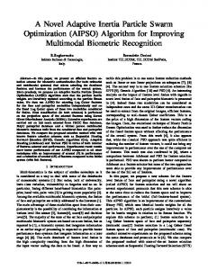
where c3 could be a positive or negative constant, or adjusted during the algorithm searching. RAND() is a random function in the range [0, 1] and is different for each dimension and each particle; v¯j is the average of current velocities for dimension j. Several representative results are shown in table IV. Some significant improvements are achieved from this method, the best or mean of results are much better than the standard PSO. Figure 3 measures the difference of the standard PSO and PSO with diversity control: firstly, for the PSO with global star structure, Fig.3 (a) shows the position diversity of f5 function, Fig.3 (b) shows the cognitive diversity of f9 function, and Fig.3 (c) shows the velocity diversity of f11 function; secondly, for the PSO with local ring structure, Fig.3 (d) shows the cognitive diversity of f5 function, Fig.3 (e) shows the velocity diversity of f9 , and Fig.3 (f) shows the position diversity of f11 function. From the Table IV and Figure 3, conclusions could be made that if c3 is positive, the diversity will be increased, particles search wider area than the standard PSO does, the results have a large variance. If c3 is negative, the diversity will be decreased, particles converge faster than the standard PSO, the results have a small variance. If c3 was initialized with a positive value and decreases to negative values during PSO search process, both the best and mean result will be improved. The relationship between this new parameter and diversity control is still required to be further researched. How to set this parameter c3 , or how to adjust this parameter for different problem during different state of PSO searching is our future work.
0
1
10
4
10
10
2
10
0
10 −1
0
10
10
−2
10
−4
10 −2
−1
10
10
−6
10 cognitive position velocity
cognitive position velocity
−3
−2
10
−10
10 0
10
1
10
2
3
10
10
4
10 0
10
cognitive position velocity
−8
10
10
1
10
(a)
2
10
3
4
10
0
10
10
1
10
(b)
2
10
3
10
4
10
(c)
0
50
10
10
0
10
−50
10 −1
cognitive position velocity
0
10
10
−100
10
−150
10 −2
cognitive position velocity
−200
10
10
−250
10
cognitive position velocity
−300
10
−3
10
0
10
1
10
2
10
3
10
4
10
0
10
1
10
(d)
2
10
(e)
3
10
4
10
0
10
1
10
2
10
3
10
4
10
(f)
Fig. 2. PSO population diversity analysis. Global star structure: (a) f5 population, (b) f9 population, (c) f11 population; Local ring structure: (d) f5 population, (e) f9 population, (f) f11 population
VI. C ONCLUSION This paper proposed a definition of population diversity based on L1 norm, compared the difference between these different definitions of population diversities, discussed the blemishes of existing definitions, and then analyzed population diversities changing during the algorithm search process. Based on above analysis, a novel position update equation to modify the diversity during PSO search process is presented. New equation has an extra parameter c3 , the diversity could be increased or decreased by setting c3 to be a positive or negative value, respectively. The idea of diversity measuring and controlling can also be applied to other evolutionary algorithms, e.g., genetic algorithm, differential evolution. Because evolutionary algorithms have the same concepts of current population solutions, the position diversity could be measured and adjusted. It can be beneficial to dynamically adjust the algorithm’s ability of exploration or exploitation, especially when the problem to be solved is a difficult or large-scale problem. ACKNOWLEDGMENT The authors’ work is supported by National Natural Science Foundation of China under grant 60975080, and Suzhou Science and Technology Project under Grant SYJG0919. R EFERENCES [1] R. Eberhart and J. Kennedy. A new optimizer using particle swarm theory. In Processings of the Sixth International Symposium on Micro Machine and Human Science, pages 39–43, 1995.
[2] J. Kennedy and R. Eberhart. Particle swarm optimization. In Processings of IEEE International Conference on Neural Networks (ICNN), pages 1942–1948, 1995. [3] R. Eberhart and Y. Shi. Particle swarm optimization: Developments, applications and resources. In Proceedings of the 2001 Congress on Evolutionary Computation (CEC2001), pages 81–86, 2001. [4] X. Hu, Y. Shi, and R. Eberhart. Recent advances in particle swarm. In Proceedings of the 2004 Congress on Evolutionary Computation (CEC2004), pages 90–97, 2004. [5] J. Kennedy, R. Eberhart, and Y. Shi. Swarm Intelligence. Morgan Kaufmann Publisher, first edition, 2001. [6] R. Eberhart and Y. Shi. Computational Intelligence: Concepts to Implementations. Morgan Kaufmann Publisher, first edition, 2007. [7] R. Eberhart, R. Dobbins, and P. Simpson. Computational Intelligence PC Tools. Academic Press Professional, first edition, 1996. [8] Y. Shi and R. Eberhart. Parameter selection in particle swarm optimization. In Proceedings of the 1998 Annual Conference on Evolutionary Computation, pages 591–600, 1998. [9] Y. Shi and R. Eberhart. A modified particle swarm optimizer. In Proceedings of the 1998 Congress on Evolutionary Computation (CEC1998), pages 69–73, 1998. [10] Y. Shi and R. Eberhart. Empirical study of particle swarm optimization. In Proceedings of the 1999 Congress on Evolutionary Computation (CEC1999), pages 1945–1950, 1999. [11] Y. Shi, R. Eberhart, and Y. Chen. Implementation of evolutionary fuzzy system. IEEE Transactions on Fuzzy Systems, 7(2):109–119, 1999. [12] Y. Shi and R. Eberhart. Fuzzy adaptive particle swarm optimization. In Proceedings of the 2001 Congress on Evolutionary Computation (CEC2001), pages 101–106, 2001. [13] M. Clerc and J. Kennedy. The particle swarm–explosion, stability, and convergence in a multidimensional complex space. IEEE Transactions on Evolutionary Computation, 6(1):58–73, February 2002. [14] Z. Zhan, J. Zhang, Y. Li, and H. Chung. Adaptive particle swarm optimization. IEEE Transactions on Systems, Man, and Cybernetics– Part B: Cybernetics, 139(6):1362–1381, December 2009. [15] Y. Shi and R. Eberhart. Population diversity of particle swarms.
0
1
10
10
−1
10
0
10
−2
10
−1
10 −3
10
c3 = −0.4
c3 = −0.4
standard PSO c3 = 0.4 ∼ −0.4
standard PSO c3 = 0.4 ∼ −0.4
c3 = 0.4
c3 = 0.4
−4
−2
10
10 0
10
1
10
2
10
3
10
4
0
10
10
1
10
(a)
2
10
3
10
4
10
(b)
4
0
10
10
2
10
0
10
c3 = −0.4
−2
10
standard PSO c = 0.4 ∼ −0.4
−1
10
3
−4
10
c = 0.4 3
−6
10
c = −0.4 3
standard PSO c3 = 0.4 ∼ −0.4
−8
10
c = 0.4 3
−10
−2
10
10 0
10
1
10
2
10
3
10
4
0
10
10
1
10
(c)
2
10
3
10
4
10
(d) 4
10 0.2
10
2
10 0
10
0
10 −0.2
10
−2
10 −0.4
10
−4
10 c3 = −0.4
−0.6
10
c3 = −0.4
standard PSO c3 = 0.4 ∼ −0.4 −0.8
standard PSO c3 = 0.4 ∼ −0.4
−6
10
c3 = 0.4
10
c3 = 0.4 −8
10 0
10
1
10
2
10
(e)
3
10
4
10
0
10
1
10
2
10
3
10
4
10
(f)
Fig. 3. PSO population diversity control based on current position and average of current velocities. Global star structure: (a) f5 position, (b) f9 cognitive, (c) f11 velocity; Local ring structure: (d) f5 cognitive, (e) f9 velocity, (f) f11 position
TABLE II R EPRESENTATIVE RESULTS OF PSO WITH DIVERSITY CONTROL BASED ON RANDOM NOISE . A LL ALGORITHMS HAVE BEEN RUN OVER 50 TIMES , WHERE “ MEAN ” INDICATES THE MEAN BEST FUNCTION VALUES FOUND IN THE LAST GENERATION .[−0.05, 0.05] INDICATES THAT c3 RAN D() IN THE RANGE OF −0.05 TO 0.05 DURING PSO SEARCH PROCESS
Result Standard PSO [0, 0.05] [0, 0.1] [−0.05, 0] [−0.1, 0] [−0.05, 0.05] [−0.1, 0.1]
best mean best mean best mean best mean best mean best mean best mean
Global star structure f5 f9 f11 0.003306 98.0000 0 3.763743 170.2000 18.0558 0.027495 151.4569 0.001945 3.324122 193.7475 14.4905 0.192631 171.7475 0.006434 5.108825 243.0230 3.639894 0.030778 125.2904 0.001924 2.465845 177.0750 7.250727 0.199754 162.2819 0.007742 6.448594 242.4670 5.450799 0.092398 187.5481 0.006408 0.206316 237.1176 0.022319 0.914132 248.5174 0.023818 1.488689 328.5418 0.046167
Local ring structure f5 f9 f11 0.021183 139.2511 9.7699E-15 0.078473 181.7243 1.7852E-14 0.062837 139.5583 0.002694 0.092465 189.9442 0.003257 0.251453 162.0773 0.008715 0.389412 212.5552 0.012889 0.055127 135.7548 0.002388 0.089502 188.1026 0.003799 0.320260 193.1383 0.010421 0.400614 222.3157 0.012960 0.203883 155.0355 0.007811 0.283535 197.6311 0.010637 1.022184 216.1435 0.027316 1.777710 279.9250 0.041168
TABLE III R EPRESENTATIVE RESULTS OF PSO WITH DIVERSITY CONTROL BASED ON AVERAGE OF CURRENT VELOCITIES . A LL ALGORITHMS HAVE BEEN RUN OVER 50 TIMES , WHERE “ MEAN ” INDICATES THE MEAN BEST FUNCTION VALUES FOUND IN THE LAST GENERATION . c3 ∼ [−0.05, 0.05] INDICATES THAT c3 LINEAR INCREASES FROM −0.05 TO 0.05 DURING PSO SEARCH PROCESS
Result Standard PSO c3 = 0.05 c3 = 0.1 c3 = −0.05 c3 = −0.1 c3 ∼ [−0.05, 0.05] c3 ∼ [−0.1, 0.1]
[16] [17]
[18]
[19]
[20]
[21] [22]
best mean best mean best mean best mean best mean best mean best mean
Global star structure f5 f9 f11 0.003306 98.0000 0 3.763743 170.2000 18.0558 0.000300 91.2810 0 4.835266 154.0616 21.7101 0.000213 51.3985 0 3.653916 139.9491 21.7121 0.000314 83.1481 0 3.976869 144.6972 16.3120 0.000209 66.5491 0 1.990022 153.8094 18.0800 0.000113 65.2646 0 3.707627 153.0410 14.4772 0.000420 90.0021 0 2.365738 165.4357 14.4980
In Proceedings of the 2008 Congress on Evolutionary Computation (CEC2008), pages 1063–1067, 2008. Y. Shi and R. Eberhart. Monitoring of particle swarm optimization. Frontiers of Computer Science, 3(1):31–37, March 2009. Z. Zhan, J. Zhang, and Y. Shi. Experimental study on pso diversity. In Third International Workshop on Advanced Computational Intelligence, pages 310–317, Suzhou Jiangsu, China, August 25–27 2010. D. Wolpert and W. Macready. No free lunch theorems for optimization. IEEE Transactions on Evolutionary Computation, 1(1):67–82, April 1997. X. Yao, Y. Liu, and G. Lin. Evolutionary programming made faster. IEEE Transactions on Evolutionary Computation, 3(2):82–102, July 1999. J. Liang, A. Qin, P. Suganthan, and S. Baskar. Comprehensive learning particle swarm optimizer for global optimization of multimodal functions. IEEE Transactions on Evolutionary Computation, 10(3):281–295, June 2006. Y. Shang and Y. Qiu. A note on the extended rosenbrock function. Evolutionary Computation, 14(1):119–126, 2006. D. Bratton and J. Kennedy. Defining a standard for particle swarm optimization. In Proceedings of the 2007 IEEE Swarm Intelligence Symposium (SIS 2007), pages 120–127, 2007.
Local ring structure f5 f9 f11 0.021183 139.2511 9.7699E-15 0.078473 181.7243 1.7852E-14 0.010046 120.4208 8.8817E-16 0.028780 162.1770 0.000177 0.008539 138.2817 7.7715E-16 0.028096 181.1114 6.4194E-05 0.008869 125.3705 1.4432E-15 0.030871 182.1733 3.2111E-05 0.007992 144.7393 8.8817E-16 0.027247 180.8293 9.6985E-05 0.009003 146.1426 2.3314E-15 0.032105 180.4098 0.000148 0.007660 144.0002 9.9920E-16 0.034546 174.4129 0.000149
[23] W. Spears, D. Green, and D. Spears. Biases in particle swarm optimization. International Journal of Swarm Intenlligence Research, 1(2):34–57, April–June 2010.
TABLE IV R EPRESENTATIVE RESULTS OF PSO WITH DIVERSITY CONTROL BASED ON CURRENT POSITION AND AVERAGE OF CURRENT VELOCITIES . A LL ALGORITHMS HAVE BEEN RUN OVER 50 TIMES , WHERE “ MEAN ” INDICATES THE MEAN BEST FUNCTION VALUES FOUND IN THE LAST GENERATION . c3 ∼ [0.05, −0.05] INDICATES THAT c3 LINEAR DECREASES FROM 0.05 TO −0.05 DURING PSO SEARCH PROCESS
Result Standard PSO c3 = 0.4 c3 = 0.2 c3 = 0.1 c3 = 0.05 c3 = −0.05 c3 = −0.1 c3 = −0.2 c3 = −0.4 c3 = −0.8 c3 = 0.05 ∼ −0.05 c3 = 0.1 ∼ −0.1 c3 = 0.2 ∼ −0.2 c3 = 0.4 ∼ −0.4 c3 = 0.8 ∼ −0.8
best mean best mean best mean best mean best mean best mean best mean best mean best mean best mean best mean best mean best mean best mean best mean
Global star structure f5 f9 f11 0.003306 98.0000 0 3.763743 170.2000 18.0558 15.0484 502.3478 156.2566 44.2900 533.4721 233.7385 0.019737 377.3507 0.000415 15.8242 413.9585 54.3862 0.001361 210.4438 0 7.681045 272.0944 52.3284 0.001999 132.0845 0 8.593309 195.9888 54.2096 9.2408E-05 27.1167 0 0.001132 62.5534 0.005293 3.8991E-05 36.2792 0 0.000707 83.3589 0.004473 1.9932E-05 28.0569 0 0.000549 59.0719 0.004092 5.1783E-05 15.2198 0 0.000358 37.4257 0.003220 0.070678 347.6730 0.022260 2.289617 392.8169 42.3895 0.000418 32.5417 0 0.002872 82.3480 0.012007 0.000453 19.3198 0 0.002000 60.7679 0.012391 0.000216 21.2966 0 0.001909 124.3974 0.009576 4.7276E-05 84.0947 0 0.001344 187.7145 0.012821 1.1010E-06 247.4993 0 0.001127 307.9561 0.001575
Local ring structure f5 f9 f11 0.021183 139.2511 9.7699E-15 0.078473 181.7243 1.7852E-14 10.8490 474.6455 105.0195 26.8031 550.2269 183.7515 0.015253 366.2699 0.166868 0.029428 390.5112 0.416948 0.006296 247.5167 0 0.013490 272.3373 0.000193 0.012057 163.8312 0 0.020866 194.9040 0.000201 0.000468 99.77662 0 0.002397 134.5600 2.2764E-06 3.0822E-05 90.1938 0 0.000527 117.1118 8.8288E-06 8.8024E-06 75.1486 0 0.000486 102.8416 0 4.0767E-06 84.2474 0 0.000362 102.2737 0 0.006103 324.0427 0 0.029982 358.4001 0.213375 0.002921 153.0000 0 0.012222 185.6194 0.000347 0.002940 137.6087 0 0.007120 192.0868 1.2374E-06 0.001008 159.4919 0 0.003633 184.7151 3.0085E-06 0.001177 180.9459 0 0.001970 255.3435 1.9579E-05 7.3074E-05 258.3948 0 0.001389 320.8334 0.000225