arXiv:1603.05691v1 [stat.ML] 17 Mar 2016
Do Deep Convolutional Nets Really Need to be Deep (Or Even Convolutional)? Gregor Urban1 , Krzysztof J. Geras2 , Samira Ebrahimi Kahou3 , Ozlem Aslan4 , Shengjie Wang5 , Rich Caruana6 , Abdelrahman Mohamed6 , Matthai Philipose6 & Matt Richardson6 1 University of California Irvine, USA –
[email protected] 2 University of Edinburgh, UK –
[email protected] 3 Ecole Polytechnique de Montreal, CA –
[email protected] 4 University of Alberta, CA –
[email protected] 5 University of Washington, USA –
[email protected] 6 Microsoft Research, Redmond, USA – {rcaruana, asamir, matthaip, mattri}@microsoft.com
Abstract Yes, apparently they do. Previous research demonstrated that shallow feed-forward nets sometimes can learn the complex functions previously learned by deep nets while using a similar number of parameters as the deep models they mimic. In this paper we investigate if shallow models can learn to mimic the functions learned by deep convolutional models. We experiment with shallow models and models with a varying number of convolutional layers, all trained to mimic a state-of-the-art ensemble of CIFAR10 models. We demonstrate that we are unable to train shallow models to be of comparable accuracy to deep convolutional models. Although the student models do not have to be as deep as the teacher models they mimic, the student models apparently need multiple convolutional layers to learn functions of comparable accuracy.
1. Introduction There is well-known early theoretical work on the representational capacity of neural nets. For example, Cybenko (1989) proved that a network with a large enough single hidden layer of sigmoid units can approximate any decision boundary. Empirical work, however, suggests that it can be difficult to train shallow nets to be as accurate as deep nets. Dauphin and Bengio (2013) trained shallow nets on SIFT features to classify a large-scale ImageNet dataset and found that it was difficult to train large, high-accuracy, shallow nets. A study of deep convolutional nets suggests that for vision tasks deeper models are preferred un-
der a parameter budget (e.g. Simonyan and Zisserman (2014); He et al. (2015); Srivastava et al. (2015); Eigen et al. (2014)). Seide et al. (2011) and Geras et al. (2015) show that deeper models are more accurate than shallow models in speech acoustic modeling. More recently, Romero et al. (2015) showed that it is possible to gain increases in accuracy in models with few parameters by training deeper, thinner nets (FitNets) to mimic much wider nets. Ba and Caruana (2014), however, demonstrated that shallow nets sometimes can learn the same functions as deep nets, even when restricted to the same number of parameters as the deep nets. They did this by first training state-of-the-art deep models, and then training shallow models to mimic the deep models. Surprisingly, and for reasons that are not well understood, the shallow models learned more accurate functions when trained to mimic the deep models than when trained on the original data used to train the deep models. In some cases the shallow models trained this way were as accurate as state-of-the-art deep models. But this demonstration was made on the TIMIT speech recognition benchmark. Although their deep teacher models used convolution, the deep models used only one convolutional layer — convolution is less important for TIMIT speech recognition than it is for other problems such as the CIFAR-10, CIFAR-100, and ImageNet image recognition benchmarks. Ba and Caruana (2014) also presented results on CIFAR-10 which showed that a shallow model could learn functions almost as accurate as deep convolutional nets. Unfortunately, the results on CIFAR-10 are less convincing than those for TIMIT. To train accurate shallow models on CIFAR10 they had to include at least one convolutional layer in the shallow model (in addition to the non-linear layer) and increased the number of parameters in the shallow model until it was 30 times larger than the
Do Deep Convolutional Nets Really Need to be Deep (Or Even Convolutional)?
deep teacher models. Despite this, the “shallow” student model was several points less accurate than a teacher model that was itself several points less accurate than state-of-the-art models on CIFAR-10. In this paper we demonstrate that it may not be possible to train shallow models to be as accurate as deep models if the deep models depend on multiple layers of convolution. Specifically, we show that we are unable to train shallow models with no or few layers of convolution to mimic deep convolutional teacher models on CIFAR-10 when the shallow models are restricted to have a comparable number of parameters as the deep models. To insure that the shallow student models are trained as accurately as possible, we use Bayesian optimization to thoroughly explore the space of shallow architectures and learning hyperparameters. Our results suggest that deep convolutional nets do, in fact, need to be deep and convolutional.
2. Training Shallow Nets to Mimic Deeper Convolutional Nets The goal of this work is to revisit the CIFAR-10 experiments reported in Ba and Caruana (2014). Unlike in that work, here we will compare the shallow models to state-of-the-art deep convolutional models, and restrict the number of parameters in the shallow models to be comparable to the number of parameters in the deep convolutional models. Because we anticipated that our results might differ from theirs, we follow their methods closely to eliminate the possibility that the results differ because of changes to methodology. There are many steps required to train shallow student models to be as accurate as possible: train state-of-theart deep convolutional teacher models, form an ensemble of the best deep models, collect and combine their predictions on a large transfer set, and then train carefully optimized shallow student models to mimic the teacher ensemble. If one is to report negative results, it is important that each of these steps be performed as well as possible. In this section we describe the methodology we use in detail. Readers already familiar with distillation (model compression), training deep models on CIFAR10, data augmentation, and Bayesian hyperparameter optimization may wish to skip to the Empirical Results in Section 3 and refer back to this section to answer questions about how specific steps were performed. 2.1. Model Compression and Distillation The key idea behind model compression is to train a compact model to approximate the function learned
by another larger, more complex model. Bucilu et al. (2006), showed how a single neural net of modest size could be trained to mimic a much larger ensemble. Although the small neural nets contained 1000× fewer parameters, often they were as accurate as the large ensembles they were trained to mimic. Model compression works by passing unlabeled data through the large, accurate teacher model to collect the scores it predicts, and then training a student model to mimic these scores. Hinton et al. (2015) generalized the methods in Bucilu et al. (2006) and Ba and Caruana (2014) by incorporating a parameter to control the relative importance of the soft targets provided by the teacher model to the hard targets in the original training data, as well as a temperature parameter that regularizes learning by pushing targets towards the uniform distribution. Hinton et al. (2015) demonstrate that much of the knowledge passed from teacher to student is conveyed as dark knowledge contained in the relative scores (probabilities) of outputs corresponding to other classes, as opposed to the scores given to just the correct class. Surprisingly, distillation often allows smaller and/or shallower models to be trained that are nearly as accurate as the larger, deeper models they are trained to mimic, but the small models are not as accurate when trained on the 1-hot hard targets in the original training set. The reason for this is not yet well understood. Similar compression and distillation methods have also successfully been used in speech recognition (e.g. Li et al. (2014); Geras et al. (2015); Chan et al. (2015)) and reinforcement learning (Parisotto et al., 2016; Rusu et al., 2016), and Romero et al. (2015) showed that distillation methods can be used to train small students that are more accurate than the teacher models by making the student models deeper, but thinner, than the teacher. 2.2. Mimic Learning via L2 Regression on Logits We train shallow mimic nets using data labeled by an ensemble of deep nets trained on the original CIFAR10 training data. The deep models are trained in the usual way using softmax output and cross-entropy cost function. Following Ba and Caruana (2014), the student mimic models, instead of being trained with P cross-entropy on the ten p values where pk = ezk / j ezj output by the softmax layer from the deep model, are trained on the ten log probability values z (the logits) before the softmax activation. Training on the logarithms of predicted probabilities (logits), provides the dark knowledge that helps students by
Do Deep Convolutional Nets Really Need to be Deep (Or Even Convolutional)?
placing emphasis on the relationships learned by the teacher model across all of the outputs. Following Ba and Caruana (2014), the student is trained as a regression problem given training data {(x(1) , z (1) ),...,(x(T ) , z (T ) )}: L(W, β) =
1 X ||g(x(t) ; W, β) − z (t) ||22 , 2T t
(1)
where W is the weight matrix between input features x and hidden layer, β is the weights from hidden to output units, g(x(t) ; W, β) = βf (W x(t) ) is the model prediction on the tth training data point and f (·) is the non-linear activation of the hidden units. When there are convolutional layers in the student model, the weight matrix W is between the last convolutional layer and the first layer of non-linear units. 2.3. Using a Linear Bottleneck to Speed Up Training A shallow net has to have more hidden units in each layer to match the number of parameters in a deep net. Ba and Caruana (2014) found that training these wide, shallow mimic models with backpropagation was slow, and introduced a linear bottleneck layer between the input and non-linear layers to speed learning. The bottleneck layer speeds learning by reducing the number of parameters that must be learned, but does not make the model deeper because the linear terms can be absorbed back into the non-linear weight matrix after learning. See their paper for details. To match their experiments we use linear bottlenecks when training student models with 0 or 1 convolutional layers, but did not find the linear bottlenecks necessary when training student models with more than 1 convolutional layers. 2.4. Bayesian Hyperparameter Optimization
plore the hyperparameters that govern learning. The specific implementation we use is Spearmint (Snoek et al., 2012). The hyperparameters we optimize with Bayesian optimization typically include the initial learning rate, momentum, scaling of the initially randomly distributed learnable parameters, scaling of the input and terms that determine the width of the network’s layers (i.e. number of convolutional filters and neurons). See Sections 2.5, 2.7, 2.8, and 6.1 for details of which and how the hyperparameters are optimized for each architecture. 2.5. Training Data and Data Augmentation The CIFAR-10 (Krizhevsky, 2009) data set consists of a set of natural images from 10 different object classes: airplane, automobile, bird, cat, deer, dog, frog, horse, ship, truck. The dataset is a labeled subset of the 80 million tiny images dataset (Torralba et al., 2008) and is divided into 50,000 train and 10,000 test images. Each image is 32×32 pixels in 3 color channels, yielding input vectors with 3072 dimensions. We prepared the data by subtracting the mean and dividing by the standard deviation of each image vector. We train all models on a subset of 40,000 images and use the remaining 10,000 images as validation set for the Bayesian optimization. Therefore, all trained models only used 80% of the theoretically available training data. We employ the HSV-data augmentation technique as described by Snoek et al. (2015). Thus we shift hue, saturation and value by uniform random values: ∆h ∼ U (−Dh , Dh ), ∆s ∼ U (−Ds , Ds ), ∆v ∼ U (−Dv , Dv ). Saturation and value values are scaled globally as fol1 1 , 1 + As ), av ∼ U ( 1+A , 1 + Av ). lows: as ∼ U ( 1+A s v The five constants Dh , Ds , Dv , As , Av are treated as additional hyperparameters in the Bayesian hyperparameter optimization procedure.
The goal of this work is to determine empirically if shallow nets can be trained to be as accurate as deep convolutional models using a similar number of parameters in the deep and shallow models. If we succeed in training a shallow model to be as accurate as a deep convolutional model, this provides an existence proof that shallow models can represent and learn the complex functions learned by deep convolutional models. If, however, we are unable to train shallow models as accurate as deep convolutional nets, we might fail only because we did not train the shallow nets well enough.
All training images are mirrored left-right randomly with a probability of 0.5. The input images are further scaled and jittered randomly by cropping windows of size 24×24 up to 32×32 at random locations and then scaling them back to 32×32. The procedure is as follows: we sample an integer value S ∼ U (24, 32) and then a pair of integers x, y ∼ U (0, 32 − S). The transformed resulting image is R = fspline,3 (I[x : x + S, y : y + S]) with I denoting the original image and fspline,3 denoting the 3rd order spline interpolation function that maps the 2D array back to 32×32 (applied to the three color channels in parallel).
In all our experiments we employ Bayesian hyperparameter optimization using Gaussian process regression to insure that we thoroughly and objectively ex-
All data augmentations are computed on the fly, except for student models trained to mimic the ensemble (see Section 2.7 for details of the ensemble teacher
Do Deep Convolutional Nets Really Need to be Deep (Or Even Convolutional)?
model). For those we pre-generated 160 epochs worth of randomly augmented training data, evaluate the ensemble’s predictions (logits) on those and save all data and predictions on disk. All student models thus see the same data in the same order. The parameters for HSV-augmentation in this case had to be selected beforehand; we chose to use the settings found with the best single model (Dh = 0.06, Ds = 0.26, Dv = 0.20, As = 0.21, Av = 0.13). Not pre-saving the logits and data would have amounted to a more than one order of magnitude higher computational load during training, thus making training on the ensemble unpractical. Because augmentation allows us to generate large training sets from the original 50,000 images, we use augmented data as the transfer set for model compression. No extra unlabeled data is required. 2.6. Learning-Rate Schedule We train all models using SGD with Nesterov momentum. The initial learning rate and momentum term are chosen by the Bayesian optimization procedure. The learning rate is reduced according to the evolution of the model’s validation error. More specifically, it is halved if the validation error did not drop for ten epochs in a row. It is not reduced within the next eight epochs following a reduction step. Training ends if the error did not drop for 30 epochs in a row or if the learning rate was reduced by a factor of more than 2000 in total. While not necessarily optimal, this schedule does offer a way to train the highly varying models in a fair manner (it was not feasible to optimize all of the parameters that define the learning schedule). It also decreases the time spent for training a model as compared to using a hand-selected overestimate on the number of epochs to train, thus allowing us to train more models in the hyperparameter search. 2.7. Super Teacher: An Ensemble of 16 Deep Convolutional CIFAR-10 Models One limitation of the CIFAR-10 experiments performed in Ba and Caruana (2014) is that the teacher models were not state-of-the-art. The best deep models they trained on CIFAR-10 had only 88% accuracy, and the ensemble of deep models they used as a teacher had only 89% accuracy. The accuracies were not stateof-the-art because they did not use augmentation and because their deepest models had only three convolutional layers. Because our goal is to determine if shallow models can be as accurate as deep convolutional models, it is important that the deep models we com-
pare to (and learn from) are as accurate as possible. We train deep neural networks with eight convolutional layers, three intermittent max-pooling layers and two fully-connected hidden layers (see Section 6.1). We include the size of these layers in the hyperparameter optimization, by allowing the first two convolutional layers to contain from 32 to 96 filters each, the next two layers to contain from 64 to 192 filters, and the last four convolutional layers to contain from 128 to 384 filters. The two fully-connected hidden layers can contain from 512 to 1536 neurons. We parametrize these model-sizes by four scalars (the layers are grouped as 2-2-4) and include the scalars in the hyperparameter optimization. All teacher and student models are trained using Theano (Bergstra et al., 2010; Bastien et al., 2012). We optimize for eighteen hyperparameters overall: initial learning rate [0.01, 0.05], momentum [0.80, 0.91], l2 -weight-decay [5 · 10−5 ,4 · 10−4 ], initialization [0.8, 1.35] which scales the initial weights of the CNN, four separate dropout rates and five constants controlling the HSV data augmentation and the four scaling constants controlling the networks’ layer widths. The learning rate and momentum are optimized on a log-scale (as opposed to linear scale) by optimizing the exponent with appropriate bounds, e.g. LR = e−x optimized over x ∈ [3.0, 4.6]. See Section 6.1 for more detail about hyperparamter optimization. We trained 129 deep CNN models with spearmint. The best model obtained an accuracy of 92.8%, the fifth best achieved 92.65%. See Table 1 for the three best models. We are able to construct a more accurate model on CIFAR-10 by forming an ensemble of multiple deep convolutional neural nets, each trained with different hyperparameters, and each seeing slightly different training data (as the augmentation parameters vary). We experimented with a number of ensembles of the many deep convnets we trained, using accuracy on the validation set to select the best combination. The final ensemble contained 16 deep convnets and had an accuracy of 94.0% on the validation set, and 93.8% on the final test set. We believe this is among the top published results for deep learning on CIFAR-10. The ensemble averages the logits predicted by each model before the softmax layers. We used this very accurate ensemble model as the teacher model to label the data then used to train the shallower student nets. For simplicity we do not retrain any model including the validation data in the
Do Deep Convolutional Nets Really Need to be Deep (Or Even Convolutional)?
training data after choosing the hyperparameters. As described in Section 2.2 the logits (log probability of the predicted values) from each CNN in the model are averaged, and the average logits are used as final regression targets to train the shallower student neural nets.
ally do not optimize and do not make use of weight decay and dropout when training student models, as preliminary experiments clearly showed a negative impact for students with up to 40 million parameters. Please refer to Section 6.3 for all details on the individual architectures and the ranges for the hyperparameters.
2.8. Training Shallow Student Models to Mimic an Ensemble of Deep Convolutional Models
3. Empirical Results
We trained mimic nets with 1, 3.161 , 10 and 31.6 million trainable parameters on the pre-computed augmented training data that was re-labeled by the ensemble (see Section 2.5). For each of the four sizes we trained one shallow fully-connected net containing only one layer of non-linear units (ReLU), and CNNs with 1, 2, 3 or 4 convolutional layers. The convolutional models also contain one hidden fully-connected ReLU layer. Models with zero or only one convolutional layer do contain an additional linear bottleneck layer to speed up learning (cf. Section 2.3). We did not need to use a bottleneck to speed up learning for the deeper models as the number of learnable parameters is naturally reduced by the max-pooling layers. All student models make use of max-pooling and contain variable amounts of convolutional filters and hidden units. We implemented the constraints of fixed numbers of trainable parameters as follows: a scale factor (between zero and one) is assigned to each hidden layer with trainable weights. This factor controls the width of the layer it is assigned to, such that zero corresponds to the smallest allowed size and one to the largest allowed size, given the architecture of the model and the number of allotted parameters. The Bayesian optimization will then select the values of all but one of these factors, and the remaining factor is computed to match the target number of trainable parameters for the model as closely as possible. We use the factor that controls the number of neurons in the fullyconnected hidden layer as the dependent variable in all optimization runs, except in the single-convolutionallayer models where we chose the factor controlling the size of the linear bottleneck layer. Following the approach of Glorot and Bengio (2010), the hyperparameters we optimized in the student models are: initial learning rate, momentum, scaling of the initially randomly distributed learnable parameters, scaling of all pixel values of the input, and lastly the scale factors that control the width of all hidden and convolutional layers in the model. We intention1 3.16 ≈ Sqrt(10) falls halfway between 1 and 10 on log scale.
Table 1 summarizes results after Bayesian hyperparameter optimization for models trained on the original 0/1 hard CIFAR-10 labels. All of these models are trained with the dropout hyperparameters included in the Bayesian optimization and use weight decay. The table shows the accuracy of the best three deep convolutional models we could train on CIFAR-10, as well as the accuracy of the ensemble of 16 deep CNNs (and for comparison the accuracy of the ensemble trained by Ba and Caruana (2014)). The first four rows in Table 1 show models with increasing depth and correspond to the model architectures trained as students in Table 2, the key difference being to what targets they are trained. Comparing the accuracies of the models with 10 million parameters in both tables we see that training student models to mimic the ensemble leads to better performance in every case. The gains are more pronounced for shallower models most likely due to the fact that their learnable internal representations do not naturally lead to good generalization in this task: the difference in accuracy for models with one convolutional layer is 2.7% (87.3% vs. 84.6%) and only 0.8% (92.6% vs. 91.8%) for models with four convolutional layers. Table 2 and Figure 1 show the results after Bayesian hyperparameter-optimization for convolutional mimic models of various depths (including a shallow model with no convolution). The student models are able to achieve accuracies previously unseen on CIFAR-10 for models with so few layers. Also, it is evident that a network without convolutional layers can not achieve competitive results compared to models that use convolution, even when allotted a large number of parameters (see the “convolutional gap” in Figure 1). Looking at the results for all models, we make two observations. First, student networks of the same architecture perform better when they contain more trainable parameters. Second, deeper student models clearly outperform shallower models. This can most easily be seen in Figure 1 which shows large gaps between architectures of different depths. We optimized layer widths for each convnet depth and number of trainable parameters, thus it is likely that there is no configuration of distributing filters and hidden units in shallow
Do Deep Convolutional Nets Really Need to be Deep (Or Even Convolutional)?
networks that are able to attain the performance of a well-designed deeper network with the same number of parameters. Performance seems to start to asymptote for models with three or more convolutional layers. In summary, depth-constrained student models trained to mimic a high-accuracy ensemble of deep convolutional models perform better than similar models trained on the original hard targets (the “compression” gaps in Figure 1), student models need at least 3-4 convolutional layers to have high accuracy on CIFAR-10, shallow students with no convolutional layers perform poorly on CIFAR-10, and student models need at least 3-10M parameters to perform well. We are not able to compress deep convolutional models to shallow student models without significant loss of accuracy.
90
compression gap
85
We did not include the hyperparameters for data augmentation in the Bayesian optimization when training student models on the logits from the ensemble teacher model for computational reasons. In preliminary experiments, we sometimes could achieve slightly higher accuracies in the student models when including the data augmentation parameters in the Bayesian optimization procedure. The differences were small and do not qualitatively change the overall results and conclusion, but it probably is possible to increase the accuracies of many of the models we trained (both teachers
Model Architecture
80
convolutional gap
Although we are not able to train shallow models to be as accurate as deep models, some of the models we trained via distillation are, we believe, the most accurate models of their architecture ever trained on CIFAR-10. For example, the best model we trained without any convolutional layers achieved an accuracy of 70.2%. We believe this to be the most accurate shallow fully-connected model ever reported for CIFAR-10 (in comparison to 63.1% achieved by Le et al. (2013), 63.9% by Memisevic et al. (2015) and 64.3% by Geras and Sutton (2015)). Although this model can not compete with convolutional models, clearly the distillation process helps when training models that are limited by architecture and/or number of parameters. Similarly, the student models we trained with 1, 2, 3, and 4 convolutional layers are, we believe, the most accurate convnets of those depths reported in the literature. For example, the ensemble teacher model in Ba and Caruana (2014) was an ensemble of four CNNs, each of which had 3 convolutional layers, but only achieved an accuracy of 89%, whereas the single student CNNs we train via distillation achieve accuracies above 90% with only 2 convolutional layers, and above 92% with 3 convolutional layers.
Accuracy
4. Discussion CNN: 4 convolutional layers CNN: 3 convolutional layers CNN: 2 convolutional layers CNN: 1 convolutional layer MLP: 1 fully-connected layer
75
70 compression gap
65 1
3 10 Number of Parameters [millions]
31
Figure 1. Accuracy of students with different architectures trained to mimic the CIFAR10 ensemble. The average performance of the five best models of each hyperparameteroptimization experiment is shown, together with dashed lines indicating the accuracy of the best and the fifth best model from each setting. The short horizontal lines at 10M parameters are the accuracy of models trained without compression on the original 0/1 hard targets.
Do Deep Convolutional Nets Really Need to be Deep (Or Even Convolutional)?
Table 1. Accuracy on CIFAR-10 of shallow and deep models trained on the original 0/1 hard class labels using Bayesian optimization with dropout and weight decay. Key: c, convolution layer; mp, max-pooling layer; fc, fully-connected layer; lfc, linear bottleneck layer; exponents indicate repetitions of a layer. The last two models (*) are numbers reported by Ba and Caruana (2014). The models with 1-4 convolutional layers at the top of the table are included for comparison with student models of similar architecture in Table 2 . All of the student models in Table 2 with 1, 2, 3, and 4 convolutional layers are more accurate than their counterparts in this table that are trained on the original 0-1 hard targets — as expected distillation yields shallow models of higher accuracy than models trained on the original training data.
Model
Architecture
# parameters
Accuracy
1 conv. layer
c-mp-lfc-fc
10M
84.6%
2 conv. layer
c-mp-c-mp-fc
10M
88.9%
3 conv. layer
c-mp-c-mp-c-mp-fc
10M
91.2%
4 conv. layer
c-mp-c-c-mp-c-mp-fc
10M
91.75%
Teacher CNN 1st
76c2 -mp-126c2 -mp-148c4 -mp-1200fc2
5.3M
92.78%
Teacher CNN 2nd
96c2 -mp-171c2 -mp-128c4 -mp-512fc2
2.5M
92.77%
Teacher CNN 3rd
54c2 -mp-158c2 -mp-189c4 -mp-1044fc2
5.8M
92.67%
c2 -mp-c2 -mp-c4 -mp-fc2
83.4M
93.8%
Teacher CNN (*)
128c-mp-128c-mp-128c-mp-1k fc
2.1M
88.0%
Ensemble, 4 CNNs (*)
128c-mp-128c-mp-128c-mp-1k fc
8.6M
89.0%
Ensemble of 16 CNNs
Table 2. Comparison of student models with varying number of convolutional layers trained to mimic the ensemble of 16 deep convolutional CIFAR-10 models in Table 1 . The best performing student models have 3 – 4 convolutional layers and 10M – 31.6M parameters. The student model trained by Ba and Caruana (2014) is shown in the last line for comparison; it is less accurate and much larger than the student models trained here that also have 1 convolutional layer.
1M
3.16 M
10 M
31.6 M
70 M
Bottleneck, 1 hidden layer
65.3%
67.4%
69.5%
70.2%
–
1 conv. layer, 1 max-pool, Bottleneck
84.5%
86.3%
87.3%
87.7%
–
2 conv. layers, 2 max-pool
87.9%
89.3%
90.0%
90.3%
–
3 conv. layers, 3 max-pool
90.7%
91.6%
91.9%
92.3%
–
4 conv. layers, 3 max-pool
91.3%
91.8%
92.6%
92.6%
–
–
–
–
–
85.8%
SNN-ECNN-MIMIC-30k 128c-p-1200L-30k trained on ensemble (Ba and Caruana, 2014)
Do Deep Convolutional Nets Really Need to be Deep (Or Even Convolutional)?
and students) by running Bayesian optimization further, and by optimizing even more hyperparameters.
Cristian Bucilu, Rich Caruana, and Alexandru NiculescuMizil. Model compression. In KDD, 2006.
Interestingly, we noticed that mimic networks perform consistently worse when trained using dropout. This surprised us, and suggests that training student models on the soft-targets from a teacher provides significant regularization for the student models obviating the need for extra regularization methods such as dropout. This is consistent with the observation made by Ba and Caruana (2014) that student mimic models did not seem to overfit.
William Chan, Nan Rosemary Ke, and Ian Laner. Transferring knowledge from a RNN to a DNN. arXiv:1504.01483, 2015.
5. Conclusions We attempt to train shallow nets with and without convolution to mimic state-of-the-art deep convolutional nets on the CIFAR-10 image classification problem. The results suggest that if one controls for the number of learnable parameters, nets containing a single fully-connected non-linear layer and no convolutional layers are not able to learn accurate functions on CIFAR-10. This result is consistent with those reported in Ba and Caruana (2014). However, we also find that shallow neural nets that contain 1-2 convolutional layers also are unable to achieve accuracy comparable to deeper models if the same number of parameters are used in the shallow and deep models. Deep convolutional nets learn models for CIFAR-10 that are significantly more accurate than shallow convolutional models, given the same parameter budget. We do, however, see evidence that model compression allows accurate models to be trained on CIFAR-10 that are shallower and have fewer convolutional layers than the deep convolutional architectures needed to learn highaccuracy models from the original 1-hot hard-target training data. The question remains why mediumdepth convolutional models trained with distillation are more accurate than models of the same architecture trained directly on the original training set.
References Jimmy Ba and Rich Caruana. Do deep nets really need to be deep? In NIPS, 2014. Fr´ed´eric Bastien, Pascal Lamblin, Razvan Pascanu, James Bergstra, Ian J. Goodfellow, Arnaud Bergeron, Nicolas Bouchard, and Yoshua Bengio. Theano: new features and speed improvements. Deep Learning and Unsupervised Feature Learning NIPS 2012 Workshop, 2012. James Bergstra, Olivier Breuleux, Fr´ed´eric Bastien, Pascal Lamblin, Razvan Pascanu, Guillaume Desjardins, Joseph Turian, David Warde-Farley, and Yoshua Bengio. Theano: a CPU and GPU math expression compiler. In SciPy, 2010.
George Cybenko. Approximation by superpositions of a sigmoidal function. Mathematics of Control, Signals and Systems, 2(4):303–314, 1989. Yann N. Dauphin and Yoshua Bengio. Big neural networks waste capacity. arXiv:1301.3583, 2013. David Eigen, Jason Rolfe, Rob Fergus, and Yann LeCun. Understanding deep architectures using a recursive convolutional network. In ICLR (workshop track), 2014. Krzysztof J. Geras and Charles Sutton. Scheduled denoising autoencoders. In ICLR, 2015. Krzysztof J. Geras, Abdel-rahman Mohamed, Rich Caruana, Gregor Urban, Shengjie Wang, Ozlem Aslan, Matthai Philipose, Matthew Richardson, and Charles Sutton. Blending LSTMs into CNNs. arXiv:1511.06433, 2015. Xavier Glorot and Yoshua Bengio. Understanding the difficulty of training deep feedforward neural networks. In AISTATS, 2010. Kaiming He, Xiangyu Zhang, Shaoqing Ren, and Jian Sun. Deep residual learning for image recognition. arXiv:1512.03385, 2015. Geoffrey Hinton, Oriol Vinyals, and Jeff Dean. Distilling the knowledge in a neural network. arXiv:1503.02531, 2015. Alex Krizhevsky. Learning multiple layers of features from tiny images, 2009. Quoc Le, Tam´ as Sarl´ os, and Alexander Smola. Fastfoodcomputing hilbert space expansions in loglinear time. In ICML, 2013. Jinyu Li, Rui Zhao, Jui-Ting Huang, and Yifan Gong. Learning small-size dnn with output-distribution-based criteria. In INTERSPEECH, 2014. Roland Memisevic, Kishore Konda, and David Krueger. Zero-bias autoencoders and the benefits of co-adapting features. In ICLR, 2015. Emilio Parisotto, Jimmy Lei Ba, and Ruslan Salakhutdinov. Actor-mimic: Deep multitask and transfer reinforcement learning. In ICLR, 2016. Adriana Romero, Ballas Nicolas, Samira Ebrahimi Kahou, Antoine Chassang, Carlo Gatta, and Yoshua Bengio. FitNets: Hints for thin deep nets. ICLR, 2015. Andrei A. Rusu, Sergio Gomez Colmenarejo, C ¸ aglar G¨ ul¸cehre, Guillaume Desjardins, James Kirkpatrick, Razvan Pascanu, Volodymyr Mnih, Koray Kavukcuoglu, and Raia Hadsell. Policy distillation. In ICLR, 2016.
Do Deep Convolutional Nets Really Need to be Deep (Or Even Convolutional)? Frank Seide, Gang Li, and Dong Yu. Conversational speech transcription using context-dependent deep neural networks. In INTERSPEECH, 2011. Karen Simonyan and Andrew Zisserman. Very deep convolutional networks for large-scale image recognition. In ICLR, 2014. Jasper Snoek, Hugo Larochelle, and Ryan P Adams. Practical bayesian optimization of machine learning algorithms. NIPS, 2012. Jasper Snoek, Oren Rippel, Kevin Swersky, Ryan Kiros, Nadathur Satish, Narayanan Sundaram, Md Patwary, Mostofa Ali, Ryan P Adams, et al. Scalable bayesian optimization using deep neural networks. In ICML, 2015. Rupesh K Srivastava, Klaus Greff, and Juergen Schmidhuber. Training very deep networks. In NIPS, 2015. Antonio Torralba, Robert Fergus, and William T. Freeman. 80 million tiny images: A large data set for nonparametric object and scene recognition. TPAMI, 30 (11), 2008.
6. Appendix 6.1. Details of Training the Teacher Models Weights of trained nets are initialized as in Glorot and Bengio (2010). The models trained in Section 2.7 contain eight convolutional layers organized into three groups (22-4) and two fully-connected hidden layers. The Bayesian hyperparameter optimization is given control over four constants C1 , C2 , C3 , H1 all in the range [0, 1]. They are then linearly transformed to the actual number of filters / neurons in each layer. The hyperparameters for which ranges were not shown in Section 2.7 are: the four separate dropout rates (DOc1 , DOc2 , DOc3 , DOf) and the five constants Dh , Ds , Dv , As , Av controlling the HSV data augmentation. The ranges we selected are DOc1 ∈ [0.1, 0.3], DOc2 ∈ [0.25, 0.35], DOc3 ∈ [0.3, 0.44], DOf 1 ∈ [0.2, 0.65], DOf 2 ∈ [0.2, 0.65], Dh ∈ [0.03, 0.11], Ds ∈ [0.2, 0.3], Dv ∈ [0.0, 0.2], As ∈ [0.2, 0.3], Av ∈ [0.03, 0.2], partly guided by Snoek et al. (2015) and visual inspection of the resulting augmentations. The number of filters and hidden units for the models have the following bounds: 1 conv. layer: 50 - 500 filters, 200 - 2000 hidden units, number of units in bottleneck is the dependent variable. 2 conv. layers: 50 - 500 filters, 100 - 400 filters, number of hidden units is the dependent variable. 3 conv. layers: 50 - 500 filters (first layer), 100 - 300 filters (second and third layer), number of hidden units is the dependent variable. 4 conv. layers: 50 - 300 filters (first two layers), 100 - 300 filters (third and fourth layers), number of hidden units is the dependent variable. All convolutional filters in the model are sized 3×3, max-pooling is applied over windows of 2×2 and we use ReLU units throughout all our models. We apply dropout after each max-pooling layer with the three rates DOc1 , DOc2 , DOc3 and after each of the two fullyconnected layers with the same rate DOf.
6.2. Details of Training Models of Various Depths on CIFAR-10 Hard 0/1 Labels Models in the first four rows in Table 1 are trained similarly to those in Section 6.1, and are architecturally equivalent to the four convolutional student models shown in Table 2 with 10 million parameters. The following hyperparameters are optimized: initial learning rate [0.0015, 0.025] (optimized on a log scale), momentum [0.68, 0.97] (optimized on a log scale), constants C1 , C2 ∈ [0, 1] that control the number of filters or neurons in different layers, and up to four different dropout rates DOc1 ∈ [0.05, 0.4], DOc2 ∈ [0.1, 0.6], DOc3 ∈ [0.1, 0.7], DOf 1 ∈ [0.1, 0.7] for the different layers. Weight decay was set to 2·10−4 and we used the same data augmentation settings as for the student models. We use 5×5 convolutional filters, one nonlinear hidden layer in each model and each max-pooling operation is followed by dropout with a separately optimized rate. We use 2×2 max-pooling except in the model with only one convolutional layer where we apply 3×3 pooling as this seemed to boost performance and reduces the number of parameters.
6.3. Details of Training Student Models of Various Depths on Ensemble Labels Our student models have the same architecture as models in Section 6.2. The model without convolutional layers consists of one linear layer that acts as a bottleneck followed by a hidden layer of ReLU units. The following hyperparameters are optimized: initial learning rate [0.0013, 0.016] (optimized on a log scale), momentum [0.68, 0.97] (optimized on a log scale), input-scale ∈ [0.8, 1.25], global initialization scale (after initialization) ∈ [0.4, 2.0], layer-width constants C1 , C2 ∈ [0, 1] that control the number of filters or neurons. The exact ranges for the number of filters and implicitly resulting number of hidden units was chosen for all twenty optimization experiments independently, as architectures, number of units and number of parameters strongly interact.
Do Deep Convolutional Nets Really Need to be Deep (Or Even Convolutional)?
Table 3. Optimization bounds for student models. (Models trained on 0/1 hard targets were described in Sections 6.1 and 6.2.) Abbreviations: fc (fully-connected layer, ReLu), c (convolutional, ReLu), linear (fully-connected bottleneck layer, linear activation function), dependent (dependent variable, chosen s.t. parameter budget is met).
No conv. layer (1M) No conv. layer (3.1M) No conv. layer (10M) No conv. layer (31M) 1 conv. layer (1M) 1 conv. layer (3.1M) 1 conv. layer (10M) 1 conv. layer (31M) 2 conv. layers (1M) 2 conv. layers (3.1M) 2 conv. layers (10M) 2 conv. layers (31M) 3 conv. layers (1M) 3 conv. layers (3.1M) 3 conv. layers (10M) 3 conv. layers (31M) 4 conv. layers (1M) 4 conv. layers (3.1M) 4 conv. layers (10M) 4 conv. layers (31M)
1st layer
2nd layer
3rd layer
4th layer
500 - 5000 (fc) 1000 - 20000 (fc) 5000 - 30000 (fc) 5000 - 45000 (fc) 40 - 150 (c) 50 - 300 (c) 50 - 450 (c) 200 - 600 (c) 20 - 120 (c) 50 - 250 (c) 50 - 350 (c) 50 - 800 (c) 20 - 110 (c) 40 - 200 (c) 50 - 350 (c) 50 - 650 (c) 25 - 100 (c) 50 - 150 (c) 50 - 300 (c) 50 - 500 (c)
dependent (linear) dependent (linear) dependent (linear) dependent (linear) dependent (linear) dependent (linear) dependent (linear) dependent (linear) 20 - 120 (c) 20 - 120 (c) 20 - 120 (c) 20 - 120 (c) 20 - 110 (c) 40 - 200 (c) 50 - 350 (c) 50 - 650 (c) 25 - 100 (c) 50 - 150 (c) 50 - 300 (c) 50 - 500 (c)
200 - 1600 (fc) 100 - 4000 (fc) 500 - 20000 (fc) 1000 - 4100 (fc) dependent (fc) dependent (fc) dependent (fc) dependent (fc) 20 - 110 (c) 40 - 200 (c) 50 - 350 (c) 50 - 650 (c) 25 - 100 (c) 50 - 200 (c) 50 - 350 (c) 50 - 650 (c)
dependent (fc) dependent (fc) dependent (fc) dependent (fc) 25 - 100 (c) 50 - 200 (c) 50 - 350 (c) 50 - 650 (c)
5th layer
dependent dependent dependent dependent
(fc) (fc) (fc) (fc)