Domain decomposition solution of elliptic problems via ... - ISCTE-IUL

DOMAIN DECOMPOSITION SOLUTION OF ELLIPTIC BOUNDARY-VALUE PROBLEMS VIA MONTE CARLO AND QUASI-MONTE CARLO METHODS ´ JUAN A. ACEBRON

†,

MARIA PIA BUSICO, PIERO LANUCARA RENATO SPIGLER

∗

‡ , AND

§

Abstract. Domain decomposition of two-dimensional domains on which boundary-value elliptic problems are formulated, is accomplished by probabilistic (Monte Carlo) as well as by quasi-Monte Carlo methods, generating only few interfacial values and interpolating on them. Continuous approximations for the trace of solution are thus obtained, to be used as boundary data for the sub-problems. The numerical treatment can then proceed by standard deterministic algorithms, separately in each of the so-obtained subdomains. Monte Carlo and quasi-Monte Carlo simulations may naturally exploit multiprocessor architectures, leading to parallel computing, as well as the ensuing domain decomposition does. The advantage such as scalability obtained increasing the number of processors is shown, both theoretically and experimentally, in a number of test examples, and the possibility of using clusters of computers (grid computing) emphasized. Key words. Monte Carlo methods, quasi-Monte Carlo methods, domain decomposition, parallel computing AMS subject classifications. 65C05, 65C30, 65N55

1. Introduction. The probabilistic representation of solutions to elliptic boundaryvalue problems, e.g. the Dirichlet problem for the Laplace equation, (1.1)

∆u = 0

in Ω,

u|∂Ω = g,

with boundary data, g, and boundary ∂Ω of Ω ⊂ Rd in suitable classes, is known since long time [10, 17], as well as is the possibility of using it to obtain numerical approximations of solutions. Such representation is given by (1.2)

u(x) = Ex [g(W (τ∂Ω ))] ,

where W (·) represents a path of the standard Brownian motion (also called Wiener process) starting at point x ∈ Ω, and τ∂Ω is the first passage (hitting) time of the path W (·) started at x to ∂Ω. This approach, that can be called a Monte Carlo approach, however, is considered very inefficient, at least in low dimension, unless a very complicated geometry of the boundary, ∂Ω, of the domain Ω, rules out any other deterministic algorithm, see [22], e.g. In this paper we propose a domain decomposition method for general elliptic problems, accomplished generating only few interfacial values inside the domain, Ω, in two dimensions, and interpolating on the points where the values above have been ∗ Work supported, in part, by the Italian National Project in Numerical Analysis “Scientific Computing: Innovative Models and Numerical Methods” (2001-2002), GNFM – INdAM, CNR International Short – Term Mobility Program for Scientists/Researchers, by CASPUR, and UNESCO contracts UVO-ROSTE n. 875.704.0 (2000) and n. 875.646.2 (2001-2002). † Department of Physics, University of California, San Diego, La Jolla, CA 92093, and Dipartimento di Ingegneria dell’Informazione, Universit` a di Padova, Via Gradenigo 6/B, 35131 Padova, Italy ([email protected]), ‡ CASPUR, Via dei Tizii 6 b, 00185 Rome, Italy ([email protected]), ([email protected]), § Dipartimento di Matematica, Universit` a di “Roma Tre”, Largo S.L. Murialdo 1, 00146 Rome, Italy ([email protected]).

1

2

´ J.A. ACEBRON, M.P. BUSICO, P. LANUCARA AND R. SPIGLER

computed, taken as nodes. These nodes are considered as placed on suitable interfaces, internal to the domain, thus continuous approximations of the trace of solutions to be used as subdomains boundary data can be obtained. In this way, full decoupling into as many subdomains as we wish can be realized. The idea of using a probabilistic representation of solutions to elliptic problems only to accomplish a preliminary domain decomposition, was first put forth in [36]; the same was later suggested also in [38]. Recently, a probabilistic numerical treatment of elliptic and parabolic problems has been presented in [29]. The results obtained there, however, did not show any improvement with respect to fully deterministic methods, but this was due to the very small time- steps used, lacking a suitable boundary treatment. We shall refer to these methods as to “probabilistic domain decomposition”(PDD) methods, or “domain decomposition by Monte Carlo” methods. We stress that the approach followed here fully exploits parallel architectures in that: (a) it implements a domain decomposition algorithm; (b) every realization (or path) of the stochastic processes starting at every point can be simulated independently (if we generate N sample paths at m points, we can use up to mN independent processors). Clearly, such a degree of parallelization is compatible with the use of possibly different and even geographically distant computers (grid computing) and/or clusters of them, and a balance among them is also feasible. In order to improve the performance of the “classical” Monte Carlo method [16] (based on the so-called pseudorandom numbers, which mimic the ideal random numbers), we explored the possibility of using, rather, sequences of quasi-random numbers [5, 25, 27, 28]. The corresponding strategy is called quasi-Monte Carlo, and using such sequences in our approach, the algorithm will be called “quasi-probabilistic domain decomposition” (quasi-PDD) method. Such sequences are actually deterministic, and its elements are uniformly distributed, though subject to some degree of correlation. They have been successfully applied to the numerical evaluation of high dimensional integrals, cf. [26], in particular to problems of financial mathematics [6]. Applications have been made to the generation of quasi-random paths of stochastic processes in [23, 24], to the Boltzmann equation [19], and to a simple system of diffusion equations in Rd , subject to purely initial values on all space [20]. In Section 2, some preliminaries are first given, and in Section 3 the numerical method is presented along with the various sources of error. In Section 4, the performance of the numerical algorithm is discussed. Numerical examples are shown in Section 5, where the overall numerical error as well as speed-up results are given to substantiate the efficiency of the PDD and quasi-PDD methods. Conclusions are drawn in the final section. 2. Generalities on domain decomposition and on Monte Carlo methods. The basic idea of solving elliptic boundary-value problems (say the Dirichlet problem, for instance) by domain decomposition, is to assign the numerical solution on each subdomain into which the domain Ω is partitioned to a separate processor, see [7, 33], e.g. Unfortunately, since the boundary-value problems above are global in nature, the trace of the solution on the interfaces internal to Ω, to be used as boundary values for the sub-problems, cannot be obtained before solving the entire problem. In the framework of the deterministic domain decomposition methods, it is possible to compute approximations of such values prior to passing to the implementation on several separate processors, imposing suitable continuity conditions on the interfaces. This procedure however requires solving, usually iteratively, certain related linear algebraic sub-problems. The latter represents the algebraic formula-

PROBABILISTIC DOMAIN DECOMPOSITION

3

tion of the so-called discrete Steklov–Poincaré operator, which is usually unbounded. This leads to a capacitance matrix (that is the finite dimensional counterpart of the Steklov–Poincaré operator [32], and has also the form of a Schur complement matrix), typically ill-conditioned [33]. Preconditioning it is therefore mandatory, and finding preconditioners that are at the same time optimal and efficient is a nontrivial though fundamental problem. Optimality refers to the possibility of constructing, for a given problem, preconditioners yielding a spectral condition number (the ratio between the maximum and the minimum eigenvalue) bounded independently of the mesh size, h, as well as the subdomains (average) diameter, H. In fact, the Schur complement matrix, Σh , has a condition number κ(Σh ) = O(h−1 H −1 ). Note that the number of subdomains, M , scales as M ∼ H −1 , cf. [33].

In practice, in the domain decomposition methods with ovelapping (Schwarz type), the condition number above would actually be independent of h and H, provided that the overlapping is wide enough [8]; the bounds found in [8] were shown to be optimal in [3]. In the domain decomposition methods without overlap, also referred to as “iterative substructuring” methods, things are worse, and conditioning a leads to bounds for condition numbers like C (1 + log(H/h)) , where C is a constant and a may be 1 or 2 [9]. This logarithmic estimate is considered to be not improvable, however it is of a little harm, because it grows slowly when h and/or H are reduced in size. Sometimes h is reduced at the same rate as H is reduced, in order to keep the same ratio H/h, and thus the condition estimate. This operation, however, pushes to unnecessarily smaller mesh-sizes, h, preventing one to take advantage from solving smaller-size problems on separate processors. In any case, it seems that, at least with parallel computers with a few hundred processors, and facing problems with 2 · 10 6 to 107 variables, the overall cost of the method is always dominated by the cost of solving the local problems, for instance the cost of factorizing into triangular factors (Choleski factorization). Adopting a probabilistic representation of solutions, one can generate numerical approximations of the sought solution inside Ω, at every single point, without solving the full problem. Of course, being such a value an average on a number of Brownian motion paths (for the Laplace equation) starting at that point, some “globality” is felt somehow, in that the numerous Brownian paths explore the entire domain, Ω. Here the idea is to generate only very few values of the sought solution, on some interfaces, then interpolating on each interface to obtain continuous approximations of the “boundary values” needed to split the problem into sub-problems, and finally solving numerically on each subdomain on separate processors. This procedure will not require any communication among the processors involved, no iteration across the interfaces, and of course no initial guess for it. It should be observed that, for the boundary-value problems for elliptic equations, both on the entire domain, Ω, and on each subdomain, the maximum principle holds, and this remains true for the related discretized problems formulated for their numerical treatment. As a consequence, the error made inside each domain is estimated by the error on the boundary data plus the residual error due to the local solver. When the latter is made negligible due to a sufficiently accurate scheme, the maximum principle essentially provides an estimate for the solution inside each subdomain in terms of the boundary error. This fact holds true for both, the deterministic and the probabilistic domain decomposition scenario, but it turns out to be especially favorable for the latter approach, since due to the poor performance of the Monte Carlo simulations one expects to start with rather poor approximations of the interfacial

4


boundary data. This method retains the features of the deterministic domain decomposition methods, that is of being a “divide and conquer” technique, where however no iterations on the boundary values inside Ω are needed, while it entails an enhanced parallelism. In fact, now there is the possibility to split the problem into several fully decoupled sub-problems, each assigned to a separate processor. Moreover, irregular or complex geometries and possible singularities as well as anomalous regions can be handled, see [7, 33]. Sometimes, a reduction of the computational complexity can be achieved by the use of a domain decomposition strategy even on sequential architectures. In fact, smaller-size problems can be managed more efficiently even sequentially. Finally, note that our approach is of the nonoverlapping type, scalable, and possesses an additional degree of parallelism, since Monte Carlo sequences can be generated in parallel. Consider, more generally than in Section 1 (see equations (1.1), (1.2)), the elliptic boundary-value problem (2.1)

Lu − c(x)u = f (x),

in Ω,

u|∂Ω = g,

where Ω ⊂ Rd , and L denotes a linear elliptic operator, say L := aij (x, t)∂i ∂j + bi (x, t)∂i (using the summation convention), with continuous bounded coefficients, as c(x) ≥ 0 continuous boundary data, g, source term, f , in L2 (Ω), and ∂Ω Lipschitz continuous. The probabilistic representation of the solutions is now given by · Z R τ∂Ω c(β(s)) ds − − (2.2) u(x) = ExL g(β(τ∂Ω ))e 0

τ∂Ω

f (β(t)) e 0

−

Rt 0

c(β(s)) ds

¸ dt ,

see [10, 17], e.g., where τ∂Ω is as above, β(·) is the stochastic process associated to the operator L, and the expected values are taken with respect to the corresponding measure. When L ≡ ∆, β(·) reduces to the standard d-dimensional Brownian motion, and the measure to the Gaussian measure. The process β(·) is the solution of a stochastic differential equation (SDE) of the Ito type, related to the elliptic partial differential equation in (2.1), namely (2.3)

dβ = b(x, t) dt + σ(x, t) dW (t).

Here W (t) represents the d-dimensional standard Brownian motion (also called Wiener process); see [1, 17], e.g., for generalities, and [12, 18, 30] for the related numerical treatment. As is known, the solution to (2.3) is a stochastic process, β(t, ω), where ω, which is usually not indicated explicitly in probability theory, denotes the “chance variable”, ranging on a suitable abstract probability space. The drift, b, and the diffusion, σ, in (2.3), are related to the coefficients of the elliptic operator in (2.1) by b = (bi )T , and σσ T = a, with σ = (σij ), a = (aij ). Confining ourselves to 2-dimensional problems, in the examples in Section 5 we shall write (x, y) instead of the vector “x” above. 3. The numerical method. Consider the simpler case f ≡ c ≡ 0 in (2.2), so that (3.1)

u(x) = ExL [g(β(τ∂Ω ))] ,

where β(·) is obtained solving the SDE in (2.3).

5


3.1. Evaluating the solution at a single internal point by probabilistic methods. In evaluating interfacial values by a Monte Carlo or quasi-Monte Carlo method, one should consider, in practice, three sources of numerical error. In fact, the expected value in (3.1) must be replaced necessarily by a finite sum, and moreover the stochastic paths are actually simulated resorting to suitable numerical schemes. Finally, the exit time is also affected by numerical errors, and has to be replaced by an appropriate estimate of it. To be more precise, the global error made in simulating interfacial values can be evaluated as N N 1 X 1 X g(xj (tj )) ≡ ExL [g(β(τ∂Ω ))] − g(xj (tj )) N j=1 N j=1

²N = u(x) −

(1)

(3.2)

(2)

(3)

= ²N + ²N + ²N ,

where (3.3)

(1) ²N

(3.4)

²N =

(3.5)

(2)

(3)

=

ExL

N 1 X j )), g(βj (τ∂Ω [g(β(τ∂Ω ))] − N j=1

N N 1 X 1 X j j g(βj (τ∂Ω )) − g(xj (τ∂Ω )), N j=1 N j=1

²N =

N N 1 X 1 X j g(xj (τ∂Ω )) − g(xj (tj )). N j=1 N j=1

Here xj (t) is a numerical approximation of βj (t) := β(t, ωj ), which is the jth realizaj tion of the stochastic process β(t, ω), solution to (2.3); τ∂Ω is the first exit time of the path βj (t), and tj is the first exit time of the approximating path xj (t). (1) The first error, ²N , is the pure Monte Carlo (or quasi-Monte Carlo) statistical error, and ¶ µ 1 (1) (3.6) ²N = O √ N for the Monte Carlo method. In fact, it is well known that the arithmetic mean (1) appearing in ²N (actually with the almost inessential modification of having 1/(N −1) instead of 1/N , being N À 1) provides the best unbiased estimator for the expected value in (3.1), see [5], e.g. In practice, one should simulate on a computer several random variables, based on generating random numbers. The latter are necessarily not ideally random, for which reason they are called more precisely pseudorandom numbers. Doing that, anyway, the error made in replacing the expected value in (3.1) with size sample is statistical in nature, and of the order of √ the average over a finite (1) 1/ N . More precisely, ²N turns out to be, for N large, approximately a random Gaussian variable with standard deviation proportional to N −1/2 , i.e. (3.7)

(1)

²N ≈ σN −1/2 ν,

where σ denotes the square root of the variance of the integrand, g, and ν is a standard normal (i.e. N (0, 1)) random variable, see [5], e.g. It follows that Ã ! √ Z b 2 N −1/2 < b = Prob(a < ν < b) = (2π) (3.8) lim Prob a < e−x /2 dx. N →∞ σ a


6

All this clearly shows that Monte Carlo has in principle a very poor numerical performance (because, due to the dependence on the sample size, N , through its square root) the convergence above when N → ∞ is very slow, and also that the error is merely statistical, so it can only be bounded by some quantity with a certain degree of confidence. A method alternative to the standard Monte Carlo approach is provided by the quasi-Monte Carlo method. Examples of quasi-random sequences (also called lowdiscrepancy sequences) are those named after Faure, Halton, and Sobol’, see, e.g., [28]. Following this approach, the error is ¶ µ ∗ 1 (1) (3.9) logd −1 N . ²N = O N When N → ∞, the advantage over Monte Carlo is clear, but one should notice that even solving elliptic equations in 2D, the effective dimension, d∗ , is much higher than two. In fact, d∗ = M d, where d is the dimension of the space, Rd , in which the domain Ω is embedded, and M is the number of steps in the numerical integration of the SDEs (2.3). In practice, one needs to break somehow the correlation in the sequences of quasi-random numbers, and this can be done, for instance, by a “reordering” or by other scrambling strategies. The idea is to contrast the correlations by using only two sequences of uncorrelated quasi-random numbers (which are however correlated within each sequence), picking up at each time-step pairs of numbers out of them, and relabeling them according to their distances from the starting point. This idea was applied to the one-dimensional heat equation in [24], and then to some higherdimensional problems in [20]. Consequently, we can take d∗ = 2 in equation (3.9). When reordering was not implemented, the performance achieved using quasi-random sequences in the numerical solution of SDEs turned out to be poor, as shown in [13] and pointed out in [20]. The second error is due to the fact that the ideal stochastic path, βj (·), in practice has to be approximated by some numerical scheme yielding the paths x j (·), having discretized the time. Hence, the estimate (2)

(3.10) |²N | ≤

N N ° ¯ L X ° 1 X ¯¯ ¯ ° g j j ° j j ¯g(βj (τ∂Ω )) − g(xj (τ∂Ω ))¯ ≤ °βj (τ∂Ω ) − xj (τ∂Ω )° N j=1 N j=1

holds, where Lg is the Lipschitz constant of g(·). The truncation error on the righthand side of (3.10), made in solving numerically the SDE (2.3), obviously depends on the specific scheme that is chosen, see [18], e.g. Among these are the Euler scheme, a number of Taylor schemes, and also schemes where the time-step is chosen randomly, for instance the exponential timestepping method, see [14, 15]. In the latter case, the size of the time-step, ∆t, is picked up from a given probability distribution, being ∆t a random variable itself. When such a distribution is the exponential distribution, with the probability density exp(−λ∆t), the mean value of ∆t equals λ−1 . The Euler scheme has a truncation error of order O(∆tα ), where α = 1/2 or α = 1 depending on the scheme being of the “strong” or “weak” type, respectively, see [18]. Taylor schemes with α equal to 3/2 or 3, respectively, can be considered as well. Finally, (3)

|²N | ≤

N N ¯ ¯ ° L X Lg X ° ¯ ¯ j ° ° g j − tj ¯ Mj ¯τ∂Ω °xj (τ∂Ω ) − xj (tj )° ≤ N j=1 N j=1


(3.11)

≤

7

N ¯ Lg M X ¯¯ j ¯ ¯τ∂Ω − tj ¯ , N j=1

where Mj is the Lipschitz constant of xj (·), and M := max1≤j≤N Mj . The latter quantity takes into account the error made evaluating numerically the exact first j exit time, τ∂Ω , of the jth path, xj (·), from the boundary ∂Ω. Indeed, numerical experiments show that the error made estimating the first exit time may be dominant over the other sources of numerical errors, and is therefore of paramount importance to provide an accurate value of such a quantity. In fact, the probability that an approximate path, such as xj (·), exits the boundary between two consecutive time steps is nonzero, and it is quite possible that the true exit point is missed. This circumstance has been pointed out first in [37] and later in [2, 4], and taken into account in simple cases of numerical integration of one-dimensional SDEs in [14, 21]. Below, we have adopted the strategy put forth in [14, 15], based on exponential timestepping. The advantage of such a method rests on the fact that, at the price of adopting an approximate distribution of the underlying stochastic process, analytical results can be obtained for the hitting probability (i.e. the probability distribution of hitting the boundary for the first time). To solve two-dimensional problems on the square, Ω = (0, 1) × (0, 1), as done in this paper, the hitting probability has been taken as the maximum among the four hitting probability values that a path first exits the four possible boundary sides. 3.2. Interpolation on the internal nodes. After obtaining approximations of few internal values by Monte Carlo (or quasi-Monte Carlo) simulations, we use them to interpolate. We chose Chebyshev interpolation because of its global (quasi) optimality properties [34, 35]. The error made interpolating a given smooth function, say f (x), by the nth degree Chebyshev polynomial of the first kind, In f (x) ≡ Tn (x), between any two nodes, when the nodal values are exactly known, is given by kf − I n f k∞ ≤ Cn−k kf (k) k∞ , for every fixed k. However, we should account for the additional errors affecting the nodal values f (xi ) themselves, which are obtained, in fact, by the Monte Carlo or quasi-Monte Carlo simulation. Such problem (stability of the interpolation) leads to the estimate kIn f − In f˜k ≤ Λn · maxi=1,2,...,n |f (xi ) − f˜(xi )|, where f˜(xi ) are the values of f (xi ) affected by errors, and the Lebesgue constant, Λn , grows only logarithmically with the number of nodes, and thus will be completely negligible here. Indeed, the number of nodes will be kept low, since 2 or 3 internal nodes on each interval will suffice within the numerical approximations made in our algorithm. Hence, Chebyshev polynomials of degree 3 or 4 will be used. 3.3. Local solvers. Once that approximate values of solution on all interfaces have been found, any deterministic algorithm can be used to complete the numerical solution on each subdomain. For instance, finite differences (FDs) of various kind can be implemented, and then a number of methods to solve the ensuing linear algebraic systems. When the dimension of such system is low (which occurs when the number of subdomains is high), direct methods can be used. In general, and especially when the dimension is high, iterative methods may perform better. Below, we chose to use Gauss-Seidel iterations, with an exit criterion that had to be experimented according to the specific model example and the number of subdomains. 4. Performance of the numerical method. Let now turn the attention to assessing, at least qualitatively, the performance of our method in two dimensions. The aim here is to estimate the speed-up, which is a measure of the gain of the

8


present method as a function of the number of processors involved. We assume that the domain Ω is the square (0, 1) × (0, 1), subdivided into a number of subdomains. These are nonoverlapping rectangles, with sides parallel to the axes x and y, singled out by some subdivision points, say nx and ny , of the sides 0 ≤ x ≤ 1 and 0 ≤ y ≤ 1, respectively. Therefore, the domain Ω is partitioned into (nx + 1) · (ny + 1) subdomains. Suppose that as many processors, p, as we wish, are available, and assume p = (nx + 1)(ny + 1). We compute by Monte Carlo or quasi-Monte Carlo simulations only few interfacial values, on the lines x = i/(nx + 1), i = 1, . . . , nx and y = j/(ny + 1), j = 1, . . . , ny , taking, say, k points on each of such lines (usually k = 2 or 3), hence, in total, k(nx + ny ) points. The speed-up is the ratio between the time T1 spent for solving sequentially the problem on the entire domain, and the time Tp required for solving it in parallel with p processors. The numerical solution of each subproblem requires at most a fraction 1/p of the time T1 . We say “at most”, because the integration domain being smaller, some amount of time can be saved even proceeding sequentially. Therefore, if T M C denotes the time required for computing by Monte Carlo or quasi-Monte Carlo simulations a single interfacial value, neglecting the time spent for interpolation on the interfaces, we have, approximately, (4.1)

Tp =

T1 k(nx + ny )TM C + , p p

and thus the speed-up of our method is (4.2)

Sp :=

p T1 . = Tp 1 + k(nx + ny ) TTM1C

Note that if TM C could be made negligible, the speed-up would attain its ideal theoretical value, Sp = p. In practice, TM C cannot be arbitrarily small, since it will be proportional to the number of realizations used in simulations, whose value directly affects the achieved accuracy. To gain a better insight, take nx = ny =: n. Using as many processors as subdomains, we have p = (n + 1)2 , while the total number of interfacial points is 2kn. Note that the latter scales linearly with the parameter n, while p scales quadratically with it. Thus (n + 1)2 Sp = (4.3) , 1 + 2kn TTM1C and hence, in the limit for n → ∞ (or equivalently for p → ∞), we obtain Sp ∼

(4.4)

T1 √ p, 2kTM C

p → ∞.

This formula shows the kind of scalability that can be achieved by means of the “probabilistic domain decomposition”. We stress that the speed-up relation in (4.4) is fully general in that it is independent of the choice of the specific local solver, as well as whether Monte Carlo or quasi-Monte Carlo is adopted. In case of domains Ω ∈ Rd , formulae (4.3) and (4.4) are generalized into (4.5)

Sp =

(n + 1)d T1 p1−1/d , ∼ TM C dkTM C 1 + dkn T1

p → ∞,

being p ∼ nd , as p → ∞. Consider, at this point, the dependence of TM C and T1 on the various parameters characterizing the numerical treatment.


9

4.1. Estimating TM C . The time TM C required for computing a single value of the solution by Monte Carlo or quasi-Monte Carlo can be estimated as follows. The computation of a single stochastic path, originating at some given point internal to the domain requires, on the average, a number of operations proportional to the number of steps, say Ns . The latter quantity is about the ratio between the mean first exit time and the time-step size, ∆t, involved in the numerical integration of the underlying SDEs. When using an exponential timestepping, we take for ∆t its mean value, λ−1 . To estimate how the mean first exit time depends on dimension, recall that for the special case of Brownian motion going out from the hypersphere Br of radius r, starting from the point x, this quantity is Ex {τBr } ≤ r 2 /d, see [17]. If an O(1) drift is added, such a value becomes of order r. When Br is√replaced by a hypercube whose diagonal length is 1, these values become of order 1/ d and of order 1, respectively. Therefore, taking N realizations, all starting from a given point, the cost is proportional to N Ns ≈ N f (d)(∆t)−1 , where f (d) represents the dependence of the mean first exit time on dimension. The statistical error is expected to dominate, thus we choose a time-step size such that the truncation error be of the same order of it, i.e. 1/N β = (∆t)α . Here β = 1/2 for pseudorandom sequences, or [a little worse than] β = 1 using quasirandom sequences, and α is the order of the scheme adopted to solve the SDEs. This links the two parameters, N and ∆t, so that (∆t)−1 ≈ N β/α . Hence, the cost for computing N realizations will be ≈ N 1+β/α f (d). In d dimensions, d SDEs should be solved, and thus such a cost should be multiplied by d. Therefore, (4.6)

TM C ≈ N 1+β/α d f (d).

4.2. Estimating T1 . In order to estimate T1 , we choose an FD solver whose truncation error equals the statistical error in our approach, that is h2 ∼ 1/N β , where h := ∆x = ∆y is the mesh size. T1 will be proportional to the total number of the grid points, h−d , and to the number of iterations, niter , needed to solve iteratively the underlying linear algebraic system. To be concrete, it is found that, correspondingly to the 2D Laplacian, such a number is given by niter ∼ c q h−ξ

(4.7)

[31], taking an iteration error equal to 10−q as an exit criterion. Here ξ = 2 for the Jacobi and the Gauss-Seidel method, and 1 for the SOR method with optimal parameter. The constant c is a fraction of 1, and q typically of order 10 in our experiments. Therefore, (4.8)

T1 ∼ h−d niter = c q N β(d+ξ)/2 .

The speed-up in (4.5) then becomes (4.9)

SpP DD ∼

cq N γ p1−1/d , k d2 f (d)

p → ∞,

where we set (4.10)

γ := β

µ

d+ξ 1 − 2 α

¶

− 1.

In order to compare with the case when the entire problem (on the entire domain) is solved by parallel finite differences (PFD), which represents a deterministic domain

10


decomposition strategy, we now have Tp = T1 /p + Tcom . Here Tcom is the communication time among the processors, which affects the algorithm at each iteration step. Therefore, the speed-up relation takes on the form (4.11)

SpP F D :=

T1 T1 p ∼ = Tp T 1 + Tcom p com T1

as p → ∞.

Note that this shows the nonscalability (“saturation”) of such method, since S pP F D ∼ T1 /Tcom remains bounded as p → ∞. The quantity Tcom , which is assumed to be essentially independent of p, can be modeled as Tcom = 2N β(d−1)/2 niter B(d),

(4.12)

where B(d) takes into account the bandwidth, and the factor 2 is due to both sending and receiving communications. In the exponent of N , d − 1 replaces d because the points involved in intercommunications across the interfaces lie on a (d − 1)dimensional manifold. Hence, (4.11) yields (4.13)

SpP F D ∼

1 N β/2 , 2B(d)

as p → ∞.

The speed-up of the PDD method in (4.9) wins over the speed-up of the PFD algorithm (4.13), that is SpP DD > SpP F D , whenever, approximately, p>

(4.14)

µ

k d2 f (d) 2 c q B(d)

¶d/(d−1)

N δ,

where (4.15)

δ :=

· µ ¶ ¸ 2 β d 1−d−ξ+ +1 . d−1 2 α

The factor on the right-hand side of (4.14) which multiplies N δ is assumed to depend weakly on dimension, and is typically of order 1. In view of the fact that N should be allowed to be arbitrarily large to achieve a sufficiently high accuracy in both algorithms, PDD and PFD, the interesting case is given by δ ≤ 0. This condition is verified if and only if the dimension is larger than or equal to a certain critical dimension, dcrit , given by ( µ ¶ ˜ for d˜ integer d, 1 1 i h ˜ d := 1 − ξ + 2 + (4.16) dcrit := . d˜ + 1, for d˜ not integer, α β When d ≥ dcrit , the PDD method wins over the PFD even with very few processors (or, equivalently, subdomains). The smallest critical dimension is clearly achieved when the order α of the scheme used to solve the SDEs is the highest, and quasirandom sequences (β = 1) and slower iterative solvers (ξ = 2, Gauss-Seidel method) are used. For instance, when β = 1, ξ = 2, and α = 2, the value dcrit = 2 is obtained. For a general set of parameters, the critical dimension will be greater than 2. For instance, setting β = 1, ξ = 2, and α = 1, we get dcrit = 3. Even when δ > 0, however, the condition (4.14) may also be satisfied with a reasonably low number of processors. As an example, choosing N = 104 realizations (correspondingly to an error of order of 10−4 using quasi-random sequences), such inequality requires about p > 20, whenever δ ≤ 1/3: Take, e.g., d = 2, ξ = 2, and α = 3/2.


11

5. Numerical examples. In this section, we show the performance of the parallel code we designed to exploit a probabilistically induced domain decomposition method, by means of a few numerical examples. By simplicity, the code has been implemented using OpenMP, a standard parallelization library designed for shared memory architectures. The parallel machine used to conduct the numerical tests is a 16 processor IBM Power 3, working at 375 MHz clock, with a theoretical peak performance of 24 GFLOPS. Even though our algorithm allows for using an arbitrary number, p, of processors, the implementation of the code by OpenMP is restricted to run on a single node, which usually support, so far, a relatively low number of processors. Applications based on MPI, which is characterized by the possibility of internodal communication, however, could be considered. In the numerical examples below, our method is compared with a parallel version of a standard finite difference solver (parallel finite differences, PFD), which is the same used in the local solver within the probabilistic domain decomposition method, and is also parallelized using OpenMP. It should be observed that such a comparison is in fact made between our PDD algorithm and a kind of “deterministic domain decomposition method”. Such a method actually consists in distributing the overall computational load among the available processors. It is important to stress that, in the PDD method, the nodal values on the interfaces are generated by classical Monte Carlo simulations, which can take advantage from massively parallel computation. After that, interpolation on the interfaces allows for full decoupling into subdomains, and hence the numerical solution of the given problem can be obtained also computing in parallel. In the quasi-PDD method (where we used Halton sequences of quasi-random numbers) however, there is no clear way to compute in parallel the nodal values above. In fact, due to the existing correlations among the elements within each sequence of quasi-random numbers, it is mandatory to adopt a suitable scrambling strategy, such as reordering, which contrasts with the possibility of computing independently the various realizations. The possibility of computing in parallel with quasi-random sequences deserves further investigation. The second source of parallelization, however, still holds true. In the examples below, we compare the efficiency of PDD with that of PFD, and observed the overall error reduction attained when passing from PDD to quasi-PDD. Example A. Consider first the Dirichlet problem for the Laplace equation in 2D uxx + uyy = 0 (5.1)

in Ω := (0, 1) × (0, 1),

u(x, y)|∂Ω = g(x, y),

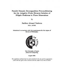
where g(x, y) := x2 − y ∂Ω . This choice of g corresponds to the fact that the analytical solution we wish to recover is the function u(x, y) = x2 − y 2 , harmonic in Ω = [0, 1] × [0, 1]. In fig.s 5.1a and 5.1b, the pointwise numerical error is shown on the whole domain, Ω, made correspondingly to PDD and quasi-PDD method, respectively, using p = 4 subdomains. The L∞ error can be read from the colorbar aside. In both pictures in Fig. 5.1, it appears clearly that the maximum error on the entire domain Ω is achieved on the interfaces, and more precisely on the interpolation nodes. This occurs according to the observation made in Section 2 concerning the maximum principle. Indeed, the error due to the Monte Carlo evaluation of the nodal values dominates over both the interpolation error and on the finite difference errors due to the local solver. This is true for both PDD and quasi-PDD methods. Moreover, ¡

¢ 2


12 0

0.01

(b)

0

0.01

0.1

0.009

0.1

0.009

0.2

0.008

0.2

0.008

0.3

0.007

0.3

0.007

0.4

0.006

0.4

0.006

0.5

0.005

0.5

0.005

0.6

0.004

0.6

0.004

0.7

0.003

0.7

0.003

0.8

0.002

0.8

0.002

0.9

0.001

0.9

0.001

1 0

0

0.2

0.4

0.6

0.8

1

y

y

(a)

1 0

0

0.2

x

0.4

0.6

0.8

1

x

Fig. 5.1. Example A. Pointwise numerical error in: (a) the PDD algorithm, and (b) the quasi-PDD algorithm. Parameters are N = 104 , ∆x = ∆y = 2 × 10−3 , λ = 102 . Table 5.1 CPU time in seconds for example A P rocessors 4 9 16

PFD 121.237 56.539 42.752

P DDT otal 106.079 35.833 20.992

P DDM onte Carlo 24.315 17.625 14.676

P DDF D 81.764 18.208 6.316

it is also clear that the quasi-PDD algorithm outperforms the PDD algorithm. The parameters used here are: N = 104 realizations, ∆x = ∆y = 2 × 10−3 grid size, λ = 102 timestepping parameter (and thus an average time-step h∆ti = 10−2 to integrate SDEs in (2.3)). In this example, concerning the Laplace equation, the hitting probability, which is the probability that a given trajectory hits the boundary between two consecutive time-steps, can be evaluated exactly, see [15]. Consequently, a relative large mean time-step could be used. Numerical experiments showed that two nodes suffice on each of the two interfaces. The local solver is based on Gauss-Seidel iteration, where the exit tolerance has been found experimentally (q = 14). In Table 5.1, the second column, labeled by PFD shows the overall computational time (in seconds) spent by the parallel finite difference algorithm for solving the problem in Example A, using p = 4, 9, and 16 processors. This corresponds to 4, 9, and 16 subdomains. In the third column the same is done, when the probabilistic domain decomposition is used. On the last two columns, the time needed in the latter algorithm is split into two parts, that concerning the Monte Carlo simulation, and that needed by the local solvers. This comparison between the two methods is made for about the same maximum error, 10−3 . It appears clearly that in both algorithms the CPU time decreases as p increases, and this behavior is more dramatic in the PDD algorithm. Also the CPU time decreases for each given number of processors passing from PFD to PDD. One can observe that the ratio between the CPU time spent in total by PDD (PDDT otal ) and that spent by PFD favorably decreases as p

13


increases, see Section 4. Example B. Consider the 2D elliptic equation with variable coefficients uxx + (6x2 + 1)uyy = 0

(5.2)

in Ω := (0, 1) × (0, 1),

subject to the boundary data (5.3)

u(x, y)|∂Ω = g(x, y), ¢ 2

where g(x, y) := x4 + x2 − y ∂Ω . Similarly to Example A, we wrote the boundary data in this way because the analytical solution of this problem is u(x, y) = x 4 +x2 −y 2 in Ω. ¡

(a)

0

0.014

(b)

0

0.014

0.1

0.1

0.012

0.012

0.2

0.2 0.01

0.3

0.5 0.006

0.6 0.7

0.004

0.008

0.5 0.006

0.6 0.7

0.004

0.8

0.8 0.002

0.9 1 0

0.4

0.008

y

y

0.4

0.01

0.3

0

0.2

0.4

0.6

0.8

1

x

0.002

0.9 1 0

0

0.2

0.4

0.6

0.8

1

x

Fig. 5.2. Example B. Pointwise numerical error in: (a) the PDD algorithm, and (b) the quasi-PDD algorithm. Parameters are N = 104 , ∆x = ∆y = 2 × 10−3 , λ = 103 .

In fig.s 5.2a, and 5.2b, the same plots as in Example A are shown, and the same comments hold. The only difference is that here three nodal points were needed in the interpolation on each interface, which choice was determined upon experimentation. Parameters are also the same used in Example A, with the only exception of the timestepping parameter λ, which has been chosen equal to 103 . Others than in Example A, here the hitting probability has to be evaluated approximately in powers of λ−1 [15]. A higher value of λ was needed here in order to ensure a good accuracy in approximating such a hitting probability. Table 5.2 shows the same comparison as in Table 5.1, and the comments are similar. The PFD method here requires more CPU time because the present problem is more elaborate, due to the variable coefficients entering the equation. Thus more iterations are needed in the linear algebraic part of the code. On the other hand, the Monte Carlo part in the PDD algorithm is faster than in Example A, because the variable diffusion implies reaching the boundary in fewer steps. Example C. Consider the elliptic equation with constant diffusion and (variable) drift terms (5.4)

∆u +

1 2 ux + uy = 0 x+1 y+1

in Ω := (0, 1) × (0, 1),


14

Table 5.2 CPU time in seconds for example B P rocessors 4 9 16

PFD 599.066 271.991 174.784

P DDT otal 317.778 75.018 30.101

P DDM onte Carlo 11.042 9.144 7.710

P DDF D 306.736 65.874 22.391

Table 5.3 CPU time in seconds for example C P rocessors 4 9 16

PFD 350.989 160.351 105.862

P DDT otal 166.728 48.374 22.585

P DDM onte Carlo 151.640 34.577 12.104

P DDF D 15.088 13.797 10.481

with the boundary data · ¸ 2 u(x, y)|∂Ω = (x + 1)2 + (y + 1)2 , 3 ∂Ω

(5.5)

the solution being given by u(x, y) = (x + 1)2 + 2(y + 1)2 /3. Figure 5.3 is analog to the previous ones, and the parameters used are the same as in Example A. In particular only two nodes on each interface have been used, but λ = 103 as in Example B. The general comments made above also apply. 0

0.02

(b)

0

0.02

0.1

0.018

0.1

0.018

0.2

0.016

0.2

0.016

0.3

0.014

0.3

0.014

0.4

0.012

0.4

0.012

0.5

0.01

0.5

0.01

0.6

0.008

0.6

0.008

0.7

0.006

0.7

0.006

0.8

0.004

0.8

0.004

0.9

0.002

0.9

0.002

1 0

0

0.2

0.4

0.6

0.8

1

y

y

(a)

1 0

0

0.2

0.4

0.6

0.8

1

x

x

Fig. 5.3. Example C. Pointwise numerical error in: (a) the PDD algorithm, and (b) the quasi-PDD algorithm. Parameters are the same as in Example B.

In Table 5.3, similar to the previous tables, one can see that now the Monte Carlo part of the PDD algorithm takes longer than in the previous examples. This fact can be attribuited to the asymmetry introduced by the drift in both directions, which ultimately requires more time steps to exit the boundary. Example D. Consider finally the Dirichlet problem for the 2D elliptic equation (5.6)

uxx + uyy − 5u = 0

in Ω := (0, 1) × (0, 1),

15

PROBABILISTIC DOMAIN DECOMPOSITION Table 5.4 CPU time in seconds for example D with two nodes per interface P rocessors 4 9 16

PFD 556.427 252.911 163.941

P DDT otal 242.453 67.190 33.496

P DDM onte Carlo 25.327 17.890 16.306

P DDF D 217.126 49.300 17.190

Table 5.5 CPU time in seconds for example D with 3 nodes per interface P rocessors 4 9 16

(5.7)

P DDT otal 242.406 72.634 36.877

P DDM onte Carlo 25.391 23.377 19.702

P DDF D 217.015 49.257 17.175

u(x, y)|∂Ω = g(x, y),

¡ ¢ where g(x, y) := e2x+y ∂Ω . The analytical solution of such a problem is u(x, y) = e2x+y , in Ω = [0, 1] × [0, 1]. In Fig. 5a and 5b, similarly to the previous cases, the pointwise numerical error is shown, made correspondingly to the PDD and the quasiPDD methods. Here only two nodes on each interface have been used. Figure 5c shows the result for three nodes on each interface (that is six nodal points in total). Note that increasing the number of nodal points yields an overall reduction of the numerical error on the whole domain. When pseudorandon numbers are used, the statistical error dominates, making it irrelevant the improvement achieved interpolating on three (instead of two) nodes on each interface. On the other hand, the time required obviously increases, see Table 5.4 and 5.5. Using quasi-random numbers, instead, which are characterized by smaller errors in computing the nodal values, an overall error reduction due to a better interpolation can be observed switching from two to three nodes. In Table 5.4 and 5.5, the same features observed in the previous examples can be seen. In Table 5.5, the CPU times related to PFD have been omitted since they coincide with those reported in Table 5.4. In fact, the comparison between PFD and PDD has been made keeping fixed the overall numerical error, which does not change passing from two to three nodes per interface, as pointed out above. Note also that the CPU times spent here in P DDM onte Carlo are about the same as those in Example A (see Table 5.1). In fact, in both examples, A and D, the numerical solution of the same system of SDEs is involved, and only a short additional time is required in Example D. This is due to the quadrature corresponding to the presence of the potential term in (5.6), see (2.2). Finally, it appears that the CPU time appreciably increases switching from two to three nodes per interface, for a higher number of processors, since this corresponds to increasing the total number of nodal points. 6. Concluding remarks. Probabilistic representations of solutions to elliptic boundary-value problems, and the ensuing possibility of using them for numerical approximations, have been known since long time. In spite of this, there is apparently in the literature only a modest body of works addressing the latter possibility, see [11, 20, 24], e.g. One reason can be certainly found in the poor performance of the Monte Carlo method. In this paper, we have first improved the overall performance of such a probabilistic numerical approach to solve linear elliptic boundary value problems. This has been done even for variable coefficient equations, including both


16

(a)

−3

x 10 3.5

0

(b)

0.1

−3

x 10

0

3.5

0.1 3

3

0.2

0.2

0.3

0.3

2.5

0.4

2.5

0.4 2

y

y

2

0.5 1.5

0.6 0.7

0.5 1.5

0.6 0.7

1

0.8

1

0.8 0.5

0.9 1 0

0.5

0.9 1 0

0

0.2

0.4

0.6

0.8

1

0

0.2

0.4

x (c)

0.6

0.8

1

x −3

x 10

0

3.5

0.1 3

0.2 0.3

2.5

0.4

y

2

0.5 1.5

0.6 0.7

1

0.8 0.5

0.9 1 0

0

0.2

0.4

0.6

0.8

1

x Fig. 5.4. Example D. Pointwise numerical error in: (a) the PDD algorithm, (b) the quasiPDD algorithm with two nodal points on each interface, evaluated by quasi-Monte Carlo, and (c) the quasi-PDD algorithm with three nodal points on each interface. Parameters are N = 10 4 , ∆x = ∆y = 2 × 10−3 , λ = 103 .

cases of variable drift and diffusion. A suitable boundary treatment, realized by means of the exponential timestepping method, was recognized as an essential ingredient and implemented. Moreover, quasi-random sequences have been successfully used, resulting in a faster convergence rate in the Monte Carlo simulations. Finally, we have adopted a “divide and conquer” strategy, represented by a domain decomposition method, where only few values are computed by Monte Carlo or quasi-Monte Carlo, thus reducing the overall inherent computational cost. Such values were used as nodes for interpolating the sought solution, then providing continuous approximations for the interfacial values, to be exploited subsequently to split the problem into several subproblems. We were then able to exploit as many processors, p, as subdomains.


17

Speed-up and scalability with p is shown, both theoretically and in a few practical examples. In closing, notice that, even a relatively coarse solution obtained by the PDD algorithm (through a Monte Carlo or quasi-Monte Carlo strategy with a moderate value of N ) could be used as the initial guess for the FD solver on the whole domain. Indeed, the exit criterion in the linear algebraic solver depends both, on the spectral radius of the iteration matrix (and thus on its spectral condition number), and on the initial guess of solution. While the former can be reduced preconditioning, which is essential in certain iterative methods, such as the iterative substructuring (deterministic domain decomposition) methods, the PDD algorithm might provide a good initial guess. Acknowledgements. We are indebted to P. Dai Prà, L. Pavarino, A. Quarteroni, M. Vianello, and O. Widlund for several useful and enlightening discussions. REFERENCES [1] Arnold, L., Stochastic Differential Equations: Theory and Applications, Wiley, New York, 1974. [2] Baldi, P., Exact asymptotics for the probability of exit from a domain and applications to simulation, Ann. Prob., 23 (1995), pp. 1644–1670. [3] Brenner, S.C., Lower bounds of two-level additive Schwarz preconditioners with small overlap, SIAM J. Numer. Anal., 21 (2000), pp. 1657–1669. [4] Buchmann, F.M., and W. Petersen, Solving Dirichlet problems numerically using the FeynmanKac representation, ETH Research Report No. 2002-01, February 2001, submitted. [5] Caflisch, R. E., Monte Carlo and quasi-Monte Carlo methods, Acta Numerica (1998), 1-49 [Cambridge University Press, Cambridge, 1998]. [6] Caflisch, R.E., Morokoff, W., and Owen, A.B., Valuation of mortgage-backed securities using Brownian bridges to reduce effective dimension, J. Comput. Finance, 1 (1997), pp. 27–46. [7] Chan, Tony F., and Mathew, Tarek P., Domain decomposition algorithms, Acta Numerica (1994), 61-143 [Cambridge University Press, Cambridge, 1994]. [8] Dryja, M., and Widlund, O.B., Domain decomposition algorithms with small overlap, SIAM J. Sci. Comput., 15 (1994), pp. 604–620. [9] Dryja, M., Smith, B.F., and Widlund, O.B., Schwarz analysis of iterative substructuring algorithms for elliptic problems in three dimensions, SIAM J. Numer. Anal., 31 (1994), pp. 1662–1694. [10] Freidlin, M., Functional Integration and Partial Differential Equations, Annals of Mathematics Studies no. 109, Princeton Univ. Press, Princeton, 1985. [11] Hausenblas, E., A Monte-Carlo method with inherent parallelism for numerical solving partial differential equations with boundary conditions, Lect. Notes Comput. Sci., 1557 (1999), pp. 117–126. [12] Higham, D.J., An algorithmic introduction to numerical simulation of stochastic differential equations, SIAM Rev., 43, No.3 (2001), pp. 525–546. [13] Hofmann, N., and Math´ e, P., On quasi-Monte Carlo simulation of stochastic differential equations, Math. Comp., 66 (1997), pp. 573–589. [14] Jansons, K.M., and Lythe, G.D., Efficient numerical solution of stochastic differential equations using exponential timestepping, J. Statist. Phys., 100, Nos.5/6 (2000), pp. 1097–1109. [15] Jansons, K.M., and Lythe, G.D. Exponential timestepping with boundary test for stochastic differential equations, SIAM J. Sci. Comput., 24 (2003) pp. 1809–1822. [16] Kalos, M.H., and Withlock, P.A., Monte Carlo Methods, Vol. I: Basics, Wiley, New York (1986). [17] Karatzas, I., and Shreve, S.E., Brownian Motion and Stochastic Calculus, 2nd ed., Springer, Berlin, 1991. [18] Kloeden, P.E., and Platen, E., Numerical Solution of Stochastic Differential Equations, Springer, Berlin, 1992. [19] L´ ecot, C., A quasi-Monte Carlo method for the Boltzmann equation, Math. Comp., 56 (1991), pp. 621–644. [20] L´ ecot, C., and El Khettabi, F., Quasi-Monte Carlo simulation of diffusion, J. of Complexity, 15 (1999), pp. 342–359.

18


[21] Mannella, R., Absorbing boundaries and optimal stopping in a stochastic differential equation, Phys. Lett. A, 254 (1999), pp. 257–262. [22] Mascagni, M., A tale of two architectures: parallel Wiener integral methods for elliptic boundary value problems, Astfalk, Greg (ed.), Applications on advanced architecture computers. Philadelphia, PA: SIAM Software-Enviroments-Tools, pp. 27–33 (1996); SIAM News, 23, No.4 (1990), pp. 8–12. [23] Morokoff, W.J., Generating quasi-random paths for stochastic processes, SIAM Rev., 40 (1998), pp. 765–788. [24] Morokoff, W.J., and Caflisch, R.E., A quasi-Monte Carlo approach to particle simulation of the heat equation, SIAM J. Numer. Anal., 30 (1993), pp. 1558–1573. [25] Morokoff, W.J., and Caflisch, R.E., Quasi-random sequences and their discrepancies, SIAM J. Sci. Statist. Comput., 15 (1994), pp. 1251–1279. [26] Morokoff, W.J., and Caflisch, R.E., Quasi-Monte Carlo integration, J. Comput. Phys., 122 (1995), pp. 218–230. [27] Moskowitz, B., and Caflisch, R.E., Smoothness and dimension reduction in quasi-Monte Carlo methods, J. Math. Comput. Modeling, 23 (1996), pp. 37–54. [28] Niederreiter, H., Random Number Generation and Quasi-Monte Carlo Methods, SIAM, Philadelphia, PA, 1992. [29] Peirano, E., and Talay, D., Domain decomposition by stochastic methods, Proceedings Fourteenth International Conference on Domain Decomposition Methods, edited by I. Herrera, D. Keyes, O. Widlund and R. Yates. Published by the National Autonomous University of Mexico (UNAM), Mexico City, Mexico, First Edition, June 2003, pp. 131–147. [30] Platen, E., An introduction to numerical methods for stochastic differential equations, Acta Numerica (1999), 197-246 [Cambridge University Press, Cambridge, 1999] [31] Press, W.H., Teukolsky, S.A., Vetterling, W.T., and Flannery, B.P., Numerical Recipes, Cambridge University Press, Cambridge, 1996. [32] Quarteroni, A., and Valli, A., Theory and application of Steklov–Poincar´ e operators for boundary-value problems, in: ‘Applied and Industrial Mathematics. Venice-1, 1989’, R. Spigler, Ed., Vol. 56, Kluwer, Dordrecht, 1991, pp. 179–203. [33] Quarteroni, A., and Valli, A., Domain Decomposition Methods for Partial Differential Equations, Oxford Science Publications, Clarendon Press, Oxford, 1999. [34] Rivlin, T.J., An Introduction to the Approximation of Functions, Dover, New York, 1981. [35] Rivlin, T.J., The Chebyshev Polynomials, Wiley, New York, 1974. [36] Spigler, R., A probabilistic approach to the solution of PDE problems via domain decomposition methods, “ICIAM 1991” (The Second International Conference on Industrial and Applied Mathematics), Washington, DC, July 8-12, 1991, Contributed Presentation, Session CP5, p. 12, Book of Astracts. [37] Strittmatter, W., Numerical simulation of the mean first passage time, University Freiburg Report No. THEP 87/12 (unpublished). [38] Talay, D., Probabilistic Numerical Methods for Partial Differential Equations: Elements of Analysis, Lecture Notes in Math., 1627, Springer, Berlin, 1996, pp. 148–196.