O(n4) algorithm for the problem was proposed (as usual, n is the number of nodes .... A node v stops being selfcontained when Tv is linked to a root node.
Dominators in Linear Time Stephen Alstrup� Peter W. Lauridsen� Mikkel Thorup� Abstract
A linear time algorithm is presented for nding dominators in control ow graphs.
1 Introduction Finding the dominator tree for a control ow graph is one of the most fundamental problems in the area of global ow analysis and program optimization [2, 3, 4, 5, 10, 15]. The problem was rst raised in 1969 by Lowry and Medlock [15], where an O(n4) algorithm for the problem was proposed (as usual, n is the number of nodes and m the number of edges in a graph). The result has been improved several times (see e.g. [1, 2, 17, 20]), and in 1979 an O(m�(m; n)) algorithm was found by Lengauer and Tarjan [14]. Finally, at STOC'85, Dov Harel [11] announced a linear time algorithm. Assuming Harel's result, linear time algorithms have been found for many other problems (see e.g. [4, 5, 10]). However, Harel never produced the details of his algorithm and the soundness of his approach has therefore been questioned. Here we rst describe some of the concrete problems in Harel's approach, of which the most important is that the algorithm presented is not linear. Secondly, using techniques that were not known at the time of Harel's work, we present a linear time algorithm for nding the dominator tree of a control ow graph, thus giving a solid foundation for all the work based on Harel's assumption. The paper is divided as follows. In section 2 the main de nitions are given. In section 3 we outline the principal dominator algorithms and in section 4 we give a linear time dominator algorithm. Finally an appendix is included, in which we brie y discuss dominators in the simpler case of reducible control ow graphs. Furthermore the appendix contains implementation details of the algorithm in section 4.
2 De nitions
A control ow graph is a directed graph G = (V; E), with jV j = n and jE j = m, in which s 2 V is a start node, from which all nodes in V are reachable through the edges in E (see e.g. [2]). If (v; w) 2 E we say that node v is a predecessor of node w and w is a successor of v. Node v dominates w if and only if all paths from s to w pass through v. Hence, if both u and v dominates w, one of u and v dominates the other. Thus the dominance relation is the re exive and transitive closure of a unique tree T, rooted in s. The tree T is called the dominator tree of G. If v is the parent of w in the dominator tree, then v immediately dominates w, denoted as idom(w) = v. � E-mail:(stephen,waern,mthorup)@diku.dk. Department of Computer Science, University of Copenhagen.
1
3 Previous dominator algorithms In this section we rst outline Lengauer and Tarjan's algorithm, since the idea behind both our algorithm and Harel's approach is to optimize subroutines used in this algorithm. Secondly, some concrete problems in Harel's approach are described.
3.1 Lengauer and Tarjan's algorithm
Lengauers and Tarjans algorithm [14] runs in O(m�(m; n)) time. Initially a Depth First Search (DFS) [19] is performed in the graph resulting in a DFS-tree T ; in which the nodes are assigned a DFS-number. In this paper we will not distinguish between a node and its DFS-number. The nodes are thus ordered such that v < w if the DFS-number of v is smaller than the DFS-number of w. The main idea of the Tarjan-Lengauer algorithm is rst to compute the so called semidominators, sdom(v), for each node v 2 V nfsg, as an intermediate step for nding dominators. The semidominator of a node v is an ancestor of v de ned as sdom(v) = minfuja path u; w1; : : :; wk ; v exists, where wi > v for all i = 1; : : :; kg. The semidominators are found by traversing the tree T in decreasing DFS-number order while maintaining a dynamic forest, F , which is a subgraph of the DFS-tree T . The following operations should be supported on F : � LINK(v; w): Adds the edge (v; w) 2 T to F . The nodes v and w are root nodes of trees in F . � EVAL(v): Finds the minimum key value of nodes on the path from v to the root of the tree in F , to which v belongs1 . � UPDATE(v; k): Sets key(v) to be k, where the node v must be a singleton tree. We will now give a more detailed description of the Tarjan-Lengauer algorithm. The forest F initially contains all nodes as singleton trees and the computation of semidominators is done as follows: � Initially we set key(v) = v for all nodes v 2 V . � The nodes are then visited in decreasing DFS-number order, i.e. v is visited before w if and only if v > w. When visiting a node v, we call UPDATE(v; k), where k = minfEVAL(w)j(w; v) 2 E g. � After visiting v, a call LINK(v; w) is made for all children w of v. After running this algorithm we have key(v) = sdom(v). The correctness of the algorithm (i.e. that when a node is updated, it is with the correct sdom-value), follows from the following theorem given by Lengauer and Tarjan [14, Theorem 4]: Theorem 1 For any node v 6= s, sdom(v) = min(S1 S S2) where S1 = fwj(w; v) 2 E ^ w < vg and S2 = fsdom(u)ju > v ^ (w; v) 2 E ^ u is an ancestor of wg. 2 1 In [14] EVAL operations only include the root of the tree in case the root is the only node in the tree. We have given the de nition above to avoid confusion, as it is this de nition which will be used in our algorithm. The Tarjan-Lengauer algorithm presented here is therefore a slight modi cation of the original algorithm. More speci cly the modi cation consists of performing the LINK(v; w) operation when v is visited in stead of when w is visited.
2
To see the connection between Theorem 1 and the algorithm above consider the visit of node v in the algorithm. Since EVAL(w) = w for w < v, S1 = fEVAL(w)j(w; v) 2 E ^ w < vg. To see that S2 = fEVAL(w)j(w; v) 2 E ^ w > vg, note that if u > v, (w; v) 2 E and u is an ancestor of w in T then u and w have already been visited. Thus u is an ancestor of w in a tree in F , so EVAL(w) includes sdom(u). Tarjan and Lengauer show that having found the semidominators, the immediate dominators can be found within the same complexity. The EVAL-LINK operations in the algorithm are performed using a slightly modi ed version of Tarjan's UNION-FIND algorithm for disjoint sets [21]. Since n LINK and m EVAL operations are performed the complexity is O(m�(m; n)). Thus a linear time algorithm can be obtained if the EVAL and LINK operations can be performed in O(n + m) time.
3.2 Harel's approach
In 1985 Harel presented an extended abstract [11] claiming a linear time algorithm. The main idea is to convert the on-line EVAL-LINK algorithm to an o�-line algorithm in much the same way as Gabow and Tarjan [9] have done with the UNION-FIND algorithm for disjoint sets. In the Gabow-Tarjan algorithm the tree, T, resulting from all UNION operations is known in advance. More speci cly this means a UNION(v; w) operations is only permitted if the edge (v; w) is in T. The FIND queries are de ned as usual, whereas UNION(v; w) is de ned as the union of the sets to which v and w belongs. The analogy with the Tarjan-Lengauer algorithm is that the tree resulting from all LINK operations is the DFS-tree T , which is computed in advance. Since Harel's paper is merely an extended abstract, very few details about parts of the algorithm is given and it is therefore di�cult to determine the correctness of his approach. We are however able to point out two concrete errors in the paper. To achieve that EVAL and LINK operations can be performed in amortized constant time, the DFS-tree is partitioned into microsets [9] of size O(logn). For each of these microsets a table, mintable, is attached, which is a lookup table for answering EVAL queries inside the microset. To construct this table a set S 0 , where jS 0 j = O(log n), of possible sdom values is computed for each microset S, so that for all UPDATE(v; k) operations v 2 S ) k 2 S 0 . The S 0 -sets are presorted and sdom-values of the nodes replaced by their rank in the sorted table. This mapping combined with a table containing the microset topology forms the entries into mintable. In the proof of theorem 1 in the paper Harel claims that: \Mintable will occupy O(n) words of storage and is computable in linear time". However even if we disregard the topology of microsets the table has entries for all possible maps from �(log n) nodes into �(log n) ranks of key values in S. There are �(log n�(log n) ) such maps, so the size of the table is super polynomial and cannot be computed in linear time. Secondly, the algorithm for computing the S 0 -sets does not compute the needed values. In [11, Theorem 3] where the completeness of the computed sets is stated, the proof of the second case in the theorem is omitted. We have concrete counterexamples [13] showing that this second case is false.
4 A linear time algorithm In this section we present a complete linear time dominator algorithm. Our approach is simpler than that of Harel, since we only wish to perform constant time EVAL and LINK operations within the scope of the Tarjan-Lengauer algorithm. Furthermore we circumvent some of the problems in Harel's construction using 3
Fredman and Willard's atomic trees [7]. As a consequence we can use the o�-line UNION-FIND algorithm directly, in stead of attempting to modify it. To be more speci c, we will construct an algorithm which performs the n LINK and UPDATE operations interspersed with m EVAL operations in O(n + m) time. As an intermediate step we will rst present a simple algorithm with complexity O(n logn + m) and then extend it to handle a special kind of update. Next we present faster algorithms for cases, in which the DFS-tree T is either a path or has few leaves. Finally we combine these algorithms to obtain a linear time algorithm.
4.1 An O(n log n + m) algorithm
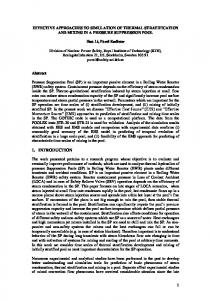
We consider a forest, F ; of trees. Recall that to each node a key is associated, which initially contains the DFS-number of the node. Let Tv denote the tree in F , to which v belongs. We will use the term selfcontained for nodes, for which EVAL(v) = key(v). Hence a node v is selfcontained if all ancestors of v in Tv have key values � key(v). Note that the de nition implies that all root nodes in F are selfcontained. A node v stops being selfcontained when Tv is linked to a root node u, for which key(u) < key(v). Lemma 1 Let nsa(v) denote the nearest selfcontained ancestor of v. (a) For any node v 2 V , we have EVAL(v) = key(nsa(v)). (b) For any node pair u; v 2 V , if nsa(v) = u at some point in the TarjanLengauer algorithm, then nsa(v) = nsa(u) in the remainder of the algorithm. Proof (a) By the de nition of selfcontained nodes key(nsa(v)) is the least key value of nodes on the path from nsa(v) to the root of Tv . By the same de nition, if nodes with key values < key(nsa(v)) were on the path from v to nsa(v) in Tv , the node with least depth among these nodes would be selfcontained. (b) By de nition nsa(u) is the rst selfcontained node on the path from u to the root of Tu . The fact that nsa(v) = u implies that Tv = Tu and that all nodes on the path from v to u in Tv have key values > key(u). By the de nition of UPDATE none of these nodes will change key values again. The node nsa(v) will therefore always be the rst selfcontained node on the path from u to the root of Tu . 2 By the second part of lemma 1 we can represent the nsa-relation e�ciently by using disjoint sets. Let each selfcontained node, u, be the canonical element of the set fvjnsa(v) = ug. By the rst part of lemma 1 an EVAL(v) operation is then reduced to nding the canonical element of the set to which v belongs, hence EVAL(v) = key(SetFind(v)). When a LINK(u; v) operation is performed, the node v will no longer be the root of Tv . Therefore a set of nodes in Tv may stop being selfcontained. Let A be this set of nodes. A node, w 2 A, is the canonical element of a set containing nodes, whose EVAL values change from key(w) to key(u) by lemma 1. We can thus maintain the structure by unifying the sets associated with nodes in A with the set associated with u. To nd the set A, a heap, supporting FindMax, ExtractMax and Union (e.g. [6, 22]), is associated with each root of a tree in F . Each heap contains the selfcontained nodes in the tree (see gure 1). The set A can then be found by repeatedly extracting the maximum element from the heap associated with v until the maximum element of this heap is � key(u). The algorithm LINK(u; v) is thus 4
1 1
2
Heap(4)
3 2
4
7
{4,5,6}
{7}
3
3
3 4
4
8
4 5
8
6
9
1
1 7
1
8
10
12
{8,9,11}
{10}
{12}
Heap(8)
12
9 10
11
Figure 1: To the left a sample DFS-tree in which the nodes are labeled by their DFS-
numbers is given. The full lines indicate the part of the tree, which has been linked, hence the node to be processed is node \3". The dotted arrows are graph edges. The numbers beside the nodes are their key values. To the right the two non-trivial heaps containing selfcontained nodes are illustrated as lists. Below the selfcontained nodes the sets associated with them are listed.
� While not Empty(Heap(v)) and key(FindMax(Heap(v))) > key(u) do � w := ExtractMax(Heap(v)); � SetUnion(u; w); /* The canonical element of the resulting set is u */ � od; � Heap(u) := HeapUnion(Heap(u); Heap(v)); Lemma 2 The algorithm presented performs the n LINK and UPDATE operations
interspersed with m EVAL operations in O(n logn) time.
Proof. At most O(n) HeapExtract, HeapFindMax and HeapUnion operations are performed. Each of these operations can be done in O(logn) time using an ordinary heap. Since the tree structure is known in advance, the set operations can be computed in linear time using the result from [9]2. It will however su�ce to use a simple disjoint set algorithm which rearranges the smallest of the two sets.2
4.2 Decreasing roots
In section 4.4 we will need the ability to decrease the key value of a node, while it is the root of a tree. We will therefore extend the algorithm from the previous section to handle the DecreaseRoot(v; k) operation, which sets key(v) = k, where v is the root of Tv . The DecreaseRoot(v; k) operation should be done in constant time. Assume that a DecreaseRoot(v; k) operation has been performed. In analogy with the LINK operation from the previous section, this may imply that some selfcontained nodes in Tv are no longer selfcontained. We should therefore remove such nodes from the heap and unify the sets associated with them, with the set associated with v, as was done in the LINK operation. However, in the algorithm from the previous section the root node v is the maximum element in the heap associated with it. In order to remove nodes from the heap we would therefore rst have to remove v, which would require O(log n) time. We should note that since If this result is used, the SetUnion operation should be changed according to the description in section 3.2. More speci cly the call would be SetUnion(parent(w); w) and the canonical element of the resulting set would be the canonical element of the set parent(w) belongs to. 2
5
the heap returns maximum values the usual decreasekey operation for heaps cannot be used. We can however take advantage of the fact that the root node will always be the maximum element in the heap it belongs to. It is therefore not necessary to explicitly insert the root into the heap before it is linked to its parent. The DecreaseRoot(v; k) operation is performed as follows. � While not Empty(Heap(v)) and key(FindMax(Heap(v))) > k do � w := ExtractMax(Heap(v)); � SetUnion(v; w); � od; � key(v) := k;
Lemma 3 We can perform d DecreaseRoot and n LINK and UPDATE operations interspersed with m EVAL operations in O(n logn + m + d) time.
Proof. We change the algorithm from the previous section by postponing the insertion of a root node, r into heap(r), until the r is linked to its parent. This has no e�ect on the complexity of EVAL and UPDATE operations stated in lemma 2. Since each node will only be in a heap once, the total number of EctractMax and SetUnion operations invoked by LINK and DecreaseRoot is still O(n). The cost of these operations can therefore be charged to the LINK operations. Since the remaining operations invoked by DecreaseRoot is done in constant time the additional complexity of the d DecreaseRoot operations is O(d).2
4.3 A linear time algorithm for paths
We consider the situation in which the tree T is a path. Recall that in the algorithms from the previous two sections we needed a heap to order selfcontained nodes. The property which distinguishes paths from trees in this context is that this ordering is induced by the path. More speci cly, any pair u; v of selfcontained nodes on the part of the path, which has been linked, are ordered such that key(v) � key(u) if and only if depth(v) � depth(u). To perform LINK operations on a path we can therefore use the algorithm from the previous section, where the heap is replaced by a stack. The algorithm for the operation LINK(u; v) on a path is thus. � While not StackEmpty and key(StackTop) > key(u) do � w := StackPop; � SetUnion(u; w);/* The canonical element of the resulting set is u */ � od; � StackPush(u); An EVAL operation on a path is performed in analogy with the previous section, hence EVAL(v) = key(SetFind(v)). Lemma 4 If the tree T is a path, we can perform the n LINK and UPDATE operations and the m EVAL operations in O(n + m) time. Proof. The stack operations are done in linear time since each node will only be on the stack once. By using the result from [9] the set operations are performed in amortized constant time. We should note that the result from [9] is more general than necessary and that it is possible to construct a simpler linear time algorithm for set operations on paths.2
6
4.4 A faster algorithm for trees with few leaves
We can take advantage of the linear time algorithm from the previous section by using it on the paths in T . More speci cly let R be the tree obtained by substituting each path in T , which consist of (at least two) nodes with at most one child, by an arti cial node. We will refer to such paths as I-paths and the arti cial nodes as I-nodes. The correspondence between R and the forest F is the following: � When the node with largest depth on an I-path is linked to its child, c, in F , the I-node is linked to c in R. � When the node with least depth on an I-path is linked to its parent, p, in F , the I-node is linked to p in R. We will use the result from section 4.2 for nodes in R and the result from the previous section tor nodes on I-paths. The above correspondence means that EVAL queries on nodes in R correspond to EVAL queries in F if, for any I-path P, key(I-node(P)) is the least key value on the part of P which has been linked. In other words we use I-node(P) to represent the minimum selfcontained node on P in R. During the processing of an I-path P the key value of I-node(P) should thus be properly updated. This is done by invoking a DecreaseRoot(I-node(P); k) operation each time a new minimum key value k is found on P. The EVAL queries on nodes on an I-path, P, will be correct, as long as the node with least depth on P has not yet been linked to its parent. We can therefore construct an interface between R and I-paths as follows. We associate a pointer, I-root, with each node on an I-path. The pointer is initially set to be NULL and when the node with least depth on an I-path is linked to its parent p, we set Iroot(v) = p, for all nodes v belonging to the I-path. The algorithm for EVAL(v) is thus (we use subscripts to distinguish between the structures EVAL operations are performed in): � if v belongs to an I-path P then � if I-root(v) =NULL then return EVALP (v) � else return minfEVALP (v);EVALR (I-root(v))g � else return EVALR (v); Lemma 5 Let l denote the number of leaves in T . We can perform m EVAL and n LINK and UPDATE operations in O(l logl + m + n) time. Proof. The I-paths are processed in linear time by lemma 4. Since the I-paths have been contracted the tree R contains O(l) nodes. Thus by lemma 3, R can be processed in time O(l log l + m + n + d), where d is the number of DecreaseRoot operations. The number of DecreaseRoot operations is however bounded by the number of nodes on I-paths.2
4.5 The linear time algorithm
From lemma 5 we have that the EVAL-LINK algorithm can be performed e�ectively on trees with few leaves. However the number of leaves is only bounded by the number of nodes. To reduce the number of leaves in T , subtrees of size � log n can be removed. We will refer to such subtrees as S-trees. Assume that all S-trees have been removed from the tree T . Then each leaf in the remaining tree must be a node in T with at least log n descendants. Thus the remaining tree has at most n= logn leaves. By lemma 5 we can therefore perform amortized constant time EVAL, LINK and UPDATE operations in the remaining tree. We now show how to process the S-trees. Recall that the LINK operations are performed in decreasing DFS-number order. This implies that EVAL operations 7
of nodes in S-trees induced by nodes outside, will only take place at a time when all links have been performed inside the structure. Furthermore the links inside Strees are performed successively, hence each S-tree can be processed independently. Analogously with I-paths we can associate a pointer S-root with each node in each S-tree, so that the EVAL operation on a node v in an S-tree becomes: EVALS (v); if S-root(v)=NULL minfEVALS (v);EVAL(S-root(v))g; otherwise To perform EVAL, LINK and UPDATE operations inside an S-tree we could use lemma 2. Alternatively we could repeat the removal of subtrees on the S-trees because of the independent nature of S-trees. Since this independence is inherited by the smaller S-trees, we can repeat this process k times to obtain the following lemma. Lemma 6 The n LINK and UPDATE operations and the m EVAL operations in the Tarjan-Lengauer algorithm can be performed in time O(mk + n log(k) n), where k 2 f1; : : :; log� ng. Proof. We repeat the removal of S-trees k times. The tree T is hereby divided into k levels. A tree at a level < k contains at most l = a= loga leaves, where a is the number of nodes in the tree. By using lemma 5 for LINK and UPDATE operations on nodes in these trees, the running time becomes O(a + l logl) = O(a). The trees at level k contains at most log(k) n nodes and for these trees we use lemma 2 for LINK and UPDATE operations. The complexity for each operation thus becomes O(log(k+1) n). Finally the EVAL operations are performed in constant time at each level, hence the complexity of an EVAL operation is O(k).2 Note that if we set k = log� n in lemma 6 the complexity is O(m log� n + n). 1
2
3
5
1
3
13
4
8
14
6
9
12
7
10
11
4
B
A
15
16
Figure 2: To the left a sample DFS-tree is given. The boxes indicate S-trees of size � 2. To the right the reduced tree is given. The nodes \A" and \B" are replacing I-paths. Note that if S-trees of size � log2 16 = 4 were removed, the tree would be reduced to a single node representing the I-path 1; 3; 8.
If k = 2 the EVAL operations are performed in constant time, but the n LINK operations requires n loglog n time by lemma 6. We will use the name microtrees for trees of size � log log n. In stead of using lemma 2 on the microtrees, we will use tabulation. As shown in section 3.2 it is not possible to tabulate trees of size �(log n) using linear time. It is however possible to tabulate microtrees of size log logn in linear time. This fact combined with the nice properties of microtrees enables us to circumvent the problems described in section 3.2. In section 4.6 we show how the microtrees are processed. 8
Theorem 2 The EVAL, LINK and UPDATE operations in the Tarjan-Lengauer algorithm can be performed in linear time.
Proof. By removing S-trees from T we get a linear time algorithm for the remaining tree by lemma 5. From each S-tree we remove microtrees and by the same lemma each S-tree can be processed in linear time. Finally to process the microtrees in linear time we use theorem 4, which is given in the next section.2 In gure 2 the division of a tree into I-paths and S-trees in one level is illustrated.
4.6 Microtree tabulation
In order to achieve the promised complexity of theorem 2 we should be able to perform constant time EVAL, UPDATE and LINK operations on forests of size � loglog n. We will do this by constructing a table containing EVAL values for all possible forest permutations. We rst show how to compute such a table assuming that a superset of sdom values is known for each microtree. Following that we show how to choose this superset. At the end of the section the promised theorem 4, which completes the dominator algorithm, is given. We start out by giving a lemma by Fredman and Willard [7].
Lemma 7 The Q-heap performs insertion, deletion, and search operations in constant time and accommodates as many as (log n)1=4 items given the availability of O(n) time and space for preprocessing and word size � log n. 2 For a set M 0 of di�erent values we de ne the rank of a value x 2 M 0 as the number of values < x in M 0. Lemma 8 If the rank of sdom-values for all nodes in a tree of size k, we can preprocess the tree in O(k) time, such that all EVAL operations can be done in constant time.
Proof. Let r denote the root of the tree. We traverse the tree in preorder and set EVAL(r)=r and for each node v 6= r set EVAL(v)=min(key(v),EVAL(parent(v))).2 Theorem 3 Assume that to each microtree M we are given a set of values M 0, where jM 0j = O(jM j) and that for all UPDATE(v; k) operations, v 2 M ) k 2 M 0. Assume also that the order in which LINK operations occur is known. It is then possible to perform constant time EVAL, LINK and UPDATE operations, given the availability of O(n) time and space for preprocessing and word size � log n.
Proof. In order to perform constant time EVAL queries we tabulate all possible forest con gurations as follows: We construct each possible tree of size � loglog n. Since in general there are at most O(2k ) trees of size k, there are at most logn such trees. For each of these trees we construct the loglog n possible ways the nodes in the tree can be partially linked. Finally for each of these forests we construct copies holding all possible permutations of ranks to nodes. In each of these forests we compute the EVAL-value for each node. We then construct a table which outputs the computed EVAL-values. By lemma 8 this computation can be done in a time proportional to the number of nodes in the trees. The number of nodes is the product of the number of trees (log n), the number of LINK's (log logn), the number of rank permutations ((C1 � log logn)log log n) and the number of nodes in each tree (log logn), thus the number of nodes is (Ci are constants): log n � loglog n � (C1 � log log n)loglog n � loglog n = log nC2 � (loglog n)2 � loglog nloglog n � 9
log nC3 � loglog nloglog n = log nC3 � lognlog loglog n = log nC3+log loglog n = O(n). To store each forest, the forest table from [9], which require loglog n space, can be used. The rank of each node require loglog logn space. If we attach a new number to each node inside the forest we can identify each node using loglog logn space. Hence each entry to the table requires loglog n+logloglog n � loglog n+loglog logn space, which will t into a computer word of size � log n. The size of the table is thus O(n) (for details see appendix 5.2.2). Given this table each microtree can be processed as follows: For each microtree we sort the sets M 0 of size O(loglog n) in linear time using lemma 7. The key value of each node is replaced by their rank in M 0 , which simply is an index into the sorted set. To carry out the operations given a microtree, we rst compute the table entry for the tree without any links. The EVAL operations are done by looking up the table and the LINK and UPDATE operations are done by updating the entry (again we refer to appendix 5.2.2 for details). Finally in order to perform UPDATE and EVAL operations we need a table which maps key values to ranks and vice versa. Since all key values are < n, this table only requires O(n) space.2 Theorem 3 requires a superset M 0 of sdom values for nodes in a microtree M. The next lemma shows how M 0 can be chosen.
Lemma 9 Let M 0 = M Sfminf(EVAL(w))j (w; v) 2 E ^ w 62 M gj v 2 M g. For all v 2 M we have that sdom(v) 2 M 0. Proof. The lemma is obviously true in case sdom(v) 2 M. Assume therefore that u = sdom(v) 62 M and that u 62 M 0 . By the de nition of semidominators a path u = w0; w1; : : :; wk?1; wk = v exists where wi > v for i = 1; : : :; k ? 1. Let wj be the last node on the path not in M. Since u 62 M 0 the node wj +1 must have a predecessor x for which EVAL(x) < u. This means that a path exists from a node u0, with u0 < u, to wj +1 on which all nodes except u0 are > v. This path can be concatenated with the path wj +1 ; : : :; wk ; v, contradicting that sdom(v) = u.2 We now complete the dominator algorithm by showing how to compute the sets M 0 of lemma 9.
Theorem 4 Let M be a microtree of size � log logn. Each EVAL, UPDATE and
LINK operation inside M in the Tarjan-Lengauer algorithm can be performed in constant time, given the availability of O(n) time and space for preprocessing and word size � logn.
Proof. By theorem 3 and lemma 9 we only need to show how to compute the sets M 0 de ned in lemma 9 in O(jM 0j) time. We will show this by induction on the visits of microtrees. Recall that the Tarjan-Lengauer algorithm visits nodes in decreasing DFS-number order. When the rst microtree is reached all nodes with larger DFS-numbers have thus been processed. By lemma 6 EVAL queries on processed nodes outside microtrees can be done in constant time. Furthermore all nodes with smaller DFS-numbers will at this stage be singleton trees. The EVAL queries required in lemma 9 can thus be performed in constant time for the rst microtree. Given an arbitrary microtree M we can therefore assume that constant time EVAL queries can be performed in microtrees containing nodes with larger DFS-numbers than the nodes in M. For nodes not in microtrees, we can compute the EVAL values needed in lemma 9 in constant time By the same arguments as above. By induction this is also the case for nodes in previously visited microtrees. 10
Finally we should note that in the proof of theorem 3, O(n) space was used for the table, which maps key values to ranks for a microtree. Since the microtrees are computed independently, this space can be re-used, so that the overall space requirement is O(n).2
5 Appendix
5.1 Algorithms for reducible graphs
The problem of nding dominators in reducible graphs has been investigated in several papers (e.g. [1, 16, 18]). The reason why reducible graphs are considered is that the control ow graphs of certain programming languages (e.g. Modula-2 [23]) are reducible. A graph is reducible if the edges can be partitioned into two disjoint sets E 0 and E 00 so that � The graph induced by the edges in E 0 is acyclic. � For all edges (v; w) 2 E 00, w dominates v. Since the edges E 00 have no in uence on the dominance relation the problem of nding dominators in reducible graphs is analogous to nding dominators in acyclic graphs. In this section we therefore assume that graphs are acyclic.
5.1.1 The former algorithm is not linear
In 1983 Ochranova [16] gave an algorithm which is claimed to have complexity O(m)3 . Unfortunately the paper does not contain a complexity analysis. In order to disprove the complexity of the algorithm it is therefore necessary to outline the behavior of the algorithm. For an acyclic graph we have the following facts: (a) If a node, x, has a single predecessor, y, then idom(x) = y. (b) If each of the successors of a node x has more than one predecessor then no node is dominated by x. Since at least one successor of the start node s will satisfy the condition in (a) the dominators can be found by starting at s and using the two facts interchangeably as follows: 1. If (a) is true for a successor, v, of the current node, w, then set idom(v) = w and the current node to v. 2. If (b) is true for all successors of the current node w then merge w and idom(w) (by unifying their successor and predecessor sets respectively). Set the current node to be the merged node. In order for the algorithm to be linear the detection of whether (a) is true in 1 should have constant time complexity. Furthermore the merge of two nodes in 2, which involves union of two sets which are not disjoint, should also have constant time complexity. The construction of such algorithms is impossible in this context. 3
Citation: "At least no counterexample was found."
11
5.1.2 A linear time algorithm
In this section we give a simple linear time algorithm for nding dominators in reducible graphs. The algorithm is constructed by combining new techniques [8] with previously presented ideas (see e.g. [1, 18]). In other words the algorithm is a compilation. The computation is divided into two main steps as follows. 1. The graph G = (V; E 0) is acyclic and can therefore be topologically sorted [12] ensuring that if (v; w) 2 E 0 then v has a lower topological number than w. 2. Now the dominator tree T can be constructed dynamically. Set s to be the root of the dominator tree T and process the nodes from V nfsg in increasing topological order as follows. (Notice that the part of T, built so far, is used for determining idom for the rest of the nodes.) � Let W = fvj(v; w) 2 E 0 g be the set of predecessors of w in G and let A be the set of ancestors in T to all nodes in W. The node idom(w) is then the node in A with the largest depth in T. Hence idom(w) can be computed by repeatedly deleting two arbitrary nodes from W and inserting the nearest common ancestor (nca) of these nodes into the set W until the set contains only one node. � After computing idom(w) the edge (w; idom(w)) is added to T. The only unspeci ed part of the algorithm is the computation of nca in a tree T which grows under the addition of leaves. In [8] an algorithm is given which processes nca and addition of leaves in constant time per operation.
Theorem 5 The algorithm above computes the dominator tree for a reducible control ow graph with n nodes and m edges in O(n + m) time.
Proof. Step 1 in the algorithm has complexity O(n + m). In step 2 each node is visited and each edge can result in a query about nca in T, so at most m nca-queries are performed, which establishes the complexity. 2
5.2 Implementation details
This section contains details about the algorithm presented in the paper. The main algorithm is described in section 5.2.1 and details about the construction and use of microtables are described in section 5.2.2.
5.2.1 The main algorithm
We assume that a DFS-search has been performed in the graph. The I-paths are removed from the tree in the following way: The child pointer of the parent to the rst node and the parent pointer of the child of the last node are removed. In stead an I-node is inserted (see gure 3). The I-node is numbered by a unique number larger than n. Furthermore the I-paths are numbered by a number > 0. The algorithm uses the following arrays in which the DFS-number of nodes are used as indices (the arrays marked � are also used in the Tarjan-Lengauer algorithm): � pred(v)� : The set of nodes w such that (w; v) 2 E. � parent(v)� : The parent of v in the DFS-tree. To simplify the EVAL operation we set parent(v) = 0 if v = 0. 12
1
1
7
7 n+k
8
8
9
9
Figure 3: An I-path and the representation of the I-path in the tree. Both child and parent pointers are illustrated
� child(v); sibling(v): Pointer to the rst child and rst sibling of v respectively in the DFS-tree.
� I-path(v): If v does not belong to an I-path, I-path(v) = 0. Otherwise Ipath(v) contains the number of the I-path to which v belongs.
� S-tree(v): True if v belongs to an S-tree. � microtree(v): True if v belongs to a microtree. � root(v): This eld is de ned for nodes in S-trees, microtrees and I-paths.
Before the root of the structure has been linked to its parent, p, root(v) = 0. Afterwards root(v) contains the number of p. � first(v): If v belongs to an I-path, this eld contains the number of the rst node on the I-path. � stack(v): If v is the rst node on an I-path, this eld contains the stack used for the I-path. � microroot(v): If v belongs to a microtree then microroot(v) is the number of the root of the microtree. � key(v)� 4: After the semidominator of v has been computed key(v) is the number of the semidominator of v. Initially key(v) = v. � bucket(v)� : The set of nodes whose semidominator is v. � dom(v)� : A number which will eventually be the number of the immediate dominator of v. The main algorithm is a slight modi cation of the Tarjan-Lengauer algorithm:
Begin constructmicrotable; /* This procedure computes the microtable */ for v := 1 to n do bucket(v) := ;; v := n; While v > 1 do begin if microtree(v) then begin microdominator(v;microroot(v)); /* see below */ v := microroot(v) ? 1; end else begin For each w 2 pred(v) do begin k :=EVAL(w); if k < key(v) then UPDATE(v; k); end; 4
In the Tarjan-Lengauer algorithm this array is called semi.
13
/* The remainder of the algorithm computes dominators */ /* from semidominators and is analogous to [14] */ For each child w of v do LINK(Sv;w); bucket(key(v)) := bucket(key(v)) fvg; While bucket(parent(v)) 6= ; do begin bucket(parent(v)) := bucket(parent(v))nfwg; k :=EVAL(w) if k < key(w) then dom(w) := k else dom(w) := parent(v);
end; v := v ? 1; end; /* While /* end; /* While /* for v := 2 to n do if dom(v) =6 key(v) then dom(v) := dom(dom(v)); else dom(v) := key(v); End; Procedure microdominator(v; root : integer);
The microdominator procedure is analogous to the main algorithm. The only real difference is that EVAL, LINK and UPDATE operations are replaced by microEVAL, microLINK and microUPDATE operations. Furthermore there are no I-paths in a microtree.
For the EVAL and LINK operations we need the following additional elds: � heap(v): A heap associated with v. � I-node(v): If v is the root of an I-path then I-node(v) is the number of the node which represents the I-path. Function EVAL(v: integer):integer; begin if v = 0 then EVAL:=1 else if microtree(v) then EVAL:=min(EVAL(root(v);microEVAL(v))) else if I -path(v) or S -tree(v) then EVAL:=min(EVAL(root(v)); key(SetFind(v))) else EVAL:=key(SetFind(v)); end; Procedure LINK(v;w: integer); begin if microtree(w) then /* w is the root of a microtree */ For each u in the microtree to which w belongs do root(u) := v else if S -tree(w) and not S -tree(v) then /* w is the root of an S-tree */ For each u in the S-tree to which w belongs do root(u) := v else if I -path(v) > 0 then begin if first(v) = v then Init-I -path(v;w) /*see below */ else if I -path(w) = I -path(v) then begin S := stack(first(v)); While not StackEmpty(S ) and key(StackTop(S )) > key(v) do begin u := StackPop(S ); SetUnion(v; u); end; if key(I -node(v)) > key(v) then DecreaseRoot(I -node(v);key(v)); StackPush(v; S ); end; end else if I -path(w) > 0 then begin /* the path is fully linked */ For each u on the I-path do root(u) := v5; /* Add I -node(w) to heap(I -node(w)) */ LINK(v;I -node(w)); 5 The I -node has not been a member of the heap while the I-path has been processed. The pseudo code for this operation is omitted to improve program clarity, as it involves creating a dummy heap and performing a HeapUnion operation on the dummy heap and heap(I -node(w)).
14
end else begin /* Neither v or w is on an I-path */ While not Empty(heap(w)) and key(HeapFindMax(heap(w))) > key(v) do begin u := HeapExtractMax(heap(w)); SetUnion(v; u); end; HeapUnion(heap(v); heap(w)); end; end; Procedure Init-I-path(v;w: integer); /* v is the rst node on an I-path and should be linked to its child w */ begin CreateStack(S ); stack(v) := S ; StackPush(v; S ); While not Empty(heap(w)) and key(HeapFindMax(heap(w))) > key(v) do begin w := HeapExtractMax(heap(w)); SetUnion(I -node(v);w); end; heap(I -node(v)) := heap(w); key(I -node(v)) := key(v); end; Procedure DecreaseRoot(v; k: integer); begin While not Empty(heap(v)) and key(HeapFindMax(heap(v))) > k do begin w := HeapExtractMax(heap(v)); SetUnion(v; w); end; key(v) := k; end; Procedure UPDATE(v; k: integer); begin key(v) := k; end;
5.2.2 The microalgorithm
In the proof of theorem 4 the forest table from [9] was suggested to store the forests. The forest from [9] support any ordering of the LINK operations, whereas in the dominator algorithm the links are performed in decreasing DFS-number order. We can therefore simplify the representation by using the DFS-traversal to represent each tree. More speci cally we start at the root and use a bitmap in which '1' means that an edge is followed down in the tree and a '0' means that we move to the parent of the current node. The tree traversal is nished when a '0' is encountered while the root is the current node. As a special case this means that a single node tree is represented by the bitmap "0". The mapping is illustrated in gure 4. In stead of representing the LINK's explicitly we can save the number of nodes in the tree, which at some point in time has been processed by the algorithm. Since the size of the forests can di�er we also need to save the size of each tree. Finally the key and EVAL values of the nodes can be saved in order of the DFS-traversal. The bitmap of an entry can thus have the following con guration [SIZEkTREEkKEYSkEVALkLINK], where SIZE and and LINK are blocks of log loglog n bits, EVAL and KEYS uses SIZE bits and TREE uses (2*SIZE-1) bits. To construct the entry of a microtree we traverse it in DFS-order and set the bits of TREE and SIZE accordingly. The KEYS are initialized to the rank of the DFS-numbers and LINK is initalized to 0. A microLINK operation is performed by incrementing the LINK value and the microUPDATE(v; k) operation is done by replacing the value of v in the entry with k. 15
1
2
3
6
4
5
Figure 4: A sample tree labeled by DFS-numbers. The bitmap of the tree is '11011000100'. The pseudo code of the microalgorithm is rather tedious and therefore omitted.
References [1] A.V. Aho, J.E. Hopcroft, and J.D. Ullman. On nding lowest common ancestors in trees. In Annual ACM Symposium on the theory of computing (STOC), volume 5, pages 115{132, 1973. [2] A.V. Aho and J.D. Ullman. The Theory of Parsing, Translation and Compiling, volume II. Prentice-Hall, Englewood Cli�s, N.J., 1972. [3] A.V. Aho and J.D. Ullman. Principles of compiler design. Addison-Wesley, Reading, MA, 1979. [4] G. Bilardi and K. Pingali. A framwork for generalized control dependence. In ACM SIGPLAN Conference on Programming Language Design and Implementation (PLDI), pages 291{300, 1996. [5] R. Cytron, J. Ferrante, B.K. Rosen, M.N. Wegman, and F.K. Zadek. E�ciently computing static single assignment form and the control dependence graph. ACM Trans. Programming Language Systems (TOPLAS), 13(4):451{490, 1991. [6] J.R. Driscoll, H.N. Gabow, R. Shrairman, and R.E. Tarjan. Relaxed heaps: An alternative to bonacci heaps with application to parallel computation. Communcation of the ACM (C.ACM), 31(11):1343{1354, 1988. [7] M.L. Fredman and D.E. Willard. Trans-dichotomous algorithms for minimum spanning trees and shortest paths. Journal of Computer and System Sciences, 48(3):533{551, 1994. [8] H.N. Gabow. Data structure for weighted matching and nearest common ancestors with linking. In Annual ACM-SIAM Symposium on discrete algorithms (SODA), volume 1, pages 434{443, 1990. [9] H.N. Gabow and R.E. Tarjan. A linear-time algorithm for a special case of disjoint set union. Journal of Computer and System Sciences, 30:209{221, 1985. 16
[10] G.R. Gao and V.C. Sreedhar. A linear time algorithm for placing �-nodes. In ACM SIGPLAN-SIGACT Symposium on the Principles of Programming Languages (POPL), pages 62{73, 1995. [11] D. Harel. A linear time algorithm for nding dominators in ow graphs and related problems. In Annual ACM Symposium on theory of computing (STOC), volume 17, pages 185{194, 1985. [12] D.E. Knuth. The art of programming, volume 1. Addison-Wesley, 1968. [13] P.W. Lauridsen. Dominators. Master's thesis, Department of Computer Science, University of Copenhagen, 1996. [14] T. Lengauer and R.E. Tarjan. A fast algorithm for nding dominators in a
owgraph. ACM Trans. Programming Languages Systems (TOPLAS), 1:121{ 141, 1979. [15] E.S. Lowry and C.W. Medlock. Object code optimization. Communication of the ACM (C.ACM), 12(1):13{22, 1969. [16] R. Ochranova. Finding dominators. Fundamentals (or Foundations) of Computation Theory, 4:328{334, 1983. [17] P.W. Purdom and E.F. Moore. Immediate predominators in a directed graph. Communication of the ACM (C.ACM), 15(8):777{778, 1972. [18] G. Ramalingam and T. Reps. An incremental algorithm for maintaining the dominator tree of a reducible owgraph. In Annual ACM Symposium on Principles of Programming Languages (POPL), volume 21, pages 287{298, 1994. [19] R.E. Tarjan. Depth- rst search and linear graph algorithms. SIAM Journal on Computing, 1(2):146{160, 1972. [20] R.E. Tarjan. Finding dominators in directed graphs. SIAM Journal on Computing, 3(1):62{89, 1974. [21] R.E. Tarjan. A class of algorithms which require nonlinear time to maintain disjoint sets. Journal of computer and system sciences, 18(2):110{127, 1979. [22] J. Vuillemin. A data structure for manipulatingpriority queues. Communcation of the ACM (C.ACM), 21(4):309{315, 1978. [23] N. Wirth. Programming in modula-2(3rd corr.ed). Springer{verlag, Berlin, New York, 1985.
17