Don't Know in Probabilistic Systems. Harald Fecher1 ... Therefore, a third value indefinite (also called don't know) ...... E.M. Clarke, O. Grumberg, and D.A. Peled.
Don’t Know in Probabilistic Systems Harald Fecher1 , Martin Leucker2 , and Verena Wolf3 1
3
Institute of Informatics, University of Kiel, Germany 2 Institute of Informatics, TU Munich, Germany Institute of Informatics, University of Mannheim, Germany
Abstract. In this paper the abstraction-refinement paradigm based on 3-valued logics is extended to the setting of probabilistic systems. We define a notion of abstraction for Markov chains. To be able to relate the behavior of abstract and concrete systems, we equip the notion of abstraction with the concept of simulation. Furthermore, we present model checking for abstract probabilistic systems (abstract Markov chains) with respect to specifications in probabilistic temporal logics, interpreted over a 3-valued domain. More specifically, we introduce a 3-valued version of probabilistic computation-tree logic (PCTL) and give a model checking algorithm w.r.t. abstract Markov chains.
1
Introduction
Abstraction is one of the most successful techniques for fighting the state space explosion problem in model checking [4]. Abstractions hide some of the details of the verified system, thus resulting in a smaller model. In the seminal papers on abstraction-based model checking, conservative abstractions for true have been studied. In this setting, if a formula is true in the abstract model then it is also true in the concrete (precise) model of the system. However, if it is false in the abstract model then nothing can be deduced for the concrete one [3]. In the 3-valued setting, the goal is to define abstractions that are conservative for both true and false. Therefore, a third value indefinite (also called don’t know), denoted by ?, is introduced that identifies when too much information is hidden to decide whether the formula evaluates to true or false in the concrete system. Thus, indefinite indicates that the abstract system has to be refined, meaning that less information should be concealed. Kripke Modal Transition Systems (KMTS, [13]) have become a popular device to model abstractions of transition systems. In the abstraction process, states of the concrete system are grouped together in the abstract system. Transitions between sets of concrete states are then classified as must or may edges. Very roughly, may edges are a kind of over approximation while must edges are a kind of under approximation. In this paper, we study abstractions for (labeled discrete-time) Markov chains (MCs). MCs are a typical underlying model for sequential probabilistic programs or probabilistic process algebras [19]. In simple words, MCs are transition systems where the transitions are enriched with transition probabilities. To get an
abstraction in the same spirit as the one for KMTS, one could again group states of the concrete system together to obtain an abstract system. Then we have to come up with a suitable notion of over and under approximation of transitions. We suggest to label transitions by intervals of probabilities, similar as in [15, 20]. The lower bound of an interval represents an under approximation while the upper bound is used for the over approximation. This motivates to define the notion of Abstract Markov Chains (AMCs) as a kind of transition system where transitions are labeled with intervals of probabilities. To compare the behavior of a given AMC and a given MC, we introduce a simulation relation, called probabilistic simulation. We call an AMC M ′ coarser or an abstraction of AMC M if M ′ simulates M and vice versa M is called finer or a refinement of M ′ . We show that the abstractions obtained by the process mentioned above are in the simulation relation. When AMCs are used in the context of abstraction, we motivate that only certain combinations of intervals are meaningful and call such AMCs delimited. Cutting arbitrary AMCs to delimited ones, also during the model checking process, will give more precise results at (nearly) no cost, as we will describe. Our main motivation for abstraction is model checking. For probabilistic systems, Jonsson and Hansson introduced Probabilistic Computation Tree Logic (PCTL) [10] that allows formulation of statements involving the measure of certain paths. We give PCTL a 3-valued semantics over AMCs. The semantics is defined, as we show, in the right manner w.r.t. abstractions: If a formula evaluates to true or false in the abstract system, it does so in the concrete system. If the result is indefinite, nothing can be said about the concrete system. We then present (two versions of) a model checking algorithm for AMCs and 3-valued PCTL. The gist of our algorithms is to use 3-valued combinations instead of boolean (as in the 2-valued case) for state formulas and to compute measures for each path property similar as in the setting of Markov decision processes [1, 7]. Recently, 3-valued-based model checking and refinement has gained a lot of interest. A framework for 3-valued abstraction is introduced in [13, 8]. In [17, 16, 2], model checking of 3-valued (or multi-valued) versions of CTL or CTL∗ have been studied. Game-based approaches allow an elegant treatment of refinement and have been presented in [18, 9] in the setting of CTL and respectively the µ-calculus. General issues for abstractions of probabilistic systems are discussed in [12, 14] while we concentrate on a specific abstraction together with dedicated model checking algorithms. The closest works to ours are [6] and [11]. In [6], Markov decision processes are proposed for abstracting of MCs. However, they only consider reachability properties while we study PCTL model checking. More importantly, our notion of simulation is coarser—thus allowing for coarser and therefore smaller abstractions—while maintaining soundness w.r.t. 3-valued PCTL. In [11]1 , criterias have been engineered that guarantee an abstraction to be optimal (in some sense). While, of course, such an optimal abstraction sounds preferable, 1
We thank the author for providing us the as yet unpublished manuscript.
the approach loses some of its elegance since—in simple words—it requires storage of much information. Furthermore, it is not clear (to us) how to obtain this information without constructing the underlying MC. We conclude our paper by discussing the pros and cons of the different approaches in detail and order them w.r.t. their precision (in a sense made precise below). Outline AMCs are derived in the next section. Before, introducing 3-valued PCTL in Section 4, we discuss the relation of measures of paths in finer and coarser systems first for reachability properties, in Section 3. The model checking algorithms for PCTL is given in Section 5. We compare our framework with existing ones in Section 6.
2
Abstract Markov Chains
To introduce our notion of abstraction, let us consider the Markov chain shown in Figure 1(a). A Markov chain consists of states labeled with propositions. The states are connected by transitions that are labeled with probabilities for taking the corresponding transitions. Following the idea of Kripke Modal Transition Systems, states of the concrete system are grouped together in the abstract system. For example, s5 and s6 form the abstract state A2 (Figure 1(b)). While in the case of transition systems, we obtain so-called may- and must -transitions denoting that there may be a transition from one state to the other, or, there is a transition for sure, we deal with lower and upper bounds on the transition probabilities here. For example, we say that we move from A2 to A1 with some probability in [0, 41 ] since we either cannot move to A1 (when in s6 ) or move to A1 with probability 41 (when in s5 ). This motivates the definition of an abstract Markov chain. Let us first fix some notation: Let AP be a nonempty finite set of propositions and B3 = {⊥, ?, ⊤} the ′ three valued truth domain. Let X be P a finite P set. For Y,′ Y ⊆ X and a function ′ Q : X × X → R let Q(Y, Y ) = y∈Y y ′ ∈Y ′ Q(y, y ). We omit brackets if Y or Y ′ is a singleton. The function Q(x, ·) is given by x′ 7→ Q(x, x′ ) for all x′ ∈ X. Furthermore let psdistr(X) = {f : X → [0, 1]} be the P set of all pseudo distribution functions on X and distr(X) = {f ∈ psdistr(X) | x∈X f (x) = 1} the set of distributions on X. Definition 1. An abstract Markov chain (AMC) is a tuple (S, P l , P u , L) where: – S is a finite set of states, – P l , P u : S×S → [0, 1] are matrices describing the lower and upper bounds for the transition probabilities between states such that for all s, s′ ∈ S, P l (s, ·) and P u (s, ·) are pseudo distribution functions and P l (s, s′ ) ≤ P u (s, s′ ) and P l (s, S) ≤ 1 ≤ P u (s, S),
(1)
– L : S × AP → B3 is a labeling function that assigns a truth value to each pair of state and proposition.
1 3
1 2
s1
1 4
s2
1 3
s3
1 3
s4
[ 14 , 32 ]
A1
A1 1 4
2 3
3 4
1 3
1 2
1
1 3
[ 13 , 43 ]
1 3
s5
3 4
s6
A2
1
[ 23 , 1]
[0, 14 ] s7
1 3
s8
A2
[0, 1]
A3
A3 [0, 34 ]
(a) Markov Chain
[0, 13 ]
(b) AMC
Fig. 1. A Markov chain and its abstraction
Note that with condition (1) we do not consider states without any outgoing transition. We call an AMC M = (S, P l , P u , L) a Markov chain (MC) if P l = P u =: P . Note that in this case P (s, ·) ∈ distr(S), for all s ∈ S. Let X be a finite set. Let g l , g u be a pair of functions in psdistr(X) with g l (x) ≤ g u (x) for all x ∈ X. We write g(x) for the interval [g l (x), g u (x)] ⊆ [0, 1] and distr (g) for the set {f ∈ distr(X) | ∀x ∈ X : f (x) ∈ g(x)}. If g l = Ql (x, ·) and g u = Qu (x, ·) for some Ql , Qu ∈ psdistr(X × X) we put distr (Q(x, ·)) = distr (g). Let us now formalize the notion of abstraction: Definition 2. Let M = (S, P l , P u , L) be an AMC and A = {A1 , A2 , .S . . , An } ⊆ 2S a partition of S, i.e. Ai 6= ∅, Ai ∩Aj = ∅ for i 6= j, 1 ≤ i, j ≤ n and ni=1 Ai = S. Then the abstraction of M induced by A is the AMC abstract(M, A) = ˜ P˜ l , P˜ u , L) ˜ given by (S, – – –
S˜ = A, P˜ l (Ai , Aj ) = mins∈Ai P l (s, Aj ) and P˜ u (Ai , Aj ) = maxs∈Ai P u (s, Aj ). For a ∈ AP the labeling of an abstract state (also called macro state) A ∈ A is given by ⊤, if L(s, a) = ⊤ for all s ∈ A, ˜ L(A, a) = ⊥, if L(s, a) = ⊥ for all s ∈ A, ?, otherwise.
Example 1. Figure 1 (a) illustrates a MC with 8 states. These states are grouped together, denoted by the dashed grey circles, to form the abstract system with three states.2 The intervals of probabilities are obtained as described before. For 2
Note that the question of how to partition the state space usually depends on where MCs are used and is beyond the scope of this paper.
(a) [ 12 , 43 ]
(b) [ 12 , 43 ]
u
s
(c) u
s [ 14 , 43 ]
v
[ 14 , 43 ]
u
[ 14 , 43 ]
v
s [ 14 , 21 ]
v
Fig. 2. Sharpening and widening the intervals
simplicity we consider a single proposition a ∈ AP that holds exactly in all grey ˜ 1 , a) =?, L(A ˜ 2 , a) = ⊥ shaded states. Thus, in the abstract system, we get L(A ˜ 3 , a) = ⊤. and L(A Scheduler In the setting of AMCs, in every state s, there is a choice for the distribution yielding the probabilities to reach successor states. This non-determinism can be resolved by means of a scheduler: A (history-dependent) scheduler for a state s0 is a function η : s0 S ∗ → distr(S × S) that maps each sequence of states s0 . . . s to a distribution in distr (P (s, ·)). The set of all schedulers for an AMC M starting in state s0 is denoted by S(M, s0 ). We write S(s0 ) if M is clear from the context. Delimited AMCs Since a scheduler is defined to select only distributions (rather than pseudo distributions), we can sharpen the definition of AMCs, motivated as follows (see also [20]): Consider the AMC M in Figure 2, (a)3 . Assume that one chooses the value 43 , i.e. P u (s, v) = P l (s, v) = 43 , from the interval [ 14 , 34 ] labeling the transition from state s to v. But then, the transition probability from state s to u is P (s, u) = 1−P (s, v) = 14 6∈ [ 21 , 43 ]. This problem does not occur in case (b) and (c) of Figure 2. The AMC in case (b) is ”finer” than (a) since [ 14 , 21 ] ⊂ [ 41 , 34 ], whereas case (c) is more abstract than (a). In the following we will “cut” AMCs so that cases with “non-constructive” information do not occur and give a transformation that refines an AMC such that the conditions are fulfilled. Thus, for the example, we change from case (a) to the finer model of (b) rather than to (c). Definition 3. For a finite set X let g l , g u ∈ psdistr(X) with g l (x) ≤ g u (x) for all x ∈ X. The cut of g l and g u is the pair cut (g l , g u ) = (f l , f u ) given by f l (x) = min{h(x) | h ∈ distr (g)}
f u (x) = max{h(x) | h ∈ distr (g)}
We call an AMC M = (S, P l , P u , L) delimited iff for all s ∈ S it holds that cut(P l (s, ·), P u (s, ·)) = (P l (s, ·), P u (s, ·)). 3
We sometimes omit outgoing transitions in examples from now on.
Summing up, cut deletes values that cannot be completed to a distribution, so no scheduler of an AMC gets lost: Lemma 1. Let M = (S, P l , P u , L) be an AMC and M ′ = (S, cut(P l , P u ), L) the delimited version of M . Then for all s ∈ S, S(M, s) = S(M ′ , s) Note that the cut operator is easy to calculate, e.g., thePlower bound of the transition probability for s to s′ will be max{P l (s, s′ ), 1 − s′′ 6=s′ P u (s, s′′ )} in the delimited version. If a lower bound is adapted no upper bound has to be adapted and vice versa. If we construct abstract(M, A) we always receive a delimited AMC if M is a MC. This is not necessarily the case if M is an AMC, even if M is delimited, as Figure 3 shows. Remark 1. In the following we assume that w.l.o.g. all considered AMCs are delimited unless otherwise stated. Extreme Distributions As will become apparent in the following, distributions taking up values on the borders of intervals, called extreme distributions, are of special interest. Let g l , g u ∈ psdistr(X) with g l (x) ≤ g u (x) for all x ∈ X and cut(g l , g u ) = (g l , g u ). For X ′ ⊆ X let ex min (g l , g u , X ′ ) be the set of distributions h ∈ distr (g) such that X ′ = ∅ implies h = g l = g u and X ′ 6= ∅ implies ∃x ∈ X ′ .h(x) = g l (x) ∧ h ∈ ex min (cut(g l , g u [x 7→ g l (x)]), X ′ \ {x}), where f [s 7→ n] denotes the function that agrees everywhere with f except at s where it is equal to n. Dually, let ex max (g l , g u , X ′ ) be the set of distributions h ∈ distr (g) such that X ′ = ∅ implies h = g l = g u and X ′ 6= ∅ implies ∃x ∈ X ′ .h(x) = g u (x) ∧ h ∈ ex max (cut (g l [x 7→ g u (x)], g u ), X ′ \ {x}). Definition 4. We say that a distribution h ∈ distr (g) min-extreme if h ∈ ex min (g l , g u , X) and max-extreme if h ∈ ex max (g l , g u , X). h is called extreme if it is min-extreme or max-extreme. (a)
(b)
(c)
u [ 12 , 34 ] s
[ 21 , 34 ] [ 14 , 21 ] v1
u
[ 14 , 21 ]
v1 v2
s [ 41 , 34 ]
[0, 14 ]
u
s
[ 12 , 43 ]
v1 v2
v2
Fig. 3. Cutting abstraction: (a) abstracted to (b) delimited to (c)
Simulation To compare the behavior described by two AMCs, we introduce the notion of probabilistic simulation that is an extension of probabilistic simulation for MCs [15]. Definition 5. Let M = (S, P l , P u , L) be an AMC. We call R ⊆ S × S a probabilistic simulation iff sRs′ implies: 1. ∀a ∈ AP : (L(s′ , a) 6=?) =⇒ L(s′ , a) = L(s, a), 2. for each h ∈ distr (P (s, ·)) there exists h′ ∈ distr (P (s′ , ·)) and δ ∈ distr(S × S) such that for all u, v ∈ S (i) δ(u, v) > 0 =⇒ uRv,
(ii) δ(u, S) = h(u),
(iii) δ(S, v) = h′ (v).
We write s ¹ s′ iff there exists a probabilistic simulation R with sRs′ . For AMC Mi = (Si , P l i , P u i , Li ), si ∈ Si , i = 1, 2 we write s1 ¹ s2 iff there exists a probabilistic simulation R on S1 ∪ S2 with s1 Rs2 in the composed AMC of M1 and M2 (which is constructed in the obvious way, assuming S1 ∩ S2 = ∅). Note that if s ¹ s′ then all possible distributions h of s are matched by a distribution h′ of s′ . The opposite does not hold, i.e., the set distr (P (s′ , ·)) may contain distributions that can not be simulated by a distribution of s. The previously defined abstraction operator induces a simulation: Theorem 1. Let M = (S, P l , P u , L) be an AMC and abstract(M, A) an abstraction of M induced by a partition A of S. Then s is simulated by its macro state, i.e. for all s ∈ S, A ∈ A s ∈ A =⇒ s ¹ A.
Example 2. Consider the MC M of Example 1, Figure 1. We have s4 ¹ A1 , for instance: Let R = {(si , A1 ) | 1 ≤ i ≤ 4} ∪ {(s5 , A2 ), (s6 , A2 )} ∪ {(s7 , A3 ), (s8 , A3 )}. ˜ A1 ) = ? condition (1) of Definition 5 is trivially fulfilled. Checking Since L(a, condition (2) for (s4 , A1 ) yields: δ(s3 , A1 ) = δ(s4 , A1 ) = δ(s6 , A2 ) = 31 and 0 for all remaining pairs. Then h′ ∈ distr(A) with h′ (A1 ) = δ(s3 , A1 ) + δ(s4 , A1 ) = 32 , h′ (A2 ) = 31 , and h′ (A3 ) = 0 is an element of distr (P˜ (A1 , ·)) such that condition (2) is fulfilled.
3
Measures and Simulation
Let us define a notion of measure for AMCs and discuss how measures are related w.r.t. simulation. Here, we study reachability properties. In the next section, we extend our study to a three-valued version of Probabilistic Computation Tree Logic (PCTL). A nonempty set Ω of possible outcomes of an experiment of chance is called sample space. A set B ⊆ 2Ω is called Borel field (or σ-algebra) over Ω if it contains Ω, Ω \ E for each E ∈ B, and the union of any countable sequence
of sets from B. The subsets of Ω that are elements of B are called measurable (w.r.t. B). A Borel field B is generated by an at most countable set E, denoted by B = hEi, if B is the closure of E’s elements under complement and countable union. A probability space is a triple PS = (Ω, B, Prob) where Ω is a sample space, B is a Borel S field over Ω,P and Prob is a mapping B → [0, 1] such that Prob(Ω) = ∞ ∞ 1 and Prob( i=1 Ei ) = i=1 Prob(Ei ) for any sequence E1 , E2 , . . . of pairwise disjoint sets from B. We call Prob a probability measure. For an AMC M = (S, P l , P u , L), let Ω = S ω be the set of trajectories (also called paths) of M . Let B be the Borel field generated by {C(π) | π ∈ S ∗ }, where C(π) = {π ′ ∈ Ω | π is a prefix of π ′ } is the basic cylinder set of π. A scheduler η ∈ S(M, s0 ) induces a probability space PS η = (Ω, B, Probη ) as follows: Probη is uniquely given by Probη (Ω) = 1 and, for n ≥ 1, Probη (C(s0 s1 . . . sn )) = h1 (s1 ) . . . hn (sn ), where hi = η(s0 . . . si−1 ), for i ∈ {1, . . . , n}, is the probability distribution selected by η. We set Probη (C(s′0 s′1 . . . s′n )) = 0 if s′0 6= s0 . Furthermore, we put π(s) = C(s) and for n = 0, 1, 2, . . . let π[n] denote the n-th state of π. When interested in the infimum of probabilities of measurable sets w.r.t. all schedulers, it suffices to consider only extreme distributions, which take values only at boundaries of intervals. A scheduler is called extreme iff it only chooses extreme distributions. The set of all extreme schedulers for state s is denoted by ES(M, s) and ES(s) if M is known. Theorem 2. For state s in an AMC, we have for every measurable set Q of the induced probability space that inf
η∈ES(s)
Prob η (Q) = inf Prob η (Q) η∈S(s)
The previous theorem can easily be shown as follows: Take a scheduler η and show that the measure is reduced (or stays the same) when changing η to an extreme distribution. Note that while there are typically infinitely many distributions leading from one state to the other in an AMC, there are only finitely many extreme distributions. Let us compare the notion of AMCs with the one of Markov decision processes (MDPs) in the three-valued setting: A Markov decision process (MDP) is a tuple M = (S, Σ, Prob, L), where S is a finite set of states, Σ is a non-empty finite set of letters, Prob : S × Σ ⇀ distr(S) is a partial function that yields for a state s and a given letter σ a distribution function for successor states. L : S × AP → B3 is a labeling function that assigns a truth value to each pair of state and proposition. The MDP M ′ = MDP(M ) induced by an AMC M = (S, P l , P u , L) is given as M ′ = (S, Σ, Prob, L) where Σ = {σh | h ∈ distr (P (s, ·)) for some s ∈ S and h is extreme}, Prob is such that Prob(s, σh ) = h if h ∈ distr (P (s, ·)) and h is extreme and Prob(s, σh ) is undefined otherwise. Thus, MDP(M ) defines a Markov decision process with the same state space as M but with (finitely-many) extreme distributions. The notion of schedulers
carries over in the expected manner, i.e. ES(M, s) = ES(MDP(M ), s) for all states s. More importantly, the infimum of the measure of some measurable set with respect to some scheduler class obviously coincides, due to Theorem 2. For the remainder of this section, let us now concentrate on reachability properties. More specifically, for an AMC M and s one of its state, a proposition a ∈ AP , α ∈ B3 and n = 0, 1, 2, . . ., let, Reach(s, a, α, n) := {π ∈ π(s) | L(π[n], a) = α and for all k < n, L(π[k], a) 6= α} and Reach(s, a, α) =
[
Reach(s, a, α, n)
n≥0
For reachability properties, it was shown in the setting of Markov decision processes (MDPs), that the infimum with respect to all schedulers agrees with the one when only so-called simple schedulers are considered [7]. A scheduler η ∈ S(M, s) is called simple iff for all π, π ′ ∈ S ∗ , s′ ∈ S, we have η(sπs′ ) = η(sπ ′ s′ ), meaning that the choice does not depend on the history π. Thus, a similar result holds for AMCs as well. The set of simple schedulers that choose only extreme distributions is denoted by SES(M, s) for AMC or MDP M . Since there are only finitely many simple extreme schedulers, the infimum is indeed a minimum. Thus, we get Lemma 2. For state s, a ∈ AP , and α ∈ B3 it holds that inf η∈S(s) Prob η (Reach(s, a, α)) = inf η∈SES(s) Prob η (Reach(s, a, α)) = minη∈SES(s) Prob η (Reach(s, a, α)) Let us now compare the behavior of two AMCs w.r.t. abstraction, i.e., simulation. We give the intuition of the following Lemma first. Let s0 ¹ s′0 . When scheduler η ∈ S(s0 ) chooses some distribution h0 , there is, according to the definition of simulation, a corresponding h′0 ∈ distr (P (s′0 , ·)). This implies that for every state s1 reachable by h0 with positive probability, there is a set of states s′11 , . . . , s′1k reachable by h′0 with positive probability, each simulating s1 . 1 Now, for s0 s1 , we can argue in the same fashion: For η(s0 s1 ) = h1 there is a corresponding h′1i for each s′0 s′1i , and so on. . . Let us be more precise: For a scheduler η ∈ S(s0 ) we define a scheduler η ′ ∈ S(s′0 ) inductively as follows: For h = η(s0 ) define η ′ (s′0 ) = h′ , where h′ is as in the definition of the simulation relation. Similarly, let s0 . . . sn be a sequence of states such that Probη (C(s0 . . . sn )) > 0 and h = η(s0 . . . sn ). By induction, there is a set of states s′n1 , . . . s′nk each simulating sn . For each s′n′ ∈ {s′n1 , . . . s′nk }, define η ′ (s′0 . . . s′n′ ) = h′ , where h′ is as in the definition of the simulation relation. Lemma 3. For α ∈ {⊤, ⊥}, a ∈ AP it holds that s ¹ s′ implies inf Prob η (Reach(s, a, α)) ≥
η∈S(s)
inf ′
η ∈S(s′ )
′
Prob η (Reach(s′ , a, α))
The previous lemma can be shown by induction on n, where n is the position where the proposition a has value α for the first time. Induction hypothesis is that ′
Prob η (Reach(s, a, α, n)) = Prob η (Reach(s′ , a, α, n)) ′′ ≥ inf η′′ ∈S(s) Prob η (Reach(s′ , a, α, n)) where η ′ is the scheduler constructed for η as described above and η may be the one for which the infimum is taken. Note that for the supremum, the corresponding result only holds when adding the paths that reach a state for which a evaluates to ?: Lemma 4. For α ∈ {⊤, ⊥}, a ∈ AP we have that s ¹ s′ implies sup Prob η (Reach(s, a, α)) ≤
′
sup Prob η (Reach(s′ , a, α) ∪ Reach (s′ , η ′ , a, ?)) η ′ ∈S(s′ )
η∈S(s)
Thus, Lemma 2 and Lemma 3 yield that the lower bound for some reachability property in the coarser system is less or equal than in the finer system. Theorem 3. Let s, s′ be states in an AMC with s ¹ s′ and a ∈ AP , and α ∈ {⊤, ⊥}. Then min Prob η (Reach(s, a, α)) ≥
η∈S(s)
min
η ′ ∈SES(s′ )
′
Prob η (Reach(s′ , a, α))
In simple words, the previous theorem says that when the minimum of a reachability property is at least p in the coarser system, it is so in the finer system as well.
4
3-valued PCTL
Recall that AP denotes a nonempty finite set of propositions. The set of Probabilistic Computation-Tree Logic (PCTL) [10, 5] formulas over AP , denoted by PCTL, is the set of state-formulas ϕ inductively defined as follows: ϕ ::= true | a | ϕ ∧ ϕ | ¬ϕ | [Φ]⊲⊳p
Φ ::= Xϕ | ϕ U ϕ
where ⊲⊳ ∈ {≤, }, p ∈ [0, 1] and a ∈ AP . The formulas defined by Φ are called path-formulas4 . In the setting of AMCs, a state might no longer just satisfy or refuse a formula, but a third value ? (don’t know) is appropriate. Consequently, we define the satisfaction of a formula w.r.t. a state as a function into B3 , which forms a complete lattice ordering the elements as ⊥ < ? < ⊤. Joins and meets in this lattice are denoted by ⊔ and ⊓, respectively. Complementation is denoted by ¯, where ⊤ and ⊥ are complementary to each other while ? =?. 4
To simplify the presentation, we omit the bounded until operator given in [10], which could easily be added.
[s, true]] =⊤ [s, false]] = ⊥ [s, a]] = L(s, a) [s, ϕ1 ∧ ϕ2] = [s, ϕ1] ⊓ [s, ϕ2] [s, ¬ϕ1] = [s, ϕ1] 8 8 l l > < ⊤ if P r (s, Φ, ⊥) ≥ 1 − p < ⊤ if P r (s, Φ, ⊤) ≥ p l l ⊥ if P r (s, Φ, ⊤) > p [s, [Φ]≥p] = ⊥ if P r (s, Φ, ⊥) > 1 − p [s, [Φ]≤p] = > : : ? otherwise ? otherwise [π, Xϕ1] = [π[1], ϕ1] 8 < ⊤ if ∃i.([[π[i], ϕ2] = ⊤ and ∀0 ≤ j < i.[[π[j], ϕ1] = ⊤) [π, ϕ1 U ϕ2] = ⊥ if ∀i.([[π[i], ϕ2] 6= ⊥ =⇒ ∃0 ≤ j < i.[[π[j], ϕ1] = ⊥) : ? otherwise, Fig. 4. Semantics of PCTL formulas
When a formula evaluates in a state to ⊤ or ⊥, we sometimes say that the result is definite. Otherwise, we say that it is indefinite. Similarly, we say the result holds for sure or is violated for sure if it evaluates to ⊤ respectively ⊥. We say it may be true or may be false if it evaluates to ?. Given an AMC M = (S, P l , P u , L) and a PCTL formula ϕ we define the satisfaction function [s, ϕ]] for state s ∈ S and [π, Φ]] for trajectory π ∈ S ω inductively as shown in Figure 4, where P rl (s, Φ, α) = inf η∈SES(s) Prob η ({π ∈ π(s) | [π, Φ]] = α}) for α ∈ B3 . For the cases ⊲⊳ = < and ⊲⊳ = > the value of [s, [Φ]⊲⊳p] is similar to the cases ≤ and ≥, respectively, but we exchange ≤ by < and vice versa. To understand why the above semantics is sound with respect to the notion of simulation in Definition 5 we discuss each operator in the following and state the soundness result later in Theorem 4. Case true, false, a, ∧, ¬: The semantics is defined as expected for the base and boolean cases. Case X and U: The truth value of [π, Xϕ1] equals the result of ϕ1 in state π[1]. A trajectory π satisfies the formula ϕ1 U ϕ2 for sure, if ϕ1 holds for sure until ϕ2 holds for sure. It is violated, if either ϕ2 is always wrong for sure, or otherwise ϕ1 is violated before. Case [Φ]≥p : For [Φ]≥p , the situation is slightly more involved. First, we remark that Lemma 2 holds also for PCTL path properties, i.e. that is suffices to consider simple extreme schedulers instead of arbitrary ones. Lemma 5. Let M be an AMC, s one of its states, Φ a path property of PCTL, α ∈ B3 , and Q = {π ∈ π(s) | [π, Φ]] = α}. Then inf Prob η (Q) =
η∈S(s)
inf
η∈SES(s)
Prob η (Q) =
min
η∈SES(s)
Prob η (Q)
In view of the simulation relation we can show that coarser systems yield even lower bounds than finer systems. Lemma 6. For states s, s′ in an AMC with s ¹ s′ and Φ a path property of PCTL, α ∈ {⊤, ⊥}, Q = {π ∈ π(s) | [π, Φ]] = α}, Q′ = {π ∈ π(s′ ) | [π, Φ]] = α}
we have min
η∈SES(s)
Prob η (Q) ≥
min
η ′ ∈SES(s′ )
′
Prob η (Q′ )
The previous lemmas can easily be shown as their counterparts for reachability properties listed in the previous section. For [Φ]≥p , we measure the paths starting in s for which Φ evaluates to ⊤ and check whether the lower bound of this measure is greater or equal to p. If so, the result is ⊤ and for a finer state s′ with s′ ¹ s this measure is also greater than p. For scheduler ηP∈ SES(M, s′ ) we set pηα = Prob η ({π ∈ π(s′ ) | [π, Φ]] = α}) and observe that α∈B3 pηα = 1. If the measure of the paths starting in s for which Φ evaluates to ⊥ is greater than 1 − p, then this is also the case for s′ , i.e. pη⊥ > 1 − p. Therefore, this leaves less than 1 − (1 − p) = p for pη⊤ + pη? . In other words, even if pη? is added to pη⊤ , the constraint ≥ p cannot be met. Therefore, we decide for ⊥. Case [Φ]≤p : For [Φ]≤p , we consider the measure of paths starting in s for which Φ evaluates to ⊤. If the lower bound is already bigger than p, it is so especially so for s′ and we decide for [Φ]≤p as ⊥. Similarly, if for enough paths Φ evaluates to ⊥, we can be sure that the measure of paths satisfying Φ is small. If P rl (s, Φ, ⊥) ≥ 1 − p then in the finer system for all η ∈ SES(M, s′ ) we get pη⊥ ≥ 1 − p. But then pη? + pη⊤ ≤ 1 − (1 − p) = p. In other words, even if pη? is added to pη⊤ , the constraint ≤ p is fulfilled and we go for ⊤. The following theorem states that our framework developed so far can indeed be used for abstraction based model checking and follows easily from Lemma 6 and the discussion above. In simple words, it says that the result of checking a formula in the abstract system agrees with the one for the finer system, unless it was indefinite. Theorem 4. Let s and s′ be two states of an AMC M with s ¹ s′ . Then for all ϕ ∈ PCTL: [s′ , ϕ]] 6= ? implies [s, ϕ]] = [s′ , ϕ]]. Observe that the 3-valued PCTL semantics of an MC understood as an AMC coincides with the usual 2-valued PCTL semantics for Markov chains.
5
Model Checking 3-valued PCTL
In this section, we discuss two model checking algorithms for 3-valued PCTL. As for CTL, both model checking algorithms work bottom-up the parse tree of ϕ. Hence, it suffices to describe their steps inductively on the structure of ϕ. Each state s is labeled with a function ts assigning to each subformula its truth value. ts is defined directly for true, false, a, ϕ1 ∧ ϕ2 , and ¬ϕ1 according to the definition of their semantics. For [Φ]⊲⊳p , ts can easily be determined, provided the lower bound of a measure of paths for some path property (denoted by P rl in Figure 4) can be computed. Therefore, it remains to show how to compute
the lower bound of the measure of paths for which an until or next-step formula evaluates to ⊤, ⊥, and ?. Let us discuss Φ := ϕ1 U ϕ2 . The treatment of the nextstep operator is similar but easier and is omitted here. Thanks to Theorem 2, computing the measure for an until property becomes (technically) easy, since only extreme distributions have to be considered. Reduction to MDP model checking The first idea is to convert an AMC M to an MDP MDP(M ) and reuse existing methods for computing path properties on MDPs. Before translating M , we can assume that for every state, we know the truth values of ϕ1 and ϕ2 . We annotate MDP(M ) with (two-valued) propositions corresponding to the values of ϕ1 and ϕ2 in M . More specifically, label a state s of MDP(M ) by the (new) propositions aϕ1 and aϕ2 , if ϕ1 respectively ϕ2 evaluates ¯ϕ2 , if ϕ1 respectively ϕ2 are ⊥. Now, to ⊤ in s. Label s by propositions a ¯ϕ1 and a considering the semantics of the until operation as shown in Figure 4, it is easy to see that ϕ1 U ϕ2 on a path of M evaluates to ⊤ iff aϕ1 U aϕ2 on the same path (of MDP(M )) evaluates to true. Similarly, it is easy to see that ϕ1 U ϕ2 aϕ2 ) evaluates to true. on a path of M evaluates to ⊥ iff ¬(¬¯ aϕ1 U ¬¯ Using the reduction to an MDP model checking problem for until properties, we have completed the first algorithm that is mainly used to give an upper bound on the complexity of the model checking problem. Complexity Computing the semantics for an AMC M and a formula ϕ ∈ PCTL bottom-up for every state can be done in linear time, provided the measures for path properties are given. For every state s with k outgoing transitions, one can obtain, in the worst case, k! extreme distributions. Thus, the size of MDP(M ) is at most exponential in the size of M , where, as expected, the size of M , denoted by |M | is the number of states plus the number of transitions, i.e., pairs (s, s′ ) for which P l (s, s′ ) > 0. Computing the measure for a path property in an MDP M ′ is polynomial with respect to the size of M ′ (states plus non-zero transitions) [7]. Thus, overall, we get: Theorem 5. Given an AMC M = (S, P l , P u , L) and a PCTL formula ϕ, then the algorithm outlined in this section labels every state s ∈ S with ts (ψ) = [s, ψ]] for each subformula ψ of ϕ in time polynomial w.r.t. O(2|M| log |M| ) and linear w.r.t. the size of ϕ, where |M | denotes the size of M . Fixpoint computation The reduction to an MDP for computing path properties suffers from the effort spent for computing all extreme distributions. Therefore, we have implemented a version of the algorithm that is based on fixpoint iteration. This algorithm, while (only) approximating the minimal result in question, chooses (and computes) extreme distributions in an on-the-fly fashion, leading to huge space gains. Our approach is inspired by the treatment in [1, 5] done for MDPs. Let us define the sets:
W⊤+ W⊤− W⊥+ W⊥−
= {s | ts (ϕ2 ) = ⊤} = {s | ts (ϕ2 ) 6= ⊤ and ts (ϕ1 ) 6= ⊤} = {s | ts (ϕ2 ) = ⊥ and ts (ϕ1 ) = ⊥} = {s | ts (ϕ2 ) 6= ⊥}
To simplify our presentation, we say that Φ evaluates in a state to some value in B3 if it evaluates to that value on all paths starting in this state. Φ holds in W⊤+ for sure and is violated for sure in W⊤− . However, the result is ⊥ in W⊥+ since ϕ1 as well as ϕ2 is ⊥. In W⊥− the formula is not necessarily violated. Let pmin abbreviate (P rl (s, Φ, α))s∈S . We obtain pmin as least fixpoint of α α the iteration described in the following: First, let Del be the set of all pairs of delimited pseudo distribution functions on S and b ∈ {l, u}. Consider the minimization/maximization function ξ b : 2S × Del × (S → [0, 1]) → [0, 1] that is given by ξ b (∅, (g l , g u ), x) = 0 and for S ′ 6= ∅ ξ l (S ′ , (g l , g u ), x) = g l (sl ) · x(sl ) + ξ l (S ′ \ {sl }, cut(g l , g u [sl 7→ g l (sl )]), x) if x(sl ) = mins′ ∈S ′ x(s′ ), ξ u (S ′ , (g l , g u ), x) = g u (su ) · x(su ) + ξ u (S ′ \ {su }, cut(g l [su 7→ g u (su )], g u ), x) if x(su ) = maxs′ ∈S ′ x(s′ ). Note that ξ b (S, (g l , g u ), x) sorts the states s ∈ S ′ according toP their values in x and chooses h ∈ distr (g) that minimizes/ maximizes the value s∈S h(s) · x(s).5 Let S + , S − ⊆ S. We use ξ b to define the function Fb(S − ,S + ) : (S → [0, 1]) → (S → [0, 1]) that determines the next iteration step by if s ∈ S + , 1 b if s ∈ S − , F(S − ,S + ) (x)(s) = 0 b l u ξ (S, (P (s, ·), P (s, ·)), x) otherwise. Furthermore, let x0 denote the function that maps everything to 0. Theorem 6. The least fixpoint (w.r.t. point wise extension of the order of the real numbers) of the function Fb(S − ,S + ) can be used to calculate the values pmin α : l pmin ⊤ (s) = (⊔n∈IN F(W − ,W + ) ⊤
pmin ⊥ (s) 5
= 1−
⊤
(n)
(x0 ))(s)
(⊔n∈IN Fu(W + ,W − ) (n) (x0 ))(s) . ⊥ ⊥
The function ξ b is well defined, i.e., the same value is obtained if another maxiP mal/minimal state s′ is considered. This follows from the fact that min{ s∈S ′ h(s) | P h ∈ distr (g)} = min{ s∈S ′ h(s) | h ∈ distr (cut(g l , g u [s′ 7→ g l (s′ )]))} for all S ′ ⊆ S with s′ ∈ S ′ .
(a)
(c)
(b) u
4 10 3 10
s
2 10
v1
2 10
u
1 10
s
′
3 10
σ1 v1 w σ2
1 10
v2
4 10
1 10
2 10
s s′
3 10
w
4 10
v2
1 10
2 10
(d) u
u
1 4 [ 10 , 10 ] 2 [ 10 ,
v1 s s′
w
3 ] 10
2 3 [ 10 , 10 ]
v1 w
3 10 4 10
v2
1 , [ 10
4 ] 10
v2
Fig. 5. Abstraction by MDPs vs. AMCs
The proof goes along the lines of the proof for MDPs (see [1, Chapter 3] for details). Let us give an example showing that the cut in the definition of the fixpoint operator in Theorem 6 to calculate the probabilities for [Φ]⊲⊳p is indeed important: Example 3. Let us consider the AMC shown in Figure 3 (a) (page 6) and Φ = ϕ1 U ϕ2 . Assume that ts (ϕ1 ) = tv2 (ϕ1 ) = tu (ϕ2 ) = ⊤ and all remaining truth values for ϕ1 and ϕ2 are ⊥. Furthermore, assume that there is a [1, 1]transition from v2 back to itself. Then we get: W⊤+ = {u} and W⊤− = {v1 }. For example, the maximization function ξ u chooses P l (s, u) = P u (s, u) = 43 since 1 = max{1, 0, 0} = max{x(u), x(v1 ), x(v2 )} after the first iteration step and due to the cut operation P (s, v1 ) = [ 14 , 14 ] and P (s, v2 ) = [0, 0]. Hence, P ru (s, Φ, ⊤) = 43 · 1 + 41 · 0 + 0 · 0 = 43 . W⊥+ = {v1 , v2 } and W⊥− = {u}. Altogether we get P r(s, Φ, ⊤) = [ 12 , 43 ], P r(s, Φ, ⊥) = [ 41 , 21 ], P r(s, Φ, ?) = [0, 0]. Note that we get the intervals shown in Figure 3 (c). Thus, the subsequent cut in the definition of the fixpoint operator is necessary since the values in Figure 3 (b) yield less precise results.
6
Alternatives to AMCs
Let us discuss alternative approaches for abstraction of Markov chains. For reasons of space limitation, we keep the discussion informal. Generally, Markov Decision Processes (MDPs) are considered to be abstractions for Markov chains. MDPs extend the model of MCs by allowing several distribution functions in each state (see Figure 5 (c)). Thus, when merging states to obtain an abstraction, one could define the corresponding distribution functions, as indicated in Figure 5 (a)–(c). Hence, the result would be an MDP. Now, one might be tempted to use existing model checking theory for PCTL and MDPs to reason about the underlying Markov chain. However, this is not possible since, as far as we know, there is no 3-valued notion of PCTL for MDPs (not to mention, we need one that suits the role in the abstraction defined here).
When interested in reachability properties, the approach is possible and was pursued in [6]. Let us call the approach AMDP. Actually, the model checking algorithms presented in the previous section considers the AMC as an MDP with extreme distributions, but only when computing the minimal probabilities of path properties. Of course, one could have developed such a 3-valued version of PCTL for MDPs as opposed for AMCs, as done here. But actually, the 3-valued PCTL semantics given in Section 4 can easily be taken over for such a 3-valued PCTL semantics for MDPs. However, there is an intrinsic difference in the approach using AMCs and the one based on MDPs. An MDP can easily be abstracted to an AMC. For example, for the MDP shown in Figure 5 (c), we would get the AMC shown in Figure 5 (d). But using intervals, one reduces more information. This has two implications, one theoretical and one practical. Our semantics for PCTL path properties compares only extreme distributions. Probabilities that are not the bound of some transition probability interval are not considered. However, we might consider all extreme distributions. For example, one extreme 4 2 3 1 distribution for the AMC in Figure 5 (d) is (u 7→ 10 , v1 7→ 10 , w 7→ 10 , v2 7→ 10 ), 6 , where which is not present in Figure 5 (c). Now, consider ϕ = [X(au ∨ aw )]≤ 10 proposition au (aw ) is ⊤ in state u (respectively w) and ⊥ in all other states. Then the macro state in Figure 5 (c) provides ⊤ for ϕ but for the AMC in Figure 5 (d) the result is ?. Thus, our results might sometimes be less precise. From the practical side, using MDPs, one reduces the number of states but basically all distributions are kept. But storing all distributions causes no memory savings and it is questionable whether such an abstraction does indeed satisfy practical needs. In our approach, on the other hand, if, for example, a third distribution 2 2 3 3 denoted by σ3 with (u 7→ 10 , v1 7→ 10 , w 7→ 10 , v2 7→ 10 ) would be present in Figure 5 (c), we obtain the same AMC, thus, reducing the memory requirments. A different approach was taken in [11]. There, criterias have been engineered that guarantee an abstraction to be optimal (in some sense). Let us call this approach O. While, of course, such an optimal abstraction sounds preferable, it turns out that neither AMCs nor MDPs carry enough information to be optimal. In simple words, the approach loses some of its elegance since it requires to store much information. Furthermore, it is not clear (to us) how to obtain this information without constructing the underlying Markov chain. The author of [11] therefore suggests as well a more simple approximation of the optimal abstraction, which we call S. In simple words, S is similar to AMCs but does not use the cut operator to optimize the information present in AMCs. Let us discuss Example 15 of [11]: Consider Figure 6 and Φ = [X¬au1 ]>0 where au1 is true in u1 and false in all other states. For the approach S the result in u0 is ? because the sum of the two zero values of the lower bounds to the direct successors ud and u0 are added which yields 0 + 0 = 0 (see [11, Example 15]). In our setting after the first chosen zero value, say P l (u0 , ud ) = P u (u0 , ud ) = 0 through the cut the next choice is P l (u0 , u0 ) = 1 − 0.01 = 0.99. The resulting extrem distribution is (ud 7→ 0, u0 7→ 0.99, u1 7→ 0.01) which leads to [u0 , Φ]] = ⊤.
[0, 1] [0, 0.99]
ud
[1, 1]
u1
[0.5, 0.64]
[0.36, 0.5]
u0
[0, 0.01] Fig. 6.
Thus, results based on S are less precise than the results obtained with our method. In terms of memory, S and AMC are comparable, provided the fixpoint computation method is used. Note that [11] does not address the question of model checking. Summarizing, with abstraction one loses information usually by reducing space requirements. All approaches have in common, that states are grouped together to form an abstract system. They differ in the information that is kept for transitions. By means of precision, we can order the approaches S < AMC < AMDP < O, where a < b means that a is less precise than b, when for some concrete system, the same states are grouped together. In terms of memory usage, we can order the approaches as S = AMC < AMDP < O, where a < b means that a consumes less memory than b, when for some concrete system, the same states are grouped together.
7
Conclusion
In this paper, we have extended the abstraction-refinement paradigm based on three-valued logics to the setting of probabilistic systems. We have given a notion of abstraction for Markov chains. In simple words, abstract Markov chains are transition systems where the edges are labeled with intervals of probabilities. We equipped the notion with the concept of simulation to be able to relate the behavior of abstract and concrete systems. We have presented model checking for abstract probabilistic systems (i.e. abstract Markov chains) with respect to specifications in a probabilistic temporal logic, interpreted over a 3-valued domain. More specifically, we studied a 3valued version of PCTL. The model checking algorithm turns out to be quite similar to the ones developed in the setting of checking PCTL specifications of Markov decision processes. Thus, using the intuitive concept of intervals allows to refrain from saving all probability distributions present in concrete systems but storing only boundaries, while allowing to adapt existing theory of model checking probabilistic systems. Our work can be extended into several directions. First, further insight in which and how to split states is desirable, when the model checking result is indefinite. It would also be interesting to extend our setting towards the more expressive logic PCTL∗ or to the setting of continuous-time Markov chains.
References 1. Christel Baier. On the algorithmic verification of probabilistic systems. Universit¨ at Mannheim, 1998. Habilitation Thesis. 2. M. Chechik, B. Devereux, S. Easterbrook, and A. Gurfinkel. Multi-valued symbolic model-checking. ACM Transactions on Software Engineering and Methodology (TOSEM), 12:371–408, 2003. 3. E. Clarke, O. Grumberg, and D. Long. Model Checking and Abstraction. In Proc. of POPL, pages 342–354, New York, January 1992. ACM. 4. E.M. Clarke, O. Grumberg, and D.A. Peled. Model Checking. MIT press, December 1999. 5. C. Courcoubetis and M. Yannakakis. The complexity of probabilistic verification. Journal of the ACM, 42(4):857–907, July 1995. 6. P. D’Argenio, B. Jeannet, H. Jensen, and K. Larsen. Reduction and refinement strategies for probabilistic analysis. In PAPM-PROBMIV, pages 57–76, 2002. 7. Luca de Alfaro. Formal Verification of Probabilistic Systems. PhD thesis, Stanford University, 1997. Technical report STAN-CS-TR-98-1601. 8. P. Godefroid and R. Jagadeesan. On the expressiveness of 3-valued models. In Verification, Model Checking and Abstract Interpretation (VMCAI), volume 2575 of LNCS, pages 206–222, 2003. 9. O. Grumberg, M. Lange, M. Leucker, and S. Shoham. Don’t know in the µ-calculus. In Proc. VMCAI’05, volume 3385 of LNCS. Springer, 2005. 10. H. Hansson and B. Jonsson. A logic for reasoning about time and reliability. Formal Aspects of Computing, 6:512–535, 1994. 11. M. Huth. On finite-state approximants for probabilistic computation tree logic. Theoretical Computer Science. to appear. 12. M. Huth. An abstraction framework for mixed non-deterministic and probabilistic systems. In Validation of Stochastic Systems, pages 419–444, 2004. 13. M. Huth, R. Jagadeesan, and D. Schmidt. Modal transition systems: A foundation for three-valued program analysis. In European Symposium on Programming (ESOP), volume 2028, pages 155–169, 2001. 14. Michael Huth. Abstraction and probabilities for hybrid logics. In Qualitative Aspects of Programming Languages, 2004. 15. B. Jonsson and K. Larsen. Specification and refinement of probabilistic processes. In Proc. 6th IEEE Int. Symp. on Logic in Computer Science, 1991. 16. B. Konikowska and W. Penczek. Model checking for multi-valued computation tree logics. In Beyond two: theory and applications of multiple-valued logic, pages 193–210. Physica-Verlag GmbH, 2003. 17. B. Konikowska and W. Penczek. On designated values in multi-valued CTL∗ model checking. Fundamenta Informaticae, 60(1–4):221–224, 2004. 18. S. Shoham and O. Grumberg. A game-based framework for CTL counterexamplesand 3-valued abstraction-refinemnet. In Computer Aided Verification (CAV), volume 2725 of LNCS, pages 275–287, 2003. 19. R. van Glabbeek, S. Smolka, B. Steffen, and C. Tofts. Reactive, generative, and stratified models of probabilistic processes. In Logic in Computer Science, pages 130–141, 1990. 20. W. Yi. Reasoning about uncertain information compositionally. In Proc. of the 3rd International School and Symposium on Real-Time and Fault-Tolerant Systems, volume 863 of LNCS. Springer, 1994.