DOUBLE-LAYERED DYNAMICS: A UNIFIED THEORY OF PROJECTED DYNAMICAL SYSTEMS AND EVOLUTIONARY VARIATIONAL INEQUALITIES Monica-Gabriela Cojocaru1 , Patrizia Daniele2 , Anna Nagurney3 1 Department
of Mathematics & Statistics, University of Guelph, Ontario, Canada email:
[email protected]
2 Department
of Mathematics & Computer Science, University of Catania, Italy email:
[email protected]
3 Department
of Finance & Operations Management, Isenberg School of Management
University of Massachusetts, Amherst, Massachusetts 01003, USA email:
[email protected]
December 2004; revised April 2005 Abstract. In this paper we continue the study of the unified dynamics resulting from the theory of projected dynamical systems and evolutionary variational inequalities, initiated by Cojocaru, Daniele, and Nagurney. In the process we make explicit the interdependence between the two timeframes used in this new theory. The theoretical results presented here provide a natural context for studying applied problems in disciplines such as operations research, engineering, in particular, transportation science, as well as in economics and finance.
Key words: Projected dynamical systems, Evolutionary variational inequalities, System dynamics, Multiple timescales, Dynamic networks, Network equilibria, Operations research, Transportation science, Economics.
1
2
1. Introduction In [7] the authors built the basis for merging the theory of projected dynamical systems (PDS) and that of evolutionary variational inequalities (EVI), in order to further develop the theoretical analysis and computation of solutions to applied problems in which dynamics plays a central role. The two theories have developed in parallel and have been advanced by the need to formulate, analyze, and solve a spectrum of dynamic problems (oftentimes, network-based) in such disciplines as operations research, and in engineering, notably, in transportation science, as well as in economics and finance. The intriguing feature of the merger is that it allows for the modeling of problems that present two (theoretically) distinct timeframes, most simply put, a big scale time and a small scale time. The existing literature has focused on understanding human decision-making for a specific timescale rather than viewing decision-making over multiple timescales (see, e.g, [4], [13], [28], [36], and the references therein). The ability to capture multiple timescales can also further support combined strategic and operational decision-making and planning. There are new exciting questions, both theoretical and computational, arising from this “multiple time structure.” In the course of answering these questions, a new theory is taking shape from the synthesis of PDS and EVI, and, as such, it deserves a name of its own; we shall call it double-layered dynamics. This paper gives novel theoretical insights into the type of problems modeled by a double-layered dynamics. Generally, an EVI model gives a curve of equilibria of the underlying problem, over a finite time interval [0, T ]. For almost all t ∈ [0, T ], there is a PDS, which we shall call P DSt , that describes the time evolution of the underlying problem towards an equilibrium point on the curve of equilibria, corresponding to the moment t. However, this evolution time for the respective P DSt , which we shall denote by τ , is different from t. As in the case of PDS theory [23], [4], [47], [37], we can establish results about the stability of this curve of equilibria. Even more importantly, we make precise the
3
relation between t and τ since in order for the PDS/EVI models to be useful, it is essential that the t and τ are related in an intuitively clear, meaningful way. The results in this paper are based on various monotonicity properties of the underlying vector field of PDS/EVI. This is extremely valuable, since monotonicity concepts are present in both PDS and EVI theories; in PDS they are used to study stability of perturbed equilibria and in EVI they are used as essential conditions for the existence of solutions. The outline of the paper is as follows: Section 2 contains brief introductions to PDS and EVI. Section 3 overviews the rigorous formulation of the double-layered dynamics theory and discusses the question of uniqueness of such curves of equilibria in the PDS/EVI context. Section 4 shows the stability properties of such curves in a given neighborhood and establishes the relation between the two timeframes and their estimates. Section 5 presents an illustrative dynamic traffic network numerical example. We close this paper with a few concluding remarks in Section 6.
4
2. Brief overview of the foundations of PDS and EVI theories A thorough introduction to both theories and applications of PDS and EVI has been presented in our earlier paper [7]. Here we outline only the necessary theoretical facts in order to insure a self-contained presentation of this work. 2.1. PDS. In the early ’90s, Dupuis and Nagurney [18] introduced a class of dynamics given by solutions to a differential equation with a discontinuous right-hand side, namely dx(t) = ΠK (x(t), −F (x(t))). (1) dt In their formulation K is a convex polyhedral set in Rn , F : K → Rn is a Lipschitz continuous function with linear growth and ΠK : R × K → Rn is the Gateaux direcPK (x − δF (x)) − x tional derivative ΠK (x, −F (x)) = lim+ of the projection operator δ→0 δ PK : Rn → K, given by ||PK (z) − z|| = inf ||y − z|| (see [17] and [18]). In fact, y∈
K
ΠK (x, −F (x)) := PTK (x) (−F (x)), where TK (x) is the tangent cone to the set K in Rn . Theorem 5.1 in [17] proves the existence of local solutions (on an interval [0, l] ⊂ R) dx(t) = ΠK (x(t), −F (x(t))), x(0) ∈ K. In [18], Dupuis for the initial value problem dt and Nagurney extended the existence of solutions to the real axis, and introduced the notion of projected dynamical systems (PDS) in Euclidean space (defined by these solutions), together with several examples and applications of such dynamics. Although the papers above were the first to introduce PDS, a similar line of inquiry appears in the literature earlier in the papers by Henry [20] (1973), Cornet [10] (1983), and in the book by Aubin and Cellina [1] (1984), where (1) is a particular case of the differential inclusion dx(t) ∈ F˜ (x(t)). (2) dt In (2), K is a non-empty, closed, and convex subset of Rn or of a Hilbert space X and F˜ : K → 2X is a closed, convex valued upper semicontinuous set-valued mapping. In [20], [10], and [1], there are results regarding the existence of solutions to (2), but these are distinct from the one in [18]. In [21], there appears yet another existence result for the solutions to equation (1), for the particular case of K := Rn+ , but with no relation to projected dynamics.
5
Applications to finite-dimensional PDS are rich and well-established now (see [18], [29], [30], [32], [33], [34], [35], [36], [37], [38], to cite just a few) and range from dynamic traffic network problems and spatial price problems to dynamic financial network problems and even dynamic supply chains; applications to infinite-dimensional PDS can be found in [7] and [6]. The existence theory for solutions (in the class of absolutely continuous functions) to equation dx(t) = ΠK (x(t), −F (x(t))), x(0) = x0 dt
(3)
on a Hilbert space X of any (finite or infinite) dimension, known as projected differential equations (PrDE), was established by Cojocaru [4] (see also Cojocaru and Jonker [9]), with respect to any non-empty, closed and convex subset K ⊂ X and any Lipschitz continuous vector field F : K → X. Moreover, the linear growth condition present in [18] was removed. As in the finite case, the right-hand side of (3) is discontinuous on the boundary of K and nonlinear, and has the expression (cf. [46]): ΠK (x, −F (x)) = lim+ δ→0
PK (x − δF (x)) − x =: PTK (x) (−F (x)), δ
where TK (x) is the tangent cone to the set K at x and NK (x) is the normal cone to K at the same point x. It is easy to see that, in fact, another way to express the right-hand side of (3) is the following: ΠK (x, −F (x)) := −F (x) − nx , (i.e., − F (x) ∈ NK (x))
(4)
where nx := PNK (x) (−F (x)) ∈ NK (x) is the unique element in the normal cone to K at x with this property (for a proof of this statement, please see [4], Theorem 5.3). For completeness, we include the statement of the existence result for PrDE below (cf. [4], [9]): THEOREM 2.1. Let X be a Hilbert space of arbitrary dimension and let K ⊂ X be a non-empty, closed, and convex subset. Let F : K → X be a Lipschitz continuous
6
vector field with Lipschitz constant b. Let x0 ∈ K and L > 0 such that ||x0 || ≤ L. Then the initial value problem dx(t) = ΠK (x(t), −F (x(t))), x(0) = x0 dt has a unique solution on the interval [0, l], where l :=
(5)
L . ||F (x0 )|| + bL
It is easy to see that the solutions of (3) can be extended to R+ ([4]). As in the finite-dimensional case, Isac and Cojocaru [23], [24] and Cojocaru [4], defined a projected dynamical system PDS given by the solutions to such PrDE. It is easily seen that a projected flow evolves only in the interior of the set K or on its boundary. The key trait of a projected dynamical system, which we use in this paper, is the following: THEOREM 2.2. Let X be a Hilbert space of any dimension and K ⊆ X a closed, convex subset. The critical points of equation (3) are the same as the solutions to a variational inequality problem, that is, a problem of the type: given F : K → X, find the points x ∈ K such that hF (x), y − xi ≥ 0, for any y ∈ K, where by h·, ·i we denote the inner product on X. This result was first shown by Dupuis and Nagurney [18] on Rn . In [4] (see also [9], Theorem 2.2), Cojocaru showed that the same result holds on a Hilbert space of any dimension, for any closed and convex subset K and a Lipschitz field F . 2.2. EVI. The evolutionary variational inequalities (EVI) were originally introduced by Lions and Stampacchia [25] and by Brezis [3] to solve problems arising principally from mechanics. Steinbach [44] studied an obstacle problem with a memory term by means of a variational inequality. They all provided a theory for the existence and uniqueness of the solution of such problems. In this paper, we are interested in studying an evolutionary variational inequality in the form proposed by Daniele, Maugeri, and Oettli (1998) ([15]) and (1999) ([16]). They modeled and studied the traffic network problem with feasible path flows which have to satisfy time–dependent capacity constraints and demands. They were able to
7
solve the delicate and crucial problem of establishing how the eventual solutions of the time-dependent model depend on time and if a solution with such a dependence exists. The problem was solved assuming as a functional setting the Lebesgue space Lp ([0, T ], Rq ) with p > 1. In this way they proved that the equilibrium conditions (in the form of generalized Wardrop [45] (1952) conditions) can be expressed by means of an EVI, for which existence theorems and computational procedures were given based on the subgradient method. In addition, the EVI for spatial price equilibrium problems (see Daniele and Maugeri [14] and Daniele [12], [11]) and for financial equilibria (see Daniele [13]) have been derived. The same framework has been used also by Scrimali in [42], who studied a special convex set K which depends on the solution of the evolutionary variational inequality, and gives rise to an evolutionary quasi–variational inequality. In Gwinner ([19]), the author presents a survey on several classes of time–dependent variational inequalities. The EVI unified framework we used in [7] comes from time-dependent traffic network problems, spatial equilibrium problems with either quantity or price formulations, and a variety of financial equilibrium problems and is presented next. We consider a nonempty, convex, closed, bounded subset of the reflexive Banach space Lp ([0, T ], Rq ) given by: K=
[ n
u ∈ Lp ([0, T ], Rq ) | λ(t) ≤ u(t) ≤ µ(t) a.e. in [0, T ];
t∈[0,T ] q X
o ξji ui (t) = ρj (t) a.e. in [0, T ], ξji ∈ {0, 1}, i ∈ {1, .., q}, j ∈ {1, . . . , l} .
(6)
i=1
We let λ, µ ∈ Lp ([0, T ], Rq ), ρ ∈ Lp ([0, T ], Rl ) be convex functions in the above definition. For chosen values of the scalars ξji , of the dimensions q and l, and of the boundaries λ, µ, we obtain each of the previous above-cited model constraint set formulations as follows: • for the traffic network problem (see [15], [16]) we let ξji ∈ {0, 1}, i ∈ {1, .., q}, j ∈ {1, . . . , l}, and λ(t) ≥ 0 for all t ∈ [0, T ];
8
• for the quantity formulation of spatial price equilibrium (see [11]) we let q = n + m + nm, l = n + m, ξji ∈ {0, 1}, i ∈ {1, .., q}, j ∈ {1, . . . , l}; µ(t) large and λ(t) = 0, for any t ∈ [0, T ]; • for the price formulation of spatial price equilibrium (see [12] and [14]) we let q = n + m + mn, l = 1, ξji = 0, i ∈ {1, .., q}, j ∈ {1, . . . , l}, and λ(t) ≥ 0 for all t ∈ [0, T ]; • for the financial equilibrium problem (cf. [13]) we let q = 2mn + n, l = 2m, ξji = {0, 1} for i ∈ {1, .., n}, j ∈ {1, . . . , l}; µ(t) large and λ(t) = 0, for any t ∈ [0, T ]. We remark that this formulation was first introduced in [7], as a unified constraint set model.
Z
T
hφ(t), u(t)idt is the duality mapping on Lp ([0, T ], Rq ),
Recall that ¿ φ, u À:= 0
where φ ∈ (Lp ([0, T ], Rq ))∗ and u ∈ Lp ([0, T ], Rq ). Let F : K → (Lp ([0, T ], Rq ))∗ . The standard form of the evolutionary variational inequality (EVI) we work with is therefore: find u ∈ K such that ¿ F (u), v − u À≥ 0, ∀v ∈ K.
(7)
In the general theory of variational inequalities ([2], [27], [22]), of which EVI are a part, as well as in Nonlinear Analysis and Optimization ([28], [26], [37]), the concept of monotone mappings and its extensions have been extensively used in existence/uniqueness-type results. We assume that the reader is familiar with the definition of monotone single-valued, as well as monotone set-valued mappings on Banach spaces. From among the extensions of monotonicity, we recall here definitions of pseudo-monotonicity, which are used throughout the paper. DEFINITION 2.1. Let E be a reflexive Banach space with dual E ∗ , ¿ ·, · À the duality map between E ∗ and E, K a non-empty closed, convex subset of E and F : K → E ∗ . Then: (1) A map F is called pseudo-monotone on K if, for every pair of points x, y ∈ K, we have hF (x), y − xi ≥ 0 =⇒ hF (y), y − xi ≥ 0.
9
(2) A map F is strictly pseudo-monotone on K if, for every pair of distinct points x, y, we have hF (x), y − xi ≥ 0 =⇒ hF (y), y − xi > 0. (3) A map F is strongly pseudo-monotone on K if, there exists η > 0 such that, for every pair of distinct points x, y, we have hF (x), y − xi ≥ 0 =⇒ hF (y), y − xi ≥ η||y − x||2 . Daniele, Maugeri, and Oettli [16] gave an existence result for an EVI as above: THEOREM 2.3. If F in (7) satisfies either of the following conditions: (1) F is hemicontinuous with respect to the strong topology on K, and there exist A ⊆ K nonempty, compact, and B ⊆ K compact such that, for every v ∈ K\A, there exists v ∈ B with ¿ F (u), v − u À≥ 0; (2) F is hemicontinuous with respect to the weak topology on K; (3) F is pseudo-monotone and hemicontinuous along line segments, then the EVI problem (7) admits a solution over the constraint set K. The question of uniqueness of solutions to (7) is revisited in the next section and answered in a new, surprisingly easy way given that the existing literature imposes multiple, harder conditions on F than just pseudo-monotonicity (see, for example, ([43] and [41], Theorem 3).
10
3. Double-layered dynamics: merging PDS and EVI The theory of EVI and that of PDS can be intertwined for the purpose of deepening the analysis of many dynamic applied problems arising in different disciplines. The fundamental theoretical ideas, together with an example of such problems, specifically, a dynamic traffic network problem, were given in [7]. However, the implications of one theory over the other have to be further studied. Here we continue to develop and consolidate the mathematical formalism of this new emerging theory which we call double-layered dynamics, thus opening up new questions as topics for future work. First and foremost, we have seen that the EVI considered in the above section involves a constraint set of a Banach space, but to be used in conjunction with PDS theory, we need to limit ourselves to Hilbert spaces; therefore, we set p := 2 and consider only constraint sets K ∈ L2 ([0, T ], Rq ), as given by (6). By definition, such sets are closed and convex. We also note that the elements in the set K vary with time, but K is fixed in the space of functions L2 ([0, T ], Rq ), T > 0 given. From now on, we consider the following double-layered dynamics hypothesis (DLDH): Let (EVI) be as in (7), where F is pseudo-monotone and Lipschitz continuous and K ∈ L2 ([0, T ], Rq ) is given as above. Lipschitz continuity implies hemicontinuity, which, in turn, implies hemicontinuity on line segments, so according to Theorem 2.3, the EVI problem has solutions. With DLDH, we are also in the scope of Theorem 2.1, and, therefore, we can consider the PDS defined on the closed and convex set K by the PrDE: du(·, τ ) = ΠK (u(·, τ ), −F (u(·, τ ))), u(·, 0) = u(·) ∈ K, dτ
(8)
where time τ is different than time t in (7). In general, (8) has solutions in the set of absolutely continuous functions in the τ variable, AC([0, ∞], K). However, we will limit ourselves to finite intervals for τ , i.e., with τ ∈ [0, l], l > 0, given. The meaning of the “two times” used here needs to be well understood. Intuitively, at each moment t ∈ [0, T ], the solution of the EVI represents a static state of the underlying system. As t varies over the interval [0, T ], the static states describe one
11
(or more) curve(s) of equilibria. In contrast, τ is the time that describes the dynamics of the system until it reaches one of the equilibria on the curve(s). This structure motivates the name of the new theory, which has many interesting features, some of which we present in the rest of this paper. Our intuitive explanation is rigorously confirmed by the following result.
THEOREM 3.1. The solutions to the EVI problem (7) are the same as the critical points of (8) and vice versa; that is, the critical points of (8) are the solutions to EVI (7).
Proof. This is an immediate consequence of Theorem 2.2.
¤
This result is the most important feature in merging the two theories and in computing and interpreting problems ranging from spatial price (quantity and price formulations), traffic network equilibrium problems, and general financial equilibrium problems. Now we are ready to answer the question of uniqueness of solutions to EVI (7). It is known that, in general, strict monotonicity implies uniqueness of solutions for a variational inequality ([43]) and, hence, if F is strictly monotone, then the solution to the EVI is unique. But, generally, pseudo-monotonicity or strict pseudo-monotonicity alone cannot guarantee uniqueness of such solutions for (7). In [41], Theorem 3, there is a result of uniqueness of solutions to VI on closed convex cones of a real reflexive Banach space under hemicontinuity/strict pseudo-monotonicity conditions of F , in addition to F satisfying more complicated conditions (z-map and positive at infinity). Since we are concerned with generic closed convex subsets in our Hilbert space, without asking F to satisfy additional assumptions, we cannot use this result. Hence, we prove next that uniqueness of solutions to EVI holds under strict pseudomonotonicity, due to the connection of EVI with infinite-dimensional PDS. In the PDS theory it is easy to show that if F is only strictly pseudo-monotone, the PDS still has a unique equilibrium.
12
PROPOSITION 3.1. Assume F is strictly pseudo-monotone and Lipschitz on K, in problem (3). Then the PDS has at most one equilibrium point. Moreover, the VI: find x ∈ K such that hF (x), y − xi ≥ 0, for any y ∈ K has a unique solution. Proof. We prove this by contradiction. Suppose (3) has at least two solutions and let us denote them by u1 6= u2 ∈ K. Then, from Theorem 2.2, they are solutions to the VI and so we have ¿ F (u1 ), y − u1 À≥ 0 and ¿ F (u2 ), y − u2 À≥ 0, for all y ∈ K. Since F is strictly pseudo-monotone, then ¿ F (y), y − u1 À> 0 and, respectively, ¿ F (y), y − u2 À> 0, for all y ∈ K. Now choosing y := u2 in the first inequality and y := u1 in the second; we obtain ¿ F (u2 ), u2 − u1 À> 0 and ¿ F (u1 ), u1 − u2 À> 0. The last two relations imply that ¿ F (u2 ) − F (u1 ), u2 − u1 À> 0.
(a)
Since u1 , u2 are equilibria of the PDS (3), we have ΠK (u1 , −F (u1 )) = 0 and ΠK (u2 , −F (u2 )) = 0. Equivalently, this means that −F (u1 ) ∈ NK (u1 ) and −F (u2 ) ∈ NK (u2 ) (according to (4)). Since the set-valued mapping x 7→ NK (x) is a monotone mapping, i.e., for any nx ∈ NK (x) and any ny ∈ NK (y), we have that hnx − ny , x − yi ≥ 0 (for a proof see [9], Lemma 2.1), then in our case we obtain ¿ −F (u1 ) + F (u2 ), u1 − u2 À≥ 0, or equivalently, ¿ F (u2 ) − F (u1 ), u2 − u1 À≤ 0.
(b)
Evidently (a) and (b) lead to a contradiction. Hence, the PDS (3) has at most one equilibrium point whenever F is strictly pseudo-monotone.
¤
13
Proposition 3.1 is simpler and easier to use then [41], Theorem 3, even though it is established (so far) only in Hilbert spaces. Here is a direct, important consequence of the new theory of double-layered dynamics: PROPOSITION 3.2. Assume either one of the hypotheses (2) or (3) of Theorem 2.3, where F is strictly pseudo-monotone on K and assume DLDH. Then the EVI (7) has at most one solution. Proof. The proof is a direct consequence of Theorem 3.1 and Proposition 3.1.
¤
4. Stability properties of the curve of equilibria; the relation between the two timeframes In this section we study the stability properties of solution(s) to (7), viewed as curves of equilibria for PDS. We also make precise the relation between PDS time and EVI time, together with its meaning in applications. In [7] we remarked that, intuitively, time t describes the curve of equilibria, while time τ describes the evolution of the projected dynamics in the presence of this curve. In our first paper, we assumed that the projected dynamics should describe how the underlying problem “approaches” this curve, but we did not give a proof of why and how this happens. In previous sections we remarked that the assumption of pseudo-monotonicity is vital to the existence of EVI solutions, but not so for solutions to PDS. However, it plays a very important role in the stability study of perturbed equilibria of PDS, more precisely, in the study of the local/global properties of the projected systems around these equilibria. This stability question remains meaningful in the doublelayered dynamics theory, where we seek to unravel the behavior of perturbations of the curve(s) of equilibria. We see next that pseudo-monotonicity-type conditions fully answer three important questions along the lines of our remarks above:
14
(1) is it accurate to expect that for almost all t ∈ [0, T ] given, the trajectories of the PDS at t (which we denote by P DSt ) evolve towards the curve of equilibria? (2) what is the relation between an arbitrarily chosen t ∈ [0, T ] and the time it takes for solutions to P DSt to actually reach the curve of equilibria? (3) what is the interpretation of the double-layered dynamics for applications? Answer to question (1). The first question is answered positively, and is a consequence of the stability study of perturbed equilibria for PDS on Hilbert spaces (see [23], [5]). Before stating the main results, we need to recall the notion of monotone attractor. While the classical notion of an attractor for a dynamical system is wellknown, that of a monotone attractor is different and was initially introduced to study the properties of equilibrium points of projected dynamical systems ([37], [24], [4]). DEFINITION 4.1. Let X be a Hilbert space, K ⊂ X closed, convex subset. (1) A point x∗ ∈ K is called a local monotone attractor for the PDS (3) if there exists a neighborhood V of x∗ such that the function d(t) := ||x(t) − x∗ || is a non-increasing function of t, for any solution x(t) of (3), starting in the neighborhood V. (2) A point x∗ ∈ K is a local strict monotone attractor if the function d(t) is decreasing. A point x∗ ∈ K is a global monotone attractor (respectively a global strict monotone attractor) if conditions (1) and (2) are satisfied for solutions starting at any point of K. It is not difficult to see that the notion of monotone attractor and that of an attractor are different. For example, a monotone attractor is not necessarily an attractor, if say d(x, t) decreases for t ∈ [0, t1 ] and remains constant in time for t ≥ t1 , for some t1 ∈ R+ . In the same way, an attractor is not necessarily a monotone attractor, unless d(x, t) is monotonically decreasing to zero.
15
We now give stability results for the perturbed curve of equilibria, based on pseudomonotonicity-type conditions (as introduced in Definition 2.1 above). THEOREM 4.1. Assume F : K → L2 ([0, T ], Rq ) is Lipschitz continuous on K and consider the EVI (7) and the PDS (8). Then the following hold: (1) if F is (locally) pseudo-monotone on K, then the curve(s) of equilibria (solution(s) of EVI) is(are) a (local) monotone attractor; (2) if F is (locally) strictly pseudo-monotone on K, then the unique curve of equilibria is a (local) strict monotone attractor; (3) if F is (locally) strongly pseudo-monotone on K, then the unique curve of equilibria is exponentially stable and a (local) attractor. Proof. Let u∗ be a solution of the EVI (7). Then u∗ is an equilibrium of PDS (8) and all the statements above follow from [4], Theorems 7.1,7.6 (or Theorems 4.1, 4.4 from the online abstract of [4].)
¤
This result shows clearly that when applying the double-layered dynamics theory to problems, one is entitled to expect that, for almost all t ∈ [0, T ], the problem evolves towards its equilibrium on the curve. The uniformity of convergence is a consequence of the L2 -norm. Answer to question (2). The stability properties of the curve of equilibria as a whole, given by Theorem 4.1, show that the curve is attracting solutions of almost all P DSt and that it is possible for the curve to be reached for some of the moments t ∈ [0, T ]. To answer question (2), we start first by noticing that for almost all t ∈ [0, T ], arbitrarily fixed, we can identify a closed and convex subset Kt ∈ Rq , given by n Kt := u(t) ∈ Rq | λ(t) ≤ u(t) ≤ µ(t); λ(t), µ(t) given; q X i=1
o ξji ui (t) = ρj (t), ξji ∈ {0, 1}, i ∈ {1, .., q}, j ∈ {1, . . . , l} .
(9)
16
Evidently, to each such fixed t, we have a P DSt given by du(t, τ ) = ΠKt (u(t, τ ), −F (u(t, τ ))), u(t, 0) = ut0 ∈ Kt . dτ
(10)
We recall the following definition ([37]). DEFINITION 4.2. A map F is called strongly pseudo-monotone with degree α on K if, there exists η > 0 such that, for every pair of distinct points x, y, we have hF (x), y − xi ≥ 0 =⇒ hF (y), y − xi ≥ η||y − x||α .
(11)
Evidently, if F is strongly pseudo-monotone with degree α, then it is strictly pseudomonotone. Hence, the EVI gives a unique curve of equilibria. We answer question (2) by the following: THEOREM 4.2. Under DLDH with F strongly pseudo-monotone with degree α < 2 on K, for almost all fixed t ∈ [0, T ], there exists lt > 0, finite, such that the unique equilibrium u∗ := u∗ (t) of the P DSt is reached by the (unique) solution u(t, τ ) of the P DSt , starting at the initial point ut0 ∈ Kt . The time lt depends upon η, α and ||ut0 − u∗ ||. Proof. It is not difficult to show that (see [37], Theorem 3.8 in Euclidean space, and [4], Theorem 7.7 (or 4.5 in the online source) in arbitrary Hilbert spaces) if F is strongly pseudo-monotone with degree α < 2 on K, then u∗ is a finite-time attractor for trajectories of P DSt , starting in a neighborhood B(u∗ , r) of u∗ . To see this, let u(t, τ ) be a solution of (10), which starts at some point ut0 ∈ Kt . Since F is strongly pseudo-monotone with degree α, there exists η > 0 such that hF (u∗ ), u(t, τ ) − u∗ i ≥ 0 =⇒ hF (u(t, τ )), u(t, τ ) − u∗ i ≥ η||u(t, τ ) − u∗ ||α . 1 If we let D(τ ) := ||u(t, τ ) − u∗ ||2 , then 2 µ ¶ d 1 ∗ 2 ˙ D(τ ) = ||u(t, τ ) − u || ≤ −η||u(t, τ ) − u∗ ||α ≤ 0. dτ 2
(12)
(13)
Therefore, D(τ ) is strictly decreasing for all τ such that u(t, τ ) 6= u∗ and will become zero whenever there exists lt > 0 such that u(t, lt ) = u∗ . Evidently, as soon as there exists such lt > 0 with u(t, lt ) = u∗ , then for all τ > lt we have that D(τ ) stays zero.
17
We need to show that such an lt exists. We show this by contradiction. Suppose that D(τ ) > 0 for any τ . Then this implies that ||u(t, τ ) − u∗ ||2−α > 0 for any τ . Letting φ(τ ) := ||u(t, τ ) − u∗ ||, the following is true: dφ(τ ) ˙ ) ≤ −η||u(t, τ )−u∗ ||α = −ηφ(τ )α =⇒ dφ(τ ) ≤ −η||u(t, τ )−u∗ ||α−1 . φ(τ ) = D(τ dτ dτ (14) If we evaluate d 1 d ||u(t, τ ) − u∗ ||2−α = ||u(t, τ ) − u∗ ||1−α [||u(t, τ ) − u∗ ||] dτ 2 − α dτ = ||u(t, τ ) − u∗ ||1−α
dφ(τ ) . dτ
The last two relations together give: · ¸ 1 d ∗ 2−α ||u(t, τ ) − u || ≤ −η. dτ 2 − α
(15)
(16)
If we integrate (16) from 0 to τ we obtain ||u(t, τ ) − u∗ ||2−α ≤ ||ut0 − u∗ ||2−α − (2 − α)ητ.
(17)
However, this contradicts our assumption that D(τ ) is always positive, since if we choose τ :=
||uτ0 −u∗ ||2−α , (2−α)η
then D(τ ) = 0.
Hence, we have proved that for each u∗0 ∈ Kt , there exists lt < ∞, depending on η, α, ||ut0 − u∗ ||, given by lt :=
||ut0 − u∗ ||2−α , (2 − α)η
(18)
such that whenever α < 2, D(τ ) > 0 when τ < lt and D(τ ) = 0 when τ ≥ lt . In other words, u∗ is a globally finite-time attractor for the unique solution of P DSt starting at ut0 and it will be reached in lt units of time.
¤
Answer to question (3). In real life, there is only one concept of time in terms of a timeline. In our proposed new framework, we interpret the evolution time of the EVI, namely t, as “large scale dynamics,” and the evolution time of the PDS, namely τ , as the “small scale dynamics.” Theorem 4.2 provides a link between the two timescales
18
1m 1
2 R 2m
Figure 1. Network Structure of the Numerical Example as follows: for almost any t ∈ [0, T ], we can estimate that the equilibrium on the curve corresponding to t will be reached in the time lt if and only if t ≥ lt :=
||ut0 − u∗ ||2−α . (2 − α)η
(19)
Otherwise, although the equilibrium can be computed, the solution to P DSt does not have enough time to reach the curve. 5. A Numerical Dynamic Traffic Network Example In this section, we present a numerical example that is taken from transportation science. For additional background, we refer the reader to [7], [8], [15], [16], and to the book on dynamic transportation networks by Ran and Boyce [40]. We consider a transportation network consisting of a single origin/destination pair of nodes and two paths connecting these nodes of a single link each, as depicted in Figure 1. The feasible set K is as in (6), where we take p := 2. We also have that q := 2, j := 1, T := 120 (minutes), and ξji := 1 for i ∈ {1, 2}. We set (λ1 (t), λ2 (t)) = (0, 0) and (µ1 (t), µ2 (t)) = (100, 100) for t in [0, T ]. Hence, ( [ u ∈ L2 ([0, T ], R2 )|(0, 0) ≤ (u1 (t), u2 (t)) ≤ (100, 100) a.e. in [0, T ]. K= t∈[0,T ] 2 X
) ui (t) = ρ1 (t) a.e. in [0, T ]
i=1
In this application, u(t) denotes the vector of path flows at t. The cost functions on the paths are defined as: 2u1 (t) + u2 (t) + 1 for the first path and u2 (t) + u1 (t) + 2
19
for the second path. We consider a vector field F defined by F : K → L2 ([0, T ], R2 ); (F1 (u(t)), F2 (u(t))) = (2u1 (t) + u2 (t) + 1, u2 (t) + u1 (t) + 2). The theory of EVI (as described above) states that the system has a unique equilibrium, since F is strictly monotone, for any arbitrarily fixed point t ∈ [0, T ]. Indeed, one can easily see that hF (u1 , u2 ) − F (v1 , v2 ), (u1 − v1 , u2 − v2 )i =
√ 3− 5 ||(u1 , u2 ) 2
−
(v1 , v2 )|| > 0, for any u 6= v ∈ K. We note that, due to the simplicity of the network topology in Figure 1 and the linearity of the cost functions, we can obtain explicit formulae for the solution path flows over time as given below, assuming also that the “travel demand” 1 ≤ ρ1 (t) ≤ 100 for all t ∈ [0, T ]: u∗1 (t) = 1,
u∗2 (t) = ρ1 (t) − 1.
This equilibrium solution, at any point t, reflects the well-known traffic network equilibrium conditions that the travel costs on used paths (that is, those with postive flow) are equal and minimal. For the travel costs at the equilibrium solutions, we also obtain explicit closed formuale: F1 (u∗ (t)) = F2 (u∗ (t)) = 2ρ1 (t) + 2. Consider now a specific point in time, say, t = 30 minutes. Assume that the travel demand ρ(30) = 5 cars/minute, then the solution at t = 30 minutes is: u∗1 (30) = 1 car/minute,
u∗2 (30) = 4 cars/minute,
and the travel costs given by F1 and F2 , respectively, are: F1 = F2 = 7. We shall further illuminate the interpretation and meaning of the two timeframes through a discussion of the above example. Note that, predicting and locating equilibrium points over the time period T is not enough; we would like to also describe if/when these points may be reached. To fully understand the time evolution of the traffic not only at equilibria, but also before or around them, we need another mathematical tool, independent but closely related to EVI. This tool is the infinitedimensional PDS.
20
We interpret each P DSt as a snapshot at the moment t of the real traffic dynamics, that may or may not evolve towards the predicted equilibrium u∗ at t. Theorem 4.2 has the merit of showing that under certain conditions on the model, we can predict that the traffic evolves, and even reaches, a steady state at a moment t in the T interval, provided: t ≥ lt :=
||ut0 − u∗ ||2−α . (2 − α)η
(19)
However, as we see in (19), reaching the curve is highly dependent on the initial conditions of the respective P DSt , namely ut0 . This means that, even if at moment t, the equilibrium for the traffic is predicted at u∗ , it may not be reached if ut0 modifies in such a way that (19) is not satisfied. Therefore, in applications, it is important to have a clear, easy way to estimate if, under what conditions, and when the curve of equilibria is reached. Theorem 4.2 provides exactly the desired answer. Returning to our numerical example, F is also strongly monotone with degree α = 1 and η =
√ 3− 5 . 2
Since F is strongly monotone with degree 1, it is also strongly
pseudo-monotone with degree 1. We can now evaluate lt according to formula (19), √ where we know that due to the α and η for this example, lt := 2||u0 − u∗ ||/(3 − 5). Let us suppose that at t = 30 minutes, ut=30 = (5, 0). Hence, all travellers are using 0 the first path initially and there are zero travellers on the second path. Applying formula (19) we obtain: lt=30 = 2||(5, 0) − (1, 4)||/(3 −
√
1
5) = 2(32) 2 /(3 −
√
5).
On the other hand, suppose that at t = 30 minutes, ut=30 = (0, 5), that is, instead, 0 initially, all travellers used the second, rather than the first path. Then, an application of formula (19) would yield: lt=30 = 2||(0, 5) − (1, 4)||/(3 −
√
1
5) = 2(2) 2 /(3 −
√
5).
Consequently, we may expect that, in the case of the first initial path flow pattern given above, it would take the travellers four times longer to reach the equilibrium flow pattern u∗ = (1, 4) in comparison to the second initial path flow pattern.
21
6. Conclusions We have seen here that the newly emerged double-layered dynamics theory (which is the unified theory of PDS and EVI) has solid theoretical foundations; it is easy to intuitively grasp and, certainly, has tremendous potential for applications. The paper is written so that the reader can appreciate the multitude of mathematical concepts that need to be employed in the new study. Additional numerical examples can be found in [7] and in [8] which also presents an algorithm, with convergence results, for the computation of solutions to evolutionary variational inequalities based on a discretization method and with the aid of projected dynamical systems theory. It is definitely only the beginning of this field and it is our firm belief that new questions will arise from both theoretical and applicative research on this topic.
22
ACKNOWLEDGMENTS The research of the first author was funded by NSERC Discovery Grant No. 045997. The research of the second author was supported by Funds for Investment in Basic Research. The research of the third author was funded by National Science Foundation Grant No. IIS-0002647. This support is gratefully acknowledged. This collaboration was made possible by the Rockefeller Foundation through its Bellagio Center Program. The authors held a Research Team Residency at the Bellagio Center in Italy in March 2004. The authors would also like to acknowledge the anonymous referees and the Editor, Professor Jyrki Wallenius, for the careful reading of this manuscript and useful comments and helpful suggestions.
References [1] J. P. Aubin, A. Cellina, Differential Inclusions, Springer-Verlag, Berlin, 1984. [2] C. Baiocchi, A. Capelo, Variational And Quasivariational Inequalities. Applications to Free Boundary Problems, J. Wiley and Sons, 1984. [3] H. Brezis, Inequations D’Evolution Abstraites, Comptes Rendue d’Academie des Sciences, Paris, 1967. [4] M. G. Cojocaru, Projected Dynamical Systems on Hilbert Spaces, Ph. D. Thesis, Queen’s University, Canada, 2002 (Abstract on site http://www.uoguelph.ca/ mcojocar/public.html). [5] M.G. Cojocaru, Monotonicity and Existence of Periodic Orbits for Projected Dynamical Systems on Hilbert Spaces, to appear in Proceedings of the American Mathematical Society (2004) (Downloadable from site http://www.uoguelph.ca/ mcojocar/public.html). [6] M. G. Cojocaru, Infinite-Dimensional Projected Dynamics and the 1-Dimensional Obstacle Problem, to appear in Journal of Function Spaces and Applications (2004). [7] M. G. Cojocaru, P. Daniele, A. Nagurney, Projected Dynamical Systems and Evolutionary Variational Inequalities on Hilbert Spaces with Applications, to appear in Journal of Optimization Theory and Applications 2005 (Downloadable from site http://www.uoguelph.ca/ mcojocar/public.html). [8] M. G. Cojocaru, P. Daniele, A. Nagurney, Projected Dynamical Systems, Evolutionary Variational Inequalities, Applications, and a Computational Procedure, to appear in: A. Migdalas, P. Pardalos, and L. Pitsoulis (Eds.), Pareto Optimality, Game Theory and Equilibria,
23
Kluwer Academic Publishers, 2004 (Downloadable from site http://www.uoguelph.ca/ mcojocar/public.html). [9] M. G. Cojocaru,L. B. Jonker, Existence of Solutions to Projected Differential Equations in Hilbert Spaces, Proceedings of the American Mathematical Society 132 (2004), 183–193. [10] B. Cornet, Existence of Slow Solutions for a Class of Differential Inclusions, Journal of Mathematical Analysis and Applications 96 (1983), 130–147. [11] P. Daniele, Time–Dependent Spatial Price Equilibrium Problem: Existence and Stability Results for the Quantity Formulation Model, Journal of Global Optimization 28 (2004), 283-295. [12] P. Daniele, Evolutionary Variational Inequalities and Economic Models for Demand Supply Markets, M3AS: Mathematical Models and Methods in Applied Sciences 4 (13) (2003), 471– 489. [13] P. Daniele, Variational Inequalities for Evolutionary Financial Equilibrium, in: A. Nagurney (Ed.), Innovations in Financial and Economic Networks, Edward Elgar Publishing, Cheltenham, England, 2003, 84–108. [14] P. Daniele, A. Maugeri, On Dynamical Equilibrium Problems and Variational Inequalities, in: F. Giannessi, A. Maugeri, and P. M. Pardalos (Eds.), Equilibrium Problems: Nonsmooth Optimization and Variational Inequality Models, Kluwer Academic Publishers, Dordrecht, The Netherlands, 2001, 59–69. [15] P. Daniele, A. Maugeri, W. Oettli, Variational Inequalities and Time–Dependent Traffic Equilibria, Comptes Rendue Academie des Science, Paris 326, serie I (1998), 1059–1062. [16] P. Daniele, A. Maugeri, W. Oettli, Time–Dependent Variational Inequalities, Journal of Optimization Theory and Applications 103, 3 (1999), 543–555. [17] P. Dupuis, H. Ishii, On Lipschitz Continuity of the Solution Mapping to the Skorokhod Problem, with Applications, Stochastics and Stochastics Reports 35 (1990), 31–62. [18] P. Dupuis, A. Nagurney, Dynamical Systems and Variational Inequalities, Annals of Operations Research 44 (1993), 9–42. [19] J. Gwinner, Time Dependent Variational Inequalities – Some Recent Trends, in: P. Daniele, F. Giannessi, and A. Maugeri (Eds.), Equilibrium Problems and Variational Models, Kluwer Academic Publishers, Dordrecht, The Netherlands, 2003, 225–264. [20] C. Henry, An Existence Theorem for a Class of Differential Equations with Multivalued RightHand Sides, Journal of Mathematical Analysis and Applications 41 (1973), 179–186. [21] D. Hipfel, The Nonlinear Differential Complementarity Problem, Ph. D. Thesis, Rensselaer Polytechnic Institute, Troy, New York (1993).
24
[22] G. Isac, Topological Methods in Complementarity Theory, Kluwer Academic Publishers, Boston, Massachusetts, 2000. [23] G. Isac, M. G. Cojocaru, Variational Inequalities, Complementarity Problems and PseudoMonotonicity. Dynamical Aspects, in: Seminar on Fixed Point Theory, Proceedings of the International Conference on Nonlinear Operators, Differential Equations and Applications, BabesBolyai University of Cluj-Napoca, Romania, Vol. III (2002), 41–62 (Downloadable from site: http://www.uoguelph.ca/ mcojocar/public.html). [24] G. Isac, M. G. Cojocaru, The Projection Operator in a Hilbert Space and its Directional Derivative. Consequences for the Theory of Projected Dynamical Systems, Journal of Function Spaces and Applications, Volume 2 Number 1(2004), 71–95. [25] J. L. Lions, G. Stampacchia, Variational Inequalities, Communications in Pure and Applied Mathematics 22 (1967), 493–519. [26] S. Karamardian, S. Schaible, Seven Kinds of Monotone Maps, Journal of Optimization Theory and Applications, 66, No. 1 (1990), 37-46. [27] D. Kinderlehrer, G. Stampacchia, An Introduction to Variational Inequalities and Their Applications, Academic Press, New York, 1980. [28] M. A. Krasnoselskii, P. P. Zabreiko, Geometrical Methods of Nonlinear Analysis, SpringerVerlag, A Series of Comprehensive Studies in Mathematics, Vol. 263(1984). [29] A. Nagurney, Network Economics: A Variational Inequality Approach, Kluwer Academic Publishers, Dordrecht, The Netherlands, 1993. [30] A. Nagurney, Finance and Variational Inequalities, Quantitative Finance 1 (2001), 309-317. [31] A. Nagurney (Ed.), Innovations in Financial and Economic Networks, Edward Elgar Publishing, Cheltenham, England, 2003. [32] A. Nagurney, J. Dong, D. Zhang, A Projected Dynamical Systems Model of General Financial Equilibrium with Stability Analysis, Mathematical and Computer Modelling 24 (1996), 35–44. [33] A. Nagurney, P. Dupuis, D. Zhang, A Dynamical Systems Approach for Network Oligopolies and Variational Inequalities, Annals of Regional Science 28 (1994), 263–283. [34] A. Nagurney, K. Ke, Financial Networks with Intermediation, Quantitative Finance 1 (2001), 309–317. [35] A. Nagurney, S. Siokos, Financial Networks: Statics and Dynamics, Springer-Verlag, Heidelberg, Germany, 1997. [36] A. Nagurney, D. Zhang, Stability of Spatial Price Equilibrium Modeled as a Projected Dynamical System, Journal of Economic Dynamics and Control 20 (1996), 43–63.
25
[37] A. Nagurney, D. Zhang, Projected Dynamical Systems and Variational Inequalities with Applications, Kluwer Academic Publishers, Boston, Massachusetts, 1996. [38] A. Nagurney, D. Zhang, Formulation, Stability, and Computation of Traffic Network Equilibria as Projected Dynamical Systems, Journal of Optimization Theory and Applications 93 (1997), 417-444. [39] F. Racitti, On the Calculation of Equlibrium in Time Dependent Traffic Networks, in: P. Daniele, F. Gianessi, and A. Maugeri (Eds.), Equilibrium Problems and Variational Models, Kluwer Academic Publishers, Dordrecht, The Netherlands, 2003. [40] B. Ran and D. Boyce, Modeling Dynamic Transportation Networks, Second Revised Edition, Springer, Heidelberg, Germany, 1996. [41] S. Schaible, Generalized Monotonicity–Concepts and Uses, in: F. Gianessi, A. Maugeri (Eds.), Variational Inequalities and Network Equilibrium Problems, Plenum Press, New York, 1995. [42] L. Scrimali, Quasi–Variational Inequalities in Transportation Networks, to appear in Mathematical Models and Methods in Applied Sciences (2003). [43] G. Stampacchia, Variational Inequalities, Theory and Applications of Monotone Operators, in: Oderisi, Gubbio (Eds.), Proceedings of NATO Advanced Study Institute, Venice (1968), 101–192. [44] J. Steinbach, On a Variational Inequality Containing a Memory Term with an Application in Electro–Chemical Machining, Journal of Convex Analysis 5, 1 (1998), 63–80. [45] J. G. Wardrop, Some Theoretical Aspects of Road Traffic Research, in: Proceedings of the Institute of Civil Engineers, Part II (1952), 325–378. [46] E. Zarantonello, Projections on Convex Sets in Hilbert Space and Spectral Theory, in: Contributions to Nonlinear Functional Analysis 27, Mathematical Research Center, University of Wisconsin, Academic Press (1971), 237-424. [47] D. Zhang, A. Nagurney, On the Stability of Projected Dynamical Systems, Journal of Optimization Theory and Applications 85 (1995), 97–124.