To perform cost-volume-profit (CVP) analysis, you need to know how costs be-
have when business activity (e.g., production volume and sales volume) changes
.
c04.qxd
6/2/06
2:53 PM
Page 124
CHAPTER
4
LEARNING OBJECTIVES 1 Identify common cost behavior patterns. 2 Estimate the relation between cost and activity using account analysis and the high-low method.
3 Perform cost-volume-profit analysis for single products.
4 Perform cost-volume-profit analysis for multiple products.
5 Discuss the effect of operating leverage. 6 Use the contribution margin per unit of the constraint to analyze situations involving a resource constraint.
c04.qxd
6/2/06
2:53 PM
Page 125
COST-VOLUME-PROFIT ANALYSIS ary Stuart is the vice president of operations for CodeConnect, a company that manufactures and sells bar code readers. As a senior manager, she must answer a variety of questions dealing with planning, control, and decision making. Consider the following questions that Mary has faced:
M
Planning: Last year, CodeConnect sold 20,000 bar code readers at $200 per unit. The cost of
manufacturing these items was $2,940,000, and selling and administrative costs were $800,000. Total profit was $260,000. In the coming year, the company expects to sell 25,000 units. What level of profit should be in the budget for the coming year? Control: In April, production costs were $250,000. In May, costs increased to $265,000, but production also increased from 1,750 units in April 125
6/2/06
126
2:53 PM
Chapter 4
Page 126
COST-VOLUME-PROFIT ANALYSIS
to 2,000 units in May. Did the manager responsible for production costs do a good job of controlling costs in May? Decision making: The current price for a bar code reader is $200 per unit. If the price is increased to $225 per unit, sales will drop from 20,000 to 17,000. Should the price be increased? The answer to each of these questions depends on how costs and, therefore, profit change when volume changes. The analysis of how costs and profit change when volume changes is referred to as cost-volume-profit (C-V-P) analysis. In this chapter, we develop the tools to analyze cost-volume-profit relations. These tools will enable you to answer questions like the ones listed above—questions managers face on a daily basis.
COMMON COST BEHAVIOR PATTERNS 1 Identify common cost behavior patterns.
To perform cost-volume-profit (CVP) analysis, you need to know how costs behave when business activity (e.g., production volume and sales volume) changes. This section describes some common patterns of cost behavior. These patterns may not provide exact descriptions of how costs behave in response to changes in volume or activity, but they are generally reasonable approximations involving variable costs, fixed costs, mixed costs, and step costs.
VARIABLE COSTS As mentioned in Chapter 1, variable costs are costs that change in proportion to changes in volume or activity. Thus, if activity increases by 10 percent, variable costs are assumed to increase by 10 percent. Some common variable costs are direct and indirect materials, direct labor, energy, and sales commissions. Exactly how activity should be measured in analyzing a variable cost depends on the situation. At McDonald’s restaurants, food costs vary with the number of customers served. At United Airlines, fuel costs vary with the number of miles flown. In these situations, number of customers and number of miles are good measures of activity. Let’s consider an example using CodeConnect, the company introduced in the beginning of the chapter. Suppose that CodeConnect has variable production costs equal to $91 per bar code reader. In this case, total variable cost at a production level of 1,000 units (the measure of activity) is equal to $91,000 ($91 � 1,000), while total variable cost at 2,000 units is equal to $182,000 ($91 � 2,000). A graph of the relation between total variable cost and production is provided in Illustration 4-1. The slope of the straight line in the figure measures the change in cost per unit change in activity. Note that while total variable cost increases with production, variable cost per unit remains at $91.
FIXED COSTS d
b
d e we wi
worl
c04.qxd
Recall from Chapter 1 that fixed costs are costs that do not change in response to changes in activity levels. Some typical fixed costs are depreciation, supervisory salaries, and building maintenance. Suppose that CodeConnect has $94,000 of
6/2/06
2:53 PM
Page 127
COMMON COST BEHAVIOR PATTERNS
127
$300,000
Illustration 4-1 Variable cost behavior at CodeConnect
$250,000 Variable production costs
Slope =
change in cost change in units produced
= variable cost per unit
$200,000
=
182,000–91,000 2,000–1,000
$182,000
= $91 $150,000
$100,000 $91,000 $50,000
0
500
1,000
1,500
2,000
2,500
3,000
Units produced
fixed costs per month. A graph of the relation between the company’s fixed cost and production is provided in Illustration 4-2. As you can see, whatever the number of units produced, the amount of total fixed cost remains at $94,000. However, the amount of fixed cost per unit does change with changes in the level of activity. When activity increases, the amount of fixed cost per unit decreases because the
$300,000
Illustration 4-2 Fixed cost behavior at CodeConnect
$250,000
Fixed production costs
c04.qxd
$200,000
$150,000
Fixed cost = $94,000
$100,000
$50,000
0
500
1,000
1,500
2,000
Units produced
2,500
3,000
c04.qxd
6/2/06
128
2:53 PM
Chapter 4
Page 128
COST-VOLUME-PROFIT ANALYSIS
Because of Fixed Costs, Utility Wants Rate Increase to Compensate for a Warmer than Average Winter Winter 2002 was one of the warmest winters in history for St. Louis. While residents enjoyed the relatively balmy weather, officials at Laclede Gas Company weren’t smiling since their profits go down when the temperature goes up. The problem is that the company has the same fixed costs (related to storage capacity, trucks, and work crews) in a warm winter as in a cold winter. However, when winter temperatures increase, consumption of gas for home heating decreases, and Laclede’s revenues decline. The result is that profit takes a nosedive. To address the “problem,” Laclede asked the Missouri Public Service Commission (PSC) for a rate increase. However, the Missouri Public Counsel who represents consumers before the PSC stated that he would oppose the request, noting that “Essentially, they’re trying to pass on costs for gas they didn’t sell.” Source: St. Louis Post-Dispatch, March 29, 2002, p. B6. “Laclede Gas Seeks to Recover Distribution Costs While Mitigating Weather on Customer Bills,” Laclede Gas Company, January 25, 2002. “Laclede Gas Wants Compensation for Warmer Winter,” New Tribune Company, March 26, 2002.
fixed cost is spread over more units. For example, at 1,000 units, the fixed cost per unit is $94 ($94,000 � 1,000), whereas at 2,000 units, the fixed cost per unit is only $47 ($94,000 � 2,000). Discretionary versus Committed Fixed Costs. In the short run, some fixed costs can be changed while others cannot. Discretionary fixed costs are those fixed costs that management can easily change in the short run. Examples include advertising, research and development, and repair and maintenance costs. Some companies cut back on these expenditures when sales drop so that profit trends stay roughly constant. That, however, may be shortsighted since a cut in research and development can have a negative effect on long-run profitability, and a cut in repair and maintenance can have a negative effect on the life of valuable equipment. Committed fixed costs, on the other hand, are those fixed costs that cannot be easily changed in a relatively brief period of time. Such costs include rent, depreciation of buildings and equipment, and insurance related to buildings and equipment.
MIXED COSTS Mixed costs are costs that contain both a variable cost element and a fixed cost element. These costs are sometimes referred to as semivariable costs. For example, a salesperson may be paid $80,000 per year (fixed amount) plus commissions equal to 1 percent of sales (variable amount). In this case, the salesperson’s total compensation is a mixed cost. Note especially that total production cost is also a mixed cost since it is composed of material, labor, and both fixed and variable overhead cost items.
6/2/06
2:53 PM
Page 129
COMMON COST BEHAVIOR PATTERNS
129
$400,000
Illustration 4-3 Mixed cost behavior
Total cost = $367,000 at production of 3,000 units $350,000
$300,000
Total production costs
c04.qxd
$250,000 Variable cost = $273,000 $200,000
$150,000
$100,000
$50,000
0
Fixed cost = $94,000
500
1,000 1,500 2,000 Units produced
2,500
3,000
Suppose the total production cost of CodeConnect is composed of $94,000 of fixed cost per month and $91 of variable cost per unit. In this case, total production cost is a mixed cost. A graph of the cost is presented in Illustration 4-3. Note that the total cost line intersects the vertical axis at $94,000 (just below the $100,000 point). This is the amount of fixed cost per month. From this point, total cost increases by $91 for every unit produced. Thus, at 3,000 units, the total cost is $367,000, composed of $94,000 of fixed cost and $273,000 of variable cost ($91 � 3,000).
STEP COSTS Step costs are those costs that are fixed for a range of volume but increase to a higher level when the upper bound of the range is exceeded. At that point the costs again remain fixed until another upper bound is exceeded. As an example, suppose that CodeConnect can produce up to 3,000 bar code readers with fixed costs of $94,000. However, to produce 3,001 to 6,000 bar code readers the company must add a second shift. Fixed costs related to supervisory salaries, heat, light, and other fixed costs are expected to increase to $144,000. To produce more than 6,000 bar code readers, the company must add a third shift and fixed costs are expected to increase to $194,000. A graph of these step costs is presented in Illustration 4-4.
c04.qxd
6/2/06
130
2:53 PM
Chapter 4
Page 130
COST-VOLUME-PROFIT ANALYSIS $200,000
Illustration 4-4 Step cost behavior
Step costs
$150,000
$100,000
$50,000
0
3,000
6,000
9,000
Units produced
Q Is direct labor always a variable cost? A While we typically think of labor as a variable cost, it could also be a fixed cost or a step cost. In some countries like Japan and Korea, companies are very reluctant to lay off workers when business decreases and they are hesitant to increase labor when demand increases. Thus, for many companies in Japan and Korea labor is a fixed cost. In the United States, companies are more willing to hire and fire with fluctuations in demand, making labor more reasonably approximated as a variable cost. But some U.S. companies are so highly automated that they can accommodate wide fluctuations in volume with the same work force, and for them, labor is more reasonably approximated as a fixed cost. To determine whether labor is variable or fixed for a particular company, you must analyze the unique situation facing the company. Also, keep in mind the notion of a relevant range. Within a particular range of activity, labor may be fixed but it may jump to a higher level if the company exceeds the upper limit of the range.
COST ESTIMATION METHODS 2 Estimate the relation between cost and activity using account analysis and the high-low method.
In order to predict how much cost will be incurred at various activity levels (a critical part of C-V-P analysis), you must know how much of the total cost is fixed and how much is variable. In many cases, cost information is not broken out in terms of fixed and variable cost components; therefore, you must know how to estimate fixed and variable costs from available information. In this section, we cover three techniques for estimating the amount of fixed and variable cost: account analysis, the high-low method, and regression analysis.
ACCOUNT ANALYSIS Account analysis is the most common approach to estimating fixed and variable costs. This method requires that the manager use professional judgment to classify costs as either fixed or variable. The total of the costs classified as variable can
c04.qxd
6/2/06
2:53 PM
Page 131
COST ESTIMATION METHODS
131
then be divided by a measure of activity to calculate the variable cost per unit of activity. The total of the costs classified as fixed provides the estimate of fixed cost. To illustrate, let’s return to the CodeConnect example. For the month of May, the cost of producing 2,000 units of the DX375 bar code reader was $265,000. Account analysis would require a detailed analysis of the accounts that comprise the $265,000 of production costs. Suppose the costs were as follows: May Production in units
2,000
Production cost Component cost Assembly labor Utilities Rent Depreciation of assembly equipment Total production cost
$130,600 32,400 7,100 22,000 72,900 $265,000
Using professional judgment, you may decide that component cost and assembly labor are variable costs and all other items are fixed costs. In this case, variable and fixed costs are estimated as in Illustration 4-5. Total production costs would be estimated as $102,000 of fixed cost per month plus $81.50 of variable cost for each unit produced. Although Illustration 4-5 classifies each individual cost item as either 100 percent fixed or 100 percent variable, the account analysis method does not require that this be so. For example, there may be reason to believe that at least part of utilities is also variable. In this case, the manager can use his or her judgment to refine estimates using account analysis. Suppose the manager believes that approximately 50 percent of utilities are variable. As indicated in Illustration 4-6, the revised estimate of total variable cost would then amount to $166,550, or $83.28 per unit, whereas the revised estimate of fixed costs per month would amount to $98,450. With these estimates we can project what costs will be at various levels of production. For example, how much cost can CodeConnect expect to incur if
Illustration 4-5 Estimate of variable and fixed costs
Variable Cost Estimate Component cost Assembly labor Total
$130,600 32,400 $163,000
Production Variable cost per unit
2,000
(b)
$81.50
(a) � (b)
Fixed Cost Estimate Utilities Rent Depreciation Total per year
(a)
$ 7,100 22,000 72,900 $102,000
c04.qxd
6/2/06
132
2:53 PM
Chapter 4
Page 132
COST-VOLUME-PROFIT ANALYSIS
Illustration 4-6 Revisited estimate of variable and fixed costs
Variable Cost Estimate Component cost Assembly labor Utilities (50% of $7,100) Total
$130,600 32,400 3,550 $166,550
(a)
2,000
(b)
$83.28
(a) � (b)
Production Variable cost per unit Fixed Cost Estimate Utilities (50% of $7,100) Rent Depreciation Total per month
$ 3,550 22,000 72,900 $98,450
2,500 units are produced? With 2,500 units, variable costs are estimated as $208,200 and fixed costs per month are estimated as $98,450. Therefore, total cost of $306,650 would be expected, as shown: Expected Monthly Cost of 2,500 Units; DX375 Bar Code Reader Variable cost (2,500 � $83.28) Fixed cost per month Total
$208,200 98,450 $306,650
The account analysis method is subjective in that different managers viewing the same set of facts may reach different conclusions regarding which costs are fixed and which costs are variable. Despite this limitation, most managers consider it an important tool for estimating fixed and variable costs.
SCATTERGRAPHS In some cases, you may have cost information from several reporting periods available in order to estimate how costs change in response to changes in activity. Weekly, monthly, or quarterly reports are particularly useful sources of cost information. In contrast, annual reports are not as useful because the relation between costs and activity is generally not consistent or stable over several years. Suppose the monthly production and cost information provided in Illustration 4-7 is available for CodeConnect. We can gain insight into the relation between production cost and activity by plotting these costs and activity levels. The plot of the data is referred to as a scattergraph. The scattergraph for the data in Illustration 4-7 is presented in Illustration 4-8. Typically, as in Illustration 4-8, scattergraphs are prepared with costs measured on the vertical axis and activity level measured on the horizontal axis. Each point on the scattergraph represents one pair of cost and activity values. The graphical features in spreadsheet programs such as Excel� make the preparation of a scattergraph very easy. Essentially, all you need to do is input the data, and then you can rely on the spreadsheet to accurately plot it.
6/2/06
2:53 PM
Page 133
COST ESTIMATION METHODS Illustration 4-7 Monthly production cost information
Month January February March April May June July August September October November December Total
Production
Cost
750 1,000 1,250 1,750 2,000 2,250 3,000 2,750 2,500 1,250 1,000 500
$ 170,000 175,000 205,000 250,000 265,000 275,000 400,000 350,000 300,000 210,000 190,000 150,000
20,000
$2,940,000
133
The methods we use to estimate cost behavior assume that costs are linear. In other words, they assume that costs are well represented by straight lines. A scattergraph is useful in assessing whether this assumption is reasonable. The plot in Illustration 4-8 suggests that a linear approximation is quite reasonable since the data points line up in an approximately linear fashion. The scattergraph is also useful in assessing whether there are any outliers. Outliers are data points that are markedly at odds with the trend of other data points. Here, there are no obvious outliers.
$450,000
Illustration 4-8 Scattergraph of cost and production information
$400,000 $350,000 Total production costs
c04.qxd
$300,000 $250,000 $200,000 $150,000 $100,000 $50,000
0
500
1,000
1,500
2,000
Units produced (monthly)
2,500
3,000
c04.qxd
6/2/06
134
2:53 PM
Chapter 4
Page 134
COST-VOLUME-PROFIT ANALYSIS
HIGH-LOW METHOD With the same type of data as that described previously, we can estimate the fixed and variable components of cost at various activity levels using the highlow method. This method fits a straight line to the data points representing the highest and lowest levels of activity. The slope of the line is the estimate of variable cost (because the slope measures the change in cost per unit change in activity), and the intercept (where the line meets the cost axis) is the estimate of fixed cost. We’ll use the data in Illustration 4-7 to describe the high-low method. Note in Illustration 4-7 that the highest level of activity is a production level of 3,000 units in July with a corresponding cost of $400,000. The lowest level of activity is a production level of 500 units in December with a corresponding cost of $150,000. Thus, a line connecting these points looks like the one in Illustration 4-9. We can calculate the slope of the line in Illustration 4-9 fairly easily. The slope is equal to the change in cost divided by the change in activity. In moving from the lowest level of activity to the highest level of activity, the cost changes by $250,000 and activity changes by 2,500 units. Thus, the estimate of variable cost (the slope) is $100 per unit. Change in cost Estimate of � variable cost Change in activity Cost at highest Cost at lowest � level of activity level of activity Estimate of � variable cost Highest level Lowest level � of activity of activity $400,000 � $150,000 Estimate of � variable cost 3,000 � 500 $250,000 Estimate of � � $100 per unit variable cost 2,500 Once we obtain an estimate of variable cost, we can use it to calculate an estimate of fixed cost (the intercept of the line). The fixed cost equals the difference between total cost and estimated variable cost. For example, at the lowest level of activity (500 units), total cost is $150,000. Since variable cost is $100 per unit, variable cost is $50,000 of the total cost. Thus, the remaining cost of $100,000 must be the amount of fixed cost. As indicated in the following calculation, we arrive at the same fixed cost amount ($100,000) whether we work with the lowest or the highest level of activity. Estimate Using Lowest Activity Total cost Less: Estimated variable cost (500 � $100) Estimated fixed cost per month
$150,000 50,000 $100,000
Estimate Using Highest Activity Total cost Less: Estimated variable cost (3,000 � $100) Estimated fixed cost per month
$400,000 300,000 $100,000
Be sure to note that because monthly data—the data from Illustration 4-7—are used in this example, the fixed costs calculated are the fixed costs per month. If
6/2/06
2:53 PM
Page 135
COST ESTIMATION METHODS
135
$450,000
Illustration 4-9 High-low estimate of production costs
$400,000 $350,000
Production costs
c04.qxd
$300,000 $250,000 $200,000 $150,000 $100,000 $50,000
0
500
1,000
1,500
2,000
2,500
3,000
Monthly production
annual data were used, the fixed costs calculated would be the fixed costs per year. Refer back to Illustration 4-9, which shows the high-low line for the cost and activity data from Illustration 4-7. We can describe the total cost at any point along this line by using the following equation: Total cost � Fixed cost � (Variable cost per unit � Activity level in units) Thus, we can use the equation to derive an estimate of total cost for a given activity level. For example, at an activity level of 1,500 units, we would estimate that $250,000 of cost would be incurred: Total cost � $100,000 � ($100 � 1,500) � $100,000 � $150,000 � $250,000 Looking at Illustration 4-9 should suggest a weakness of the high-low method. Notice that the cost line passes through the high and low data points but the other data points lie below the cost line. In other words, the estimate represented by the line does not adequately fit the available data. A significant weakness of the high-low method, then, is that it uses only two data points. These two points may not be truly representative of the general relation between cost and activity. The two points may represent unusually high and unusually low levels of activity, and costs at these levels may also be unusual. For example, at the highest level of activity, part-time workers may be used to supplement the normal workforce. They may not work as efficiently as other workers, and costs may be unusually high. Thus, when additional data are available, using more than two data points for estimates is advisable.
c04.qxd
6/2/06
136
2:53 PM
Chapter 4
Page 136
COST-VOLUME-PROFIT ANALYSIS
REGRESSION ANALYSIS Regression analysis is a statistical technique that uses all the available data points to estimate the intercept and slope of a cost equation. The line fitted to the data by regression is the best straight-line fit to the data. Software programs to perform regression analysis are widely available and are included in spreadsheet programs like Excel�. How to use Excel� to conduct regression analysis is explained in the appendix to this chapter. The topic of regression analysis is covered in introductory statistics classes. For our purposes, we simply note that application of regression analysis to the data in Illustration 4-7 yields the following equation: Total cost � Fixed cost � (Variable cost per unit � Activity level in units) Total cost � $93,619 � ($90.83 � Activity level in units) Thus, at a production level of 1,500 units, the amount of total cost estimated is $229,864. Total cost � $93,619 of fixed cost � ($90.83 � 1,500) � $229,864 This is less than the $250,000 estimated using the high-low cost equation. A graph of the regression analysis estimate of cost is presented in Illustration 4-10. Notice that the regression line fits the available data better than the line estimated with the high-low method. Because the regression line is more consistent with the past data of the company, it will probably provide more accurate predictions of future costs.
$450,000
Illustration 4-10 Regression analysis estimate of production cost
$400,000 $350,000
Cost
$300,000 $250,000 $200,000 $150,000 $100,000 $50,000
0
500
1,000
1,500 Production
2,000
2,500
3,000
6/2/06
2:53 PM
Page 137
COST ESTIMATION METHODS
137
THE RELEVANT RANGE When working with estimates of fixed and variable costs, remember that they are only valid for a limited range of activity. The relevant range is the range of activity for which estimates and predictions are expected to be accurate. Outside the relevant range, the estimates of fixed and variable costs may not be very useful. Often, managers are not confident using estimates of fixed and variable costs when called upon to make predictions for activity levels that have not been encountered in the past. Since the activity levels have not been encountered in the past, past relations between cost and activity may not be a useful basis for estimating costs in this situation. For example, a manager at CodeConnect may not feel confident using the regression estimates of $93,619 fixed cost and $90.83 variable cost per unit to estimate total cost for a production level of 4,000 units. As indicated in Illustration 4-7, the highest prior level of production was 3,000 units and, thus, 4,000 units is outside the relevant range. In some cases, actual costs behave in a manner that is different from the common cost behavior patterns that we have discussed. All of those patterns imply linear (straight-line) relations between cost and activity. In the real world, some costs are nonlinear. When companies produce unusually large quantities, for example, production may not be efficient, resulting in costs increasing more rapidly than the rate implied by a straight line. This may not be a serious limitation for a straight-line approach as long as the predictions and estimates are restricted to the relevant range. Consider Illustration 4-11. Note that although the relation between cost and activity is nonlinear, within the relevant range a straight line would closely approximate the relation between cost and activity.
Illustration 4-11 Relevant range
Relevant range
Cost
c04.qxd
Activity
c04.qxd
6/2/06
138
2:53 PM
Chapter 4
Page 138
COST-VOLUME-PROFIT ANALYSIS
COST-VOLUME-PROFIT ANALYSIS 3 Perform cost-volume-profit analysis for single products.
Once fixed and variable costs have been estimated, cost-volume-profit analysis (CVP) can be conducted. Basically, CVP analysis is any analysis that explores the relation among costs, volume or activity levels, and profit.
THE PROFIT EQUATION Fundamental to CVP analysis is the profit equation. The profit equation states that profit is equal to revenue (selling price times quantity), minus variable cost (variable cost per unit times quantity), minus total fixed cost. Profit � SP(x) � VC(x) � TFC where � x � Quantity of units produced and sold SP � Selling price per unit VC � Variable cost per unit TFC � Total fixed cost
BREAK-EVEN POINT One of the primary uses of CVP analysis is to calculate the break-even point. The break-even point is the number of units that must be sold for a company to break even—to neither earn a profit nor incur a loss. The break-even point is shown in the profit graph presented in Illustration 4-12. At the point where sales revenue equals total cost (composed of fixed and variable costs), the company breaks even. To calculate the break-even point, we simply set the profit equation equal to zero, because by definition the break-even point is the point at which profit is
Illustration 4-12 Profit graph and breakeven point
Sales revenue
$
Profit
Break-even point in sales dollars
Total costs
Variable costs
Loss
Fixed costs
Break-even point in units Units produced and sold
c04.qxd
6/2/06
2:53 PM
Page 139
COST-VOLUME-PROFIT ANALYSIS
139
How to Reach Break-Even In September 2005, Lion Bioscience had a plan to achieve a break-even profit in the fourth quarter of 2005. The plan included reducing its research and development activities to one site and reducing full-time employees from 271 to 190. Other restructuring measures had already reduced expenditures from 40.1 million euros to 20.1 million. While the plan is to break-even in the fourth quarter, the company still expects a loss of approximately 25 million euros for the fiscal year. Source: Information on the company Web site (http://www.lionbioscience.com).
zero. Then we insert the appropriate selling price, variable cost, and fixed cost information and solve for the quantity (x). Let’s consider an example. Mary Stuart, the VP of operations at CodeConnect, wants to know the break-even point for the company’s model DX375 bar code reader. This will help her assess the possibility of incurring a loss for this product. Suppose CodeConnect sells this model for $200 per unit. Variable costs are estimated to be $90.83 per unit, and total fixed costs are estimated to be $160,285 per month, composed of $93,619 of fixed production costs (estimated above) and $66,666 fixed selling and administrative costs. Selling price per unit Variable cost per unit Fixed production cost per month Fixed selling and administrative costs Total fixed costs
$200.00 90.83 $ 93,619 66,666 $160,285
How many units must be sold to break-even in a given month? To answer this question, we solve the profit equation for a particular value of x. 0 � $200(x) � $90.83(x) � $160,285 0 � $109.17(x) � $160,285 $109.17(x) � $160,285 x � 1,468 units Solving for x yields a break-even quantity of 1,468 units. If management prefers to have the break-even quantity expressed in dollars of sales rather than in units, the quantity is simply multiplied by the selling price of $200 to yield $293,600. Margin of Safety. Obviously, managers are very concerned that they have a level of sales greater than break-even sales. To express how close they expect to be to the break-even level, managers may calculate the margin of safety. The margin of safety is the difference between the expected level of sales and break-even sales. For example, the monthly break-even level of sales for Model DX375 is $293,600.
c04.qxd
6/2/06
140
2:53 PM
Chapter 4
Page 140
COST-VOLUME-PROFIT ANALYSIS
If management expects to have sales of $350,000, the margin of safety is $56,400 (i.e., $350,000 � $293,600). Given that the margin of safety is relatively high, Mary Stuart can be reasonably confident that the Model DX375 will break even.
CONTRIBUTION MARGIN The profit equation can be rewritten by combining the terms containing x in them to yield the contribution margin per unit—the difference between the selling price (SP) and variable cost per unit (VC). Profit � SP(x) � VC(x) � TFC Profit � (SP � VC)(x) � TFC Profit � Contribution margin per unit(x) � TFC The contribution margin per unit measures the amount each unit sold contributes to covering fixed costs and increasing profit. This may not be obvious at first glance, but consider what happens when sales and production increase by one unit. The firm benefits from revenue equal to the selling price, but it also incurs increased costs equal to the variable cost per unit. Fixed costs are unaffected by changes in volume, so they do not affect the incremental profit associated with selling an additional unit. Note that if we multiply the contribution margin per unit by the number of units sold, we obtain the total contribution margin. If we solve the profit equation for the sales quantity in units (x), we get the following expression: X�
Profit � TFC SP � VC or
Profit � TFC X� Contribution margin per unit This is a handy formula for calculating the break-even point and solving for the quantity needed to earn various profit levels. For CodeConnect, the amount of fixed cost is $160,285 per month. With a selling price of $200 and variable costs of $90.83, the contribution margin per unit is $109.17. Using the formula implies that 1,468 units must be sold to break-even each month. 1,468 �
0 � $160,285 Profit � TFC � Contribution margin per unit $109.17
Now suppose that the management of CodeConnect wants to know how many units must be sold to achieve a profit of $40,000 in a given month. Using the formula implies that 1,835 units must be sold to achieve a profit of $40,000. 1,835 �
$40,000 � $160,285 $109.17
CONTRIBUTION MARGIN RATIO The contribution margin ratio provides a measure of the contribution of every sales dollar to covering fixed cost and generating a profit. It is equal to the contribution margin per unit divided by the selling price. Contribution margin ratio �
SP � VC SP
c04.qxd
6/2/06
2:53 PM
Page 141
COST-VOLUME-PROFIT ANALYSIS
141
Consider a company whose product has a selling price of $20 and requires variable costs of $15. In this case, the contribution margin ratio is 25 percent. Because the contribution margin per dollar of sales is 25 percent, for every additional dollar of sales, the company will earn $.25. Contribution margin ratio �
$20 � $15 � 25% $20
We can express the profit equation in terms of the contribution margin ratio as: Sales (in dollars) �
Profit � TFC Contribution margin ratio
This formula can be used to calculate the amount of sales dollars needed to earn a profit of $40,000 in a given month for CodeConnect. Its contribution margin ratio is .5459 (contribution margin of $109.17 � selling price of $200). Thus, sales of $366,890 are needed. $366,890 �
$40,000 � $160,285 .5459
“WHAT IF” ANALYSIS The profit equation also can show how profit will be affected by various options under consideration by management. Such analysis is sometimes referred to as “what if” analysis because it examines what will happen if a particular action is taken. Change in Fixed and Variable Costs. Suppose CodeConnect is currently selling 3,000 units per month at a price of $200. Variable costs per unit are $90.83, and total fixed costs are $160,285 per month. Management is considering a change in the production process that will increase fixed costs per month by $50,000 to $210,285, but decrease variable costs to only $80 per unit. How would this change affect monthly profit? Using the profit equation, and assuming that there will be no change in the selling price or the quantity sold, profit under the alternative will be equal to $149,715: Profit � $200(3,000) � $80(3,000) � $210,285 � $149,715 Without the change, profit will equal $167,225: Profit � $200(3,000) � $90.83(3,000) � $160,285 � $167,225 The change in the production process would actually lower profit, so it appears not to be advisable. Change in Selling Price. Any one of the variables in the profit equation can be considered in light of changes in the other variables. For example, suppose CodeConnect’s management wants to know what the selling price would have to be to earn a profit of $200,000 if 3,000 units are sold in a given month. To answer this question, all of the relevant information is organized in terms of the profit equation, and then the equation is solved for the selling price. $200,000 � SP(3,000) � $90.83(3,000) � $160,285 SP(3,000) � $632,775 SP � $210.93
c04.qxd
6/2/06
142
2:53 PM
Chapter 4
Page 142
COST-VOLUME-PROFIT ANALYSIS
TAXES IN CVP ANALYSIS So far, our discussion of CVP analysis has ignored taxes on income. Let’s see how taxes affect the profit equation. Recall that the profit equation without taxes, otherwise called before-tax profit, is: Before tax profit Where x SP VC TFC
� SP(x) � VC(x) � TFC � Quantity of units produced and sold � Selling price per unit � Variable cost per unit � Total fixed cost
Now, consider a tax rate on income of (t). Then, after-tax profit is: After-tax profit � [SP(x) � VC(x) � TFC](1-t) Notice that the only difference is that before-tax profit is multiplied by 1 minus the tax rate. Thus, if the tax rate is 40 percent, the after-tax rate of profit is 60 percent. Suppose CodeConnect sells bar code readers for $200 per unit, has variable cost per unit of $90.83, and total fixed costs per month of $160,285. Further, the company has a tax rate of 40 percent. In this case, how many units must be sold to earn an after-tax profit of $40,000 per month? Utilizing the after-tax profit equation, we can see that the company must sell approximately 2,079 units. $40,000 � [$200(x) � $90.83(x) � $160,285](.6) $40,000 � [$109.17(x)].6 � $96,171 $136,171 � $65.502(x) x � 2,078.88
MULTIPRODUCT ANALYSIS 4 Perform cost-volume-profit analysis for multiple products.
The previous examples illustrated CVP analysis for a single product. But CVP analysis can be extended easily to cover multiple products. In the following sections, we examine the use of the contribution margin and the contribution margin ratio in performing CVP analysis for a company with multiple products.
CONTRIBUTION MARGIN APPROACH If the products a company sells are similar (e.g., various flavors of ice cream, various types of calculators, various models of similar boats), the weighted average contribution margin per unit can be used in CVP analysis. Let’s consider a simple example. Suppose the Master Pen Company produces two types of pens. Model A sells for $30 and requires $15 of variable cost per unit. Model B sells for $50 and requires $20 of variable cost per unit. Further, Master Pen typically sells two Model A’s for one Model B sold. To calculate the weighted average contribution margin per unit, the fact that twice as many A’s as B’s are sold must be taken into account. Since two Model A’s are sold for each Model B, the contribution margin of A is multiplied by 2, and the contribution margin of B is multiplied by 1. The
c04.qxd
6/2/06
2:53 PM
Page 143
MULTIPRODUCT ANALYSIS Illustration 4-13 Calculation of weighted average contribution margin per unit
Contribution Margin Model A
Contribution Margin Model B
Selling price Variable cost
$30 15
$50 20
Contribution margin
$15
$30
143
sum is then divided by 3 units to yield the weighted average contribution margin per unit of $20. (See Illustration 4-13.) Weighted average contribution margin per unit �
2($15) � 1($30) � $20 per unit 3
Now, suppose the Master Pen Company has fixed costs equal to $100,000. How many pens must be sold for the company to break even? Working with the weighted average contribution margin, the break-even point is 5,000 pens. Break-even sales in units �
Profit � Total Fixed Costs Weighted average contribution margin per unit
5,000 �
0 � $100,000 $20
These 5,000 units would be made up of the typical two-to-one mix. Thus, Master Pen must sell 3,333 Model A’s (two-thirds of 5,000) and 1,667 Model B’s (onethird of 5,000) to break even.
CONTRIBUTION MARGIN RATIO APPROACH If the products that a company sells are substantially different, CVP analysis should be performed using the contribution margin ratio. Consider a large store like Wal-Mart, which sells literally thousands of different products. In this setting, it does not make sense to ask how many units must be sold to break even or how many units must be sold to generate a profit of $100,000. Because the costs and selling prices of the various items sold are considerably different, analyzing these types of questions in terms of number of units is not useful. Instead, these questions are addressed in terms of sales dollars. It is perfectly reasonable to ask how much sales must be to break even or how much sales must be to generate a profit of $100,000. To answer these questions, the contribution margin ratio rather than the contribution margin per unit is used. Suppose the Packaged Software Products Division of Mayfield Software is interested in using CVP analysis to analyze its product lines. The division has three major product lines—games, learning software, and personal finance software products. All have different costs and selling prices. After performing a detailed study of fixed and variable costs in the prior year, the company prepared the analysis of product-line profitability shown in Illustration 4-14. Let’s review the report. From sales of each product line, the division subtracts variable costs to identify the contribution margin. The contribution margin is then divided by sales to identify the contribution margin ratio. The same procedure can be followed to identify the contribution margin ratio for the entire division. Given
c04.qxd
6/2/06
144
2:53 PM
Chapter 4
Page 144
COST-VOLUME-PROFIT ANALYSIS
Illustration 4-14 Profitability analysis of product lines
Packaged Software Products Division Profitability Analysis For the Year Ended December 31, 2006 Packaged Software Products Sales Less variable costs: Material/packaging costs Order processing labor Billing labor and materials Shipping costs Sales commissions Total variable costs Contribution margin Contribution margin ratio Direct fixed costs Research and development Marketing Administrative salaries Total direct fixed costs Product line profit
Games
Learning
Personal Finance
Total
$20,000,000
$15,000,000
$12,000,000
$47,000,000
2,000,000 1,000,000 800,000 1,200,000 400,000
1,200,000 900,000 450,000 750,000 300,000
1,440,000 720,000 600,000 720,000 240,000
4,640,000 2,620,000 1,850,000 2,670,000 940,000
5,400,000
3,600,000
3,720,000
12,720,000
14,600,000 0.73
11,400,000 0.76
8,280,000 0.69
34,280,000 0.73
2,500,000 6,000,000 1,200,000
1,800,000 4,500,000 900,000
1,900,000 3,000,000 720,000
6,200,000 13,500,000 2,820,000
9,700,000
7,200,000
5,620,000
22,520,000
$ 4,900,000
$ 4,200,000
$ 2,660,000
11,760,000
Common fixed costs Senior management salaries
700,000
Other common costs
1,500,000
Total common fixed costs
2,200,000
Packaged Software Products profit
$ 9,560,000
the information in the report, what is the break-even level of sales for the Packaged Software Products Division? To answer this question, the total amount of fixed costs is divided by the contribution margin ratio for the division. Total fixed costs are composed of the direct fixed costs associated with the three product lines plus the common fixed costs. Common fixed costs are related to resources that are shared but not directly identifiable with the product lines. An example is the salary of the division manager. Because the contribution margin ratio for the division is .73 and total fixed costs are $24,720,000 ($22,520,000 direct fixed cost � $2,200,000 common fixed cost), the break-even point is sales of $33,863,014. Break-even point �
Total fixed costs Contribution margin ratio
Break-even point �
$24,720,000 � $33,863,014 .73
(a)
(b) (a) � (b)
c04.qxd
6/2/06
2:53 PM
Page 145
MULTIPRODUCT ANALYSIS
145
Deciding to Use the Contribution Margin per Unit or the Contribution Margin Ratio Baskin-Robbins At an ice cream company like Baskin-Robbins, it is very reasonable for managers to use either the weighted average contribution margin per unit or the weighted average contribution margin ratio in CVP analysis. For example, a manager might want to know the effect on profit of a 1,000,000 gallon increase in sales. Assuming the weighted average contribution margin is $5 per gallon, profit is expected to increase by $5,000,000. A manager might also want to know the effect on profit of a $1,000,000 increase in sales. Assuming a weighted average contribution margin ratio of $0.30, profit is expected to increase by $300,000. Sears A manager of a Sears store would focus on the weighted average contribution margin ratio, not the weighted average contribution margin per unit. Unlike the units at an ice cream store, the various units at a Sears store are quite different. It doesn’t make sense to use a weighted average contribution margin per unit when the units are as diverse as refrigerators and shirts. Instead, a manager of a Sears store will focus on the weighted average contribution margin ratio. It would be reasonable for a manager at Sears to ask “What is the weighted average contribution margin ratio for our store?” and use that number to estimate the increase in profit if the store can increase sales by $20,000,000. Assuming the contribution margin ratio is .20, the expected increase would be $4,000,000.
The contribution margin ratio can also be used to analyze the effect on net income of a change in total company sales. Suppose in the coming year, management believes that total company sales will increase by 20 percent and is interested in assessing the effect of this increase on overall company profitability. A 20 percent increase in sales is $9,400,000 (20 percent of $47,000,000). The weighted average contribution margin ratio of .73 indicates that the company generates $0.73 of incremental profit on each dollar of sales. Thus, income will increase by .73 � $9,400,000 � $6,862,000. Note that this approach makes one very important assumption: that when overall sales increase, sales of games, learning software, and personal finance software products will increase in the same proportion as current sales. If this assumption is not warranted, then the contribution margin ratios of the three product lines must be weighted by their share of the increase. For example, suppose the company believes sales will increase by $9,400,000 but expects the increase will be made up of a $4,000,000 increase in game sales, a $4,000,000
6/2/06
146
2:53 PM
Chapter 4
Page 146
COST-VOLUME-PROFIT ANALYSIS
Which Firm Has the Higher Contribution Margin Ratio? Listed below are six pairs of firms with different contribution margin ratios (contribution margin per dollar of sales). For each pair, identify the firm with the higher contribution margin ratio. (Answer at bottom.) Companies McDonald’s versus UAL (United Airlines) Ford Motor Company versus Kroger (a large grocery chain) Oracle (a large software company) versus Sears Nordstrom (a chain of clothing stores) versus E*Trade (an online brokerage firm) Coca-Cola versus Wal-Mart Stores Answer United Airlines; Ford Motor Company; Oracle; E*Trade; Coca-Cola.
c04.qxd
increase in sales of learning products, and a $1,400,000 increase in sales of personal finance products. To calculate the effect on net income, the contribution margin ratios of the specific departments must be used. The expected increase in profit is $6,926,000.
Department Games Learning Personal Finance Total increase in profit
Increase in Sales
Contribution Margin Ratio
$4,000,000 4,000,000 1,400,000
.73 .76 .69
Increase in Profit $2,920,000 3,040,000 966,000 $6,926,000
Why did this analysis yield a larger increase in net income than the preceding analysis? The preceding analysis assumed the increase in sales would be proportionate to the current mix of Games, Learning, and Personal Finance products; the current analysis assumes that of the $9,400,000 increase in sales only $1,400,000 is due to Personal Finance software. Since Personal Finance software is the product line with the lowest contribution margin ratio, profit will be more if proportionately less of this product line is sold.
ASSUMPTIONS IN CVP ANALYSIS Whenever CVP analysis is performed, a number of assumptions are made that affect the validity of the analysis. Perhaps the primary assumption is that costs can be accurately separated into their fixed and variable components. In some companies, this is a very difficult and costly task. A further assumption is that the fixed costs remain fixed and the variable costs per unit do not change over the activity
c04.qxd
6/2/06
2:54 PM
Page 147
CODECONNECT EXAMPLE REVISITED: ANSWERING MARY’S QUESTIONS
147
levels of interest. With large changes in activity, this assumption may not be valid. When performing multiproduct CVP analysis, an important assumption is that the mix remains constant. In spite of these assumptions, most managers find CVP analysis to be a useful tool for exploring various profit targets and for performing “what if” analysis.
CODECONNECT EXAMPLE REVISITED: ANSWERING MARY’S QUESTIONS Recall that at the beginning of the chapter, Mary Stuart of CodeConnect was faced with several questions related to planning, control, and decision making. Let’s go back to these questions and make sure we can answer them. Planning: Last year, CodeConnect sold 20,000 bar code readers at $200 per unit. The cost of manufacturing these items was $2,940,000, and selling and administrative costs were $800,000. Total profit was $260,000. In the coming year, the company expects to sell 25,000 units. What level of profit should be in the budget for the coming year? Assume that the $2,940,000 of production costs consist of variable production costs of $90.83 per unit and fixed production costs of $1,123,428 per year. Further, assume that all selling and administrative costs are fixed and equal to $800,000 per year. In this case, expected profit is $805,822. Selling price(x) � Variable cost(x) � Fixed costs � Profit $200(25,000) � $90.83(25,000) � $1,123,428 � $800,000 � $805,822 Control: In April, production costs were $250,000. In May, costs increased to $265,000, but production also increased from 1,750 units in April to 2,000 units in May. Did the manager responsible for product costs do a good job of controlling costs in May? Assume that production costs are estimated to be $90.83 per unit of variable cost and $93,619 of fixed costs per month. Then, the expected cost for producing 2,000 bar code readers is $275,279. Variable cost(x) � Fixed cost � Total cost $90.83(2,000) � $93,619 � $275,279 Because actual costs are somewhat less than expected costs, it appears (based on this limited analysis) that the manager responsible for product costs has done a good job of controlling them. Decision making: The current price for a bar code reader is $200 per unit. If the price is increased to $225 per unit, sales will drop from 20,000 to 17,000. Should the price be increased? Before answering this question, recall an idea we discussed in Chapter 1: All decisions rely on incremental analysis. For the pricing decision, we can perform an incremental analysis using the contribution margin. Currently, the contribution margin per unit is $109.17 (i.e., $200 � $90.83). Thus, the total contribution margin is 20,000 units times $109.17, which equals $2,183,400. If the selling price
c04.qxd
6/2/06
148
2:54 PM
Chapter 4
Page 148
COST-VOLUME-PROFIT ANALYSIS
increases to $225, the contribution margin per unit will increase to $134.17 (i.e., $225 � $90.83). Thus, the total contribution margin will increase to $134.17 times 17,000 units, which is $2,280,890. The increase suggests that increasing the selling price is warranted although the effect on profit will be relatively minor. Why aren’t fixed costs considered in this analysis? The fixed costs in this decision don’t enter into the analysis because they are not incremental costs. Irrespective of the price, the company will have the same level of fixed costs. Incremental Analysis Total contribution margin � (Selling price � Variable cost) � Number of units $2,183,400
� ($200 � $90.83)
� 20,000 Original price of $200
$2,280,890
� ($225 � $90.83)
price � 17,000 New of $225
$
97,490
� Incremental profit with new price
OPERATING LEVERAGE 5 Discuss the effect of operating leverage.
We will cover two additional topics before concluding our discussion of CVP analysis. First, we’ll discuss the concept of operating leverage, and then we’ll address constraints on output. Operating leverage relates to the level of fixed versus variable costs in a firm’s cost structure. Firms that have relatively high levels of fixed cost are said to have high operating leverage. To some extent, firms can control their level of operating leverage. For example, a firm can invest in an automated production system using robotics, thus increasing its fixed costs while reducing labor, which is a variable cost. The level of operating leverage is important because it affects the change in profit when sales change. Consider two firms with the same level of profit but different mixes of fixed and variable cost.
Sales Variable cost Contribution margin Fixed costs Profit
Firm 1
Firm 2
$10,000,000 5,000,000 5,000,000 3,000,000 $ 2,000,000
$10,000,000 7,000,000 3,000,000 1,000,000 $ 2,000,000
Suppose there is a 20 percent increase in sales. Which firm will have the greatest increase in profit? If Firm 1 has a 20 percent increase in sales, its profit will increase by $1,000,000 (i.e., 20% � the contribution margin) which represents a 50 percent increase in profit. Firm 2, on the other hand will have a profit increase of only $600,000 or 30 percent. Now, suppose there is a 20 percent decrease in sales. Which firm will have the greatest decrease in profit? Again, the answer is Firm 1. This is because it has relatively more fixed costs (higher operating leverage). Firms that have high operating leverage are generally thought to be more risky because they tend to have large fluctuations in profit when sales fluctuate. However, suppose you are very confident that your firm’s sales are going to in-
c04.qxd
6/2/06
2:54 PM
Page 149
CONSTRAINTS
149
Governmental Organizations Outsource HR to Turn Fixed Costs into Variable Costs According to a 2004 report by the Conference Board, federal and state agencies are considering outsourcing their human resource administration functions to private companies. One reason they pursue outsourcing is that it turns fixed costs into variable costs. Consider the State of Florida Department of Management Services. The HR department of this organization must provide services for 189,000 state employees. This entails having a call center to answer questions related to benefits, an automated payroll system and related software and information technology support costs. Many, if not most, of the associated costs are fixed. This can be risky. Suppose the work force shrinks. If costs are primarily fixed, then costs won’t decrease. But with outsourcing, the governmental unit pays for services they use. If the unit expands, costs will of course increase. But if the unit contracts, costs will also decline. Since contractions are often associated with fiscal problems, having costs decline can be very important. Source: The Conference Board, Research Report E-0007-04-RR, HR Outsourcing in Government Organizations, 2004.
crease. In that case you would want high operating leverage because the large positive fluctuation in sales will lead to a large positive fluctuation in profit. Unfortunately, many, if not most, managers are not highly confident that their firm’s sales will only increase. A final point on operating leverage: because of fixed costs in the cost structure, when sales increase by 10 percent, profit will increase by more than 10 percent. The only time that you expect profit to increase by the same percent as sales is when all costs are variable. If all costs vary in proportion to sales (i.e., all costs are variable), then profit will vary in proportion to sales.
6 Use the contribution margin per unit of the constraint to analyze situations involving a resource constraint.
CONSTRAINTS In many cases (e.g., owing to shortages of space, equipment, or labor) there are constraints on how many items can be produced or how much service can be provided. Under such constraints, the focus shifts from the contribution margin per unit to the contribution margin per unit of the constraint. For example, suppose a company can produce either Product A or Product B using the same equipment. The contribution margin of A is $200, whereas the contribution margin of B is only $100. However, there are only 1,000 machine hours available, and Product A requires 10 hours of machine time to produce one unit while Product B requires only 2 hours per unit. In this simplified case, the company would only produce Product B. Although its contribution margin is smaller ($100 versus $200), it contributes $50 per machine hour, whereas Product A contributes only $20 per machine hour. In total, with 1,000 available machine hours, Product A can generate
c04.qxd
6/2/06
150
2:54 PM
Chapter 4
Page 150
COST-VOLUME-PROFIT ANALYSIS
$20,000 of contribution margin while B can generate $50,000 of contribution margin.
Selling price Variable cost Contribution margin Time to produce 1 unit Contribution margin per hour Contribution margin given 1,000 available hours
Product A
Product B
$500 300 $200
$300 200 $100
10 hours $20 $20,000
2 hours $50 $50,000
MAKING BUSINESS DECISIONS In the chapter, we learned how to estimate fixed and variable costs using account analysis, the high-low method, and regression analysis (this latter method is covered in the appendix). All of these methods make the assumption that prior costs are good predictors of future costs. However, decisions that involve significant increases in sales or production may cause prior “fixed” costs to jump to a higher level. This might be due, for example, to the need to hire an additional supervisor.
KNOWLEDGE AND SKILLS CHECKLIST Knowledge and skills are needed to make good business decisions. Check off the knowledge and skills you’ve acquired from reading this chapter.
❐ ❐ ❐ ❐
K/S 1. You have an expanded business vocabulary (see key terms). K/S 2. You can perform account analysis. K/S 3. You can use the high-low method—and you recognize its limitations. K/S 4. You can use the profit equation to calculate expected profit for various levels of sales.
❐ K/S 5. You can perform multiproduct cost-volume-profit analysis. ❐ K/S 6. You can use the contribution margin per unit to analyze the effect of selling additional units.
❐ K/S 7. You can use the contribution margin ratio to analyze the effect of increasing sales dollars.
❐ K/S 8. You know how operating leverage affects the relation between percentage changes in sales and percentage changes in profit.
S U M M A R Y �
OF
LEARNING
Identify common cost behavior patterns. Common cost behavior patterns include those involving variable, fixed, mixed, and step costs. Variable costs are costs that change in proportion to changes in volume or activity. Fixed costs are constant across activity levels. Mixed costs contain both a variable cost component and a fixed cost component. Step costs are fixed for a range of vol-
OBJECTIVES
ume but increase to a higher level when the upper bound of the range is exceeded.
�
Estimate the relation between cost and activity using account analysis and the high-low method. Managers use account analysis, the high-low method, and regression analysis to estimate the relation between cost and activity. Ac-
c04.qxd
6/2/06
2:54 PM
Page 151
APPENDIX
�
count analysis requires that the manager use his or her judgment to classify costs as either fixed or variable. The high-low method fits a straight line to the costs at the highest and the lowest activity levels. Regression analysis provides the best straight-line fit to prior cost/activity data. Perform cost-volume-profit analysis for single products. Once fixed and variable costs have been estimated, cost-volume-profit analysis can be performed. CVP analysis makes use of the profit equation
�
�
Profit � SP(x) � VC(x) � TFC to perform “what if” analysis. The effect of changing various components of the equation can be explored by solving the equation for the variable affected by the change. Specific examples include solving for the break-even point or solving the equation to determine the level of volume required to achieve a certain level of profit. The number of units that must be sold or the sales dollars needed to achieve a specified profit level can be determined using the following formulas: Number of units � Sales dollars �
Fixed cost � Profit Contribution margin
�
151
Perform cost-volume-profit analysis for multiple products. The case of multiple products is easily addressed by using the weighted average contribution margin per unit or the weighted average contribution margin ratio. Discuss the effect of operating leverage. Operating leverage relates to the level of fixed versus variable costs in a company’s cost structure. The higher the level of fixed costs, the greater the operating leverage. Also, the higher the operating leverage, the greater the percentage change in profit for a given percentage change in sales. Firms with high operating leverage are generally considered to be more risky than firms with low operating leverage. Use the contribution margin per unit of the constraint to analyze situations involving a resource constraint. When there is a constraint, the focus shifts from the contribution margin per unit to the contribution margin per unit of the constraint. The product that has the highest contribution margin per unit of the constraint should be produced because it will generate the greatest contribution to covering fixed costs and generating a profit.
Fixed cost � Profit Contribution margin ratio
A P P E N D I X USING REGRESSION IN EXCEL� TO ESTIMATE FIXED AND VARIABLE COSTS In this appendix, we will see how to use the Regression function in Excel� to estimate fixed and variable costs using the data for CodeConnect presented in Illustration 4-7. As you will see, the spreadsheet program makes performing regression analysis very easy. However, it doesn’t make understanding regression analysis easy! While we will discuss the interpretation of the output of the regression program, it would be wise to consult the treatment of regression analysis in an introductory statistics book before doing any real-world analysis.
SETTING UP THE SPREADSHEET In a normal installation of Excel�, data analysis programs such as Regression are not installed. So, before trying to perform regression, make sure you have installed the data analysis programs. Once you have installed the data analysis programs, open a spreadsheet and enter the cost and production data from Illustration 4-7 in columns A and B. Now go under Tools and scroll down to Data Analysis (see Illustration A4-1). When the
c04.qxd
6/2/06
152
2:54 PM
Chapter 4
Page 152
COST-VOLUME-PROFIT ANALYSIS
Illustration A4-1 Under Tools, select Data Analysis
Data Analysis box opens up, scroll down to Regression and click OK (see Illustration A4-2). Once the Regression program opens, under Input Y, scroll down from A1 to A13. Note that this includes the heading “Cost.” Under Input X, scroll down from B1 to B13. Note that this includes the heading “Production.” Click on Labels, which indicates that you have labels for Production and Cost data columns. Under Output options, click on New workbook. Under residuals, click on Line fit plot. This indicates that you want a plot of the data and the regression line. At this point, your spreadsheet should look like the one in Illustration A4-3. Now click on OK and the Regression program will yield the output presented in Illustration A4-4.
INTERPRETING THE OUTPUT OF THE REGRESSION PROGRAM Let’s interpret the most critical elements of the regression output. The Plot. The plot of the data and the plot of the regression line indicate that the data line up quite close to the regression line. This suggests that a straight-line fit to the data will be quite successful. R Square. R Square is a statistical measure of how well the regression line fits the data. Specifically, it measures the percent of variance in the dependent variable (cost in the current case) explained by the independent variable (production). R Square ranges from a low of 0, indicating that there is no linear
c04.qxd
6/2/06
2:54 PM
Page 153
APPENDIX Illustration A4-2 Under Data Analysis, select Regression
Illustration A4-3 Regression Program
153
c04.qxd
6/2/06
154
2:54 PM
Chapter 4
Page 154
COST-VOLUME-PROFIT ANALYSIS
Illustration A4-4 Regression Output
relation between cost and production, to a high of 1, indicating that there is a perfect linear relation between cost and production. In the current case, R Square is .96 which is quite high. This reinforces our conclusion from looking at the plot of the data that there is a strong linear relation between cost and production. Intercept and Slope of the Regression Line. The intercept of the regression line is interpreted as the estimate of fixed cost while the slope of the regression line is interpreted as the variable cost per unit. The output from the regression indicates that the intercept is $93,618.78 while the coefficient on production (the slope of the regression line) is $90.83. Thus, the regression line indicates that: Cost � $93,618.78 � $90.83 (Production) P-Value. The p-values corresponding to the intercept and the slope measure the probability of observing values as large as the estimated coefficients when the true values are zero. In other words, there is some probability that even when the true fixed cost is zero we will observe an estimate as large as $93,618.78. We would, of course, like this probability to be quite low (at least less than .05). In the current case the probability is very low (.00000579022). Likewise, the probability that we will observe an estimate as large as $90.83 when the true variable cost per unit is zero is also very low (.0000000251545). Thus, it seems highly unlikely that either the true fixed cost is zero or that the true variable cost per unit is zero.
c04.qxd
6/2/06
2:54 PM
Page 155
REVIEW PROBLEM 2
R E V I E W
P R O B L E M
155
1
Potter Janitorial Services provides cleaning services to both homes and offices. In the past year, income before taxes was $4,250 as follows:
Revenue Less variable costs: Cleaning staff salaries Supplies Contribution margin Less common fixed costs: Billing and accounting Owner salary Other miscellaneous common fixed costs Income before taxes
Home
Office
Total
$250,000
$425,000
$675,000
$175,000 $130,000 $145,000
$276,250 $142,500 $106,250
$451,250 $172,500 151,250 25,000 $190,000 $132,000 $154,250
For the coming year, Janice Potter, the company owner, would like to perform CVP analysis and she has asked you to help her address the following independent questions. Required a. What are the contribution margin ratios of the Home and Office segments and what is the overall contribution margin ratio? b. Assuming the mix of home and office services does not change, what amount of revenue will be needed for Janice to earn a salary of $125,000 and have income before taxes of $4,000? c. Suppose staff salaries increase by 20 percent. In this case, how will break-even sales compare in the coming year to the prior year? Answer a. Contribution margin ratio for Home � $45,000 � $250,000 � .18 Contribution margin ratio for Office � $106,250 � $425,000 � .25 Overall contribution margin ratio � $151,250 � $675,000 � .22407 b. ($25,000 � $125,000 � $32,000 � $4,000) � .22407 � $830,097.34 c. Break-even in the prior year � ($25,000 � $90,000 � $32,000) � .22407 � $656,044.99. If staff salaries increase by 20 percent, then the contribution margin ratios will be as follows: Revenue Less variable costs: Cleaning staff salaries Supplies Contribution margin Contribution margin ratios
$250,000
$425,000
$675,000
210,000 $230,000 10,000 0.0400
331,500 $242,500 51,000 0.1200
541,500 $272,500 61,000 0.09037
In this case, the break-even level of sales will be � ($25,000 � $90,000 � $32,000) � .09037 � $1,626,646.01. Obviously, a 20% increase in staff salaries will have a very significant impact on the break-even level of sales.
R E V I E W
P R O B L E M
2
The Antibody Research Institute (ARI) is a biotechnology company that develops humanized antibodies to treat various diseases. Antibodies are proteins that bind with a foreign substance such as a virus and render it inactive. The company operates a
c04.qxd
6/2/06
156
2:54 PM
Chapter 4
Page 156
COST-VOLUME-PROFIT ANALYSIS research lab in Boston and currently employs 23 scientists. Most of the company’s work involves development of humanized antibodies for specific pharmaceutical companies. Revenue comes from this contract work and from royalties on products that ultimately make use of ARI developed antibodies. In the coming year, the company expects to incur the following costs: Expense Summary Salaries of 23 research scientists $2,760,000 Administrative salaries 785,000 Depreciation of building and equipment 3,200,000 Laboratory supplies $2,765,000 Utilities and other miscellaneous (fixed) expenses $2,285,000 Total $7,795,000 Annual contract revenue is projected to be $4,000,000. The company also anticipates royalties related to the sale of Oxacine, which is a product that will come to market next year. Oxacine is marketed by Reach Pharmaceuticals and makes use of an antibody developed under contract with ARI. The product is scheduled to sell for $120 per unit and ARI will receive a royalty of 20 percent of sales. ARI, in turn, has a contractual commitment to pay 10 percent of royalties it receives (i.e., 10% of the 20%) to the scientists who were on the team that developed the antibody. Required a. How many units of Oxacine must be sold for ARI to achieve its break-even point? b. Reach Pharmaceuticals has projected annual sales of 180,000 units of Oxacine. Assuming this level of sales, what will be the before-tax profit of ARI? c. What if Reach Pharmaceuticals sells only 160,000 units of Oxacine? Assuming that the average salary of scientists is $120,000, how many scientists must be “downsized” to achieve the break-even point? d. Do you consider ARI to be high or low with respect to operating leverage? Explain. Answer a. $4,000,000 � .20($120)(Q) � .10(.20)($120)(Q) � $7,795,000 � $–0– $21.6(Q) � $3,795,000 Q � 175,694.44 b. $4,000,000 � .20($120)(180,000) � .10(.20)($120)(180,000) � $7,795,000 � $93,000 c. $4,000,000 � .20($120)(160,000) � .10(.20)($120)(160,000) � $7,795,000 � ($339,000) Average salary � $2,760,000 � 23 � $120,000 ($339,000) � $120,000 � (2.825) This implies that approximately 3 scientists must be “downsized.” d. ARI is extremely high with respect to operating leverage since costs other than royalty payments to scientists are generally fixed. The fact that the costs are fixed does not mean, however, that they cannot be cut. Some costs such as the salaries of the scientists are discretionary fixed costs. Other costs such as depreciation are committed fixed costs.
K E Y
T E R M S
Account analysis (130) Break-even point (138) Committed fixed costs (128) Contribution margin (140) Contribution margin ratio (140) Cost-volume-profit (CVP) analysis (126)
Discretionary fixed costs (128) Fixed costs (126) High-low method (134) Margin of safety (139) Mixed costs (128) Operating leverage (148) Profit equation (138)
Regression analysis (136) Relevant range (137) Scattergraph (132) Semivariable costs (128) Step costs (129) Variable costs (126) “What-if ” analysis (141)
c04.qxd
6/2/06
2:54 PM
Page 157
SELF ASSESSMENT
S E L F
A S S E S S M E N T
$300 $0.375 2,500 units. None of the above.
a. b. c. d.
$125,000 $680,000 $750,000 None of the above.
Sales Variable cost Contribution margin
Profit per unit. Contribution margin per dollar of sales. Profit per dollar of sales. The ratio of variable to fixed costs.
4. In March, Octavius Company had the following costs related to producing 5,000 units: Direct materials Direct labor Rent Depreciation
$60,000 20,000 5,000 4,000
Estimate variable cost per unit using account analysis. a. b. c. d.
$17.80 $4.00 $5.80 $16.00
January February March April a. b. c. d.
a. b. c. d.
Cosmetics
Housewares
$40,000 15,000
$30,000 25,000
$40,000
$25,000
$ 5,000
Production
Cost
2,000 2,500 3,000 1,900
$20,000 $21,000 $23,000 $18,500
$4.00 $3.70 $4.20 $4.09
6. At Branson Corporation, the selling price per unit is $800 and variable cost per unit is $500. Fixed
$4,667 $5,667 $3,334 None of the above.
8. Consider the sales and variable cost information in Question 7. Assuming that total fixed costs at Fortesque Drug are $30,000 per month, what is the break-even level of sales in dollars? a. b. c. d.
$86,326 $45,876 $72,284 $64,286.
9. If a firm has relatively high operating leverage, it has: a. b. c. d.
5. Using the following production/cost data, estimate variable cost per unit using the high-low method: Month
Drugs $80,000 40,000
Based on this information, estimate the increase in profit for a $10,000 increase in sales (assuming the sales mix stays the same).
3. The contribution margin ratio measures: a. b. c. d.
3,333 units. 6,667 units. 5,500 units. None of the above.
7. Consider the sales and variable cost information for the three departments at Fortesque Drug in May:
2. At Branson Corporation, the selling price per unit is $800 and variable cost per unit is $500. Fixed costs are $1,000,000 per year. Assuming sales of $3,000,000, profit will be: a. b. c. d.
(Answers Below) costs are $1,000,000 per year. In this case, the break-even point is approximately:
1. At Branson Corporation, the selling price per unit is $800 and variable cost per unit is $500. Fixed costs are $1,000,000 per year. In this case, the contribution margin per unit is: a. b. c. d.
157
Relatively high variable costs. Relatively high fixed costs. Relatively low operating expenses. Relatively high operating expenses.
10. Product A has a contribution margin per unit of $500 and requires 2 hours of machine time. Product B has a contribution margin per unit of $1,000 and requires 5 hours of machine time. How much of each product should be produced given there are 100 hours of available machine time? a. b. c. d.
50 units of A. 25 units of B. 50 units of A and 25 units of B. None of the above.
Answers to Self Assessment 1. a; 7. a;
2. a; 8. d;
3. b; 9. b;
4. d; 10. a.
5. d;
6. a;
c04.qxd
6/2/06
158
2:54 PM
Chapter 4
Page 158
COST-VOLUME-PROFIT ANALYSIS
I N T E R A C T I V E d e we
worl
d
b
wi
L E A R N I N G
Enhance and test your knowledge of Chapter 4 using Wiley’s online resources. 1. Learning Objectives 2. Multiple Choice 3. Language of Business—Matching of Key Terms 4. Critical Thinking
jia
mbal
6. Case—The Games Division of Mayfield Software; Calculating the break-even point v
il
/c
w w. w
ollege
ow
/
5. Demonstration—How variable costs, fixed costs, and the selling price affect the break-even point
7. Video—Holland America West Tours; Fixed and variable costs of a cruise. Go to our dynamic Web site for more self-assessment, Web links, and additional information.
e y. c o m
Q U E S T I O N S 1. Define the term “mixed cost” and provide an example of such a cost. 2. Distinguish between discretionary and committed fixed costs. 3. Provide two examples of costs that are likely to be variable costs. 4. Provide two examples of costs that are likely to be fixed costs. 5. Explain why total compensation paid to the sales force is likely to be a mixed cost. 6. Explain how one uses account analysis to estimate fixed and variable costs.
7. Explain the concept of a relevant range. 8. What is the difference between the contribution margin and the contribution margin ratio? 9. In a multiproduct setting, when would it not be appropriate to focus on a weighted average contribution margin per unit? 10. Which company would have higher operating leverage: a software company that makes large investments in research and development, or a manufacturing company that uses expensive materials and relies on highly skilled manual labor rather than automation? Why?
E X E R C I S E S EXERCISE 4-1. Group Assignment Audrey Bard is planning on opening a 3,000square-foot restaurant in Columbus, Ohio. As a small business owner, Audrey is concerned about controlling her mix of fixed and variable costs. As Audrey noted, “If I have too much fixed cost and sales don’t take off right away, I’ll have tremendous losses and may even go bust.” Required Expand on Audrey’s comment. Why is it crucial that small businesses limit their exposure to fixed costs? Identify a way that Audrey can turn potential fixed costs into variable costs.
Page 159
EXERCISES
159
EXERCISE 4-2. Writing Assignment During the 1990s, profits at Microsoft grew by an average of 47.5 percent per year, far faster than the 38.1 percent average annual growth in sales. Since profit growth drives stock prices, it is not surprising that the huge increases in the bottom line translated into huge increases in Microsoft’s stock price.
jia
mbal
v
w w. w
ollege
ow
/
Required Write a paragraph explaining how Microsoft managed to grow profits at a rate substantially higher than its rate of growth for sales. Be sure to comment on the cost structure at Microsoft.
/c
2:54 PM
e y. c o m
6/2/06
il
c04.qxd
EXERCISE 4-3. Internet Assignment Go to the Web site for Men’s Wearhouse (http://www.menswearhouse.com). From there, go to Investor Relations and locate the company’s annual report. Examine the line item “Gross Margin” on the company income statement. Explain why the gross margin divided by net sales is likely to underestimate the company’s weighted average contribution margin ratio. Now go to the Web site for Best Buy (http://www.bestbuy.com/) and locate their annual report. Consider their gross profit, which is equivalent to a gross margin. Explain why dividing their gross profit by revenues may provide a reasonable estimate of the firm’s weighted average contribution margin ratio. EXERCISE 4-4. Cost Behavior Information for three costs incurred at Boole Manufacturing in the first quarter follows: Month
Cost
Units Produced
Depreciation
January February March
$550,000 $550,000 $550,000
6,000 9,000 12,000
Direct labor
January February March
$210,000 $315,000 $420,000
6,000 9,000 12,000
Telecommunications
January February March
$225,000 $300,000 $375,000
6,000 9,000 12,000
Required Plot each cost, making the vertical axis cost and the horizontal axis units produced. Classify each cost (depreciation, direct labor, and telecommunications) as either fixed, variable, or mixed. EXERCISE 4-5. High-Low Method Campus Copy & Printing wants to predict copy machine repair expense at different levels of copying activity (number of copies made). The following data have been gathered: Copy Machine Month
Repair Expense
Copies Made
May June July August September
$ 4,000 6,000 10,000 8,000 5,000
200,000 400,000 800,000 600,000 300,000
Required Determine the fixed and variable components of repair expense using the high-low method. Use copies made as the measure of activity.
c04.qxd
6/2/06
160
2:54 PM
Chapter 4
Page 160
COST-VOLUME-PROFIT ANALYSIS EXERCISE 4-6. High-Low Method Madrigal Theater Company is interested in estimating fixed and variable costs. The following data are available:
January February March April May June July August September October November December
Cost
No. of Tickets Sold
$180,000 212,000 232,000 239,000 231,000 208,000 199,000 165,000 212,000 217,000 230,000 255,000
18,000 21,000 25,000 27,000 27,500 21,500 20,000 15,000 22,500 24,000 28,000 30,000
Required a. Use the high-low method to estimate fixed cost per month and variable costs per ticket sold [i.e., estimate a and b in the equation Cost � a � (b � # of tickets) using the high-low method]. b. Madrigal Theater Company is considering an advertising campaign that is expected to increase annual sales by 12,000 tickets. Assume that the ticket selling price is $30. Ignoring the cost of the advertising campaign, what is the expected increase in profit associated with the advertising campaign? c. (optional) Repeat part a using regression analysis. In light of the result, how would you answer Part b?
EXERCISE 4-7. Scattergraph Reef Office Supplies is interested in estimating the relationship between customer service costs and sales. The following data are available:
Month May June July August September
Customer Service Cost
Sales
$6,000 $6,500 $7,300 $10,200 $10,800
$100,000 $140,000 $170,000 $200,000 $225,000
Required a. Prepare a scattergraph of customer service cost (vertical axis) and sales (horizontal axis). b. Comment on whether there appears to be a linear relation between cost and sales and whether any of the observations appear to be outliers.
c04.qxd
6/2/06
2:54 PM
Page 161
EXERCISES
161
EXERCISE 4-8. Account Analysis Reef Office Supplies is interested in estimating the cost involved in hiring new employees. The following information is available regarding the costs of operating the Human Resource department at Reef Office Supplies in May when there were 50 new hires. Human Resource Department May Staff salaries Manager salary Office supplies Depreciation of office equipment Share of building cost (based on square feet occupied by Human Resources) Total
$25,000 7,000 200 300 $31,500 $31,500 $34,000
Required a. Use account analysis to determine fixed cost per month and variable cost per new hire. b. The company is planning to hire 60 employees in June. Estimate the total cost of Human Resources for June. c. What is the expected incremental cost associated with hiring 10 more employees than were hired in May? EXERCISE 4-9. Account analysis Madrigal Theater Company is interested in estimating fixed and variable costs. The following data are available for the month of December. No. of Tickets Sold December Detail of Cost: Author royalties/fees* Wages (ticket office, ushers, etc.) Rent Utilities Depreciation—theater equipment Owner’s salary Total
30,000
Cost $255,000
$ 75,000 103,000 50,000 6,000 $212,000 $259,000 $255,000
*Author royalties/fees are fixed because the theater pays for the right to put on the play; royalties and fees are not paid based on the number of tickets sold.
Required a. Use account analysis to estimate fixed cost per month and variable costs per dollar of sales [i.e., estimate a and b in the equation Cost � a � (b � Sales)]. b. Assume that the selling price per ticket is $30. Based on your answer to part a, what is your estimate of the contribution margin ratio at Madrigal Theater? EXERCISE 4-10. Account analysis Scherzo Industrial is interested in estimating fixed and variable manufacturing costs using data from October. Based on judgment, the plant manager classified each manufacturing cost as fixed, variable, or part fixed and part variable.
c04.qxd
6/2/06
162
2:54 PM
Chapter 4
Page 162
COST-VOLUME-PROFIT ANALYSIS
October Detail of Cost Material Direct labor Depreciation Phone Other utilities Supervisory salaries Equipment repair Indirect materials Factory maintenance Total
Units Produced
Cost
1,000
$101,600 $ 42,000 15,000 8,000 200 4,000 20,000 6,000 400 $106,000 $101,600
Cost Behavior Variable Variable Fixed Fixed 20% Fixed 80% Fixed 10% Fixed Variable 90% Fixed
Required a. Use account analysis to estimate fixed cost per month and variable costs per unit produced. b. Based on your answer to Part a, what is your estimate of the incremental cost of producing 200 units? EXERCISE 4-11. CVP Analysis Gabby’s Wedding Cakes creates elaborate wedding cakes. Each cake sells for $500. The variable cost of making the cakes is $200 and the fixed cost per month is $6,000. Required a. Calculate the break-even point for a month in units. b. How many cakes must be sold to earn a monthly profit of $9,000? EXERCISE 4-12. CVP Analysis, Profit Equation Clyde’s Marina has estimated that fixed costs per month are $240,000 and variable cost per dollar of sales is $0.60. Required a. What is the break-even point per month in sales? b. What level of sales is needed for a monthly profit of $60,000? c. For the month of July, the marina anticipates sales of $1,200,000. What is the expected level of profit? EXERCISE 4-13. Contribution Margin Rhetorix, Inc. produces stereo speakers. The selling price per pair of speakers is $800. The variable cost of production is $300 and the fixed cost per month is $50,000. Required a. Calculate the contribution margin associated with a pair of speakers. b. In August, the company sold five more pairs of speakers than planned. What is the expected effect on profit of selling the additional speakers? c. Calculate the contribution margin ratio for Rhetorix associated with a pair of speakers. d. In October, the company had sales that were $5,000 higher than planned. What is the expected effect on profit related to the additional sales? EXERCISE 4-14. Margin of Safety Rhetorix, Inc. produces stereo speakers. The selling price per pair of speakers is $800. The variable cost of production is $300 and
c04.qxd
6/2/06
2:54 PM
Page 163
EXERCISES
163
the fixed cost per month is $50,000. For November, the company expects to sell 120 pairs of speakers. Required a. Calculate expected profit. b. Calculate the margin of safety in dollars. EXERCISE 4-15. “What If” Analysis Rhetorix, Inc. produces stereo speakers. The selling price per pair of speakers is $800. The variable cost of production is $300 and the fixed cost per month is $50,000. Required Calculate the expected profit for November assuming the company sells 120 pairs of speakers as planned (see Exercise 14), but the selling price changes to $1,000. EXERCISE 4-16. Multiproduct, Contribution Margin Ratio Wilde Home & Garden is organized into three departments. The following sales and cost data are available for the prior year:
Sales Less variable costs Contribution margin Less fixed costs Profit
Dept A
Dept B
Dept C
Total
$265,000 $106,000 159,000 $ 60,000 $ 99,000
$850,000 $510,000 340,000 $ 85,000 $255,000
$900,000 $720,000 180,000 $ 92,000 $ 88,000
$2,015,000 $1,336,000 679,000 $ 237,000 $ 442,000
Required a. What is the weighted average contribution margin ratio? b. What level of sales is needed to earn a profit of $500,000 assuming the current mix? c. Wilde Home & Garden places an advertisement in the local paper each week. All else equal, which department would you emphasize in the advertisement? EXERCISE 4-17. Operating Leverage Refer to the data in Exercise 16. Required a. Calculate profit as a percent of sales in the prior year. b. Suppose sales in the current year increase by 20 percent. Calculate profit as a percent of sales for the new level of sales and explain why the percent is greater than the one calculated in Part a. EXERCISE 4-18. Constraints Dvorak Music produces two durable music stands:
Selling price Less variable costs Contribution margin
Stand A
Stand B
$80 $20 $60
$70 $40 $30
Stand A requires 5 labor hours and stand B requires 2 labor hours. The company has only 320 available labor hours per week. Further, the company can sell all it can produce of either product. Required a. Which stand(s) should the company produce? b. What would be the incremental benefit of obtaining 10 additional labor hours?
c04.qxd
6/2/06
164
2:54 PM
Chapter 4
Page 164
COST-VOLUME-PROFIT ANALYSIS
P R O B L E M S PROBLEM 4-1. Cost Behavior Hotel Majestic is interested in estimating fixed and variable costs so that the company can make more accurate projections of costs and profit. The hotel is in a resort area that is particularly busy from November through February. In July and August, however, the hotel has only a 50 percent occupancy rate. Required Classify each of the following costs as fixed (F), variable (V), or mixed (M) with respect to the number of hotel guests per month: ______ a. Depreciation of the building ______ b. Salaries of restaurant staff ______ c. Salaries of administrative staff (hotel manager, desk clerks, accountants, etc.) ______ d. Soap, shampoo, and other toiletries in rooms ______ e. Laundry costs (cost of linens, cleaning products, depreciation of laundry equipment, etc.) ______ f. Food and beverage costs ______ g. Grounds maintenance PROBLEM 4-2. Account Analysis Lancer Media produces a high-end DVD player that sells for $1,250. Total operating expenses for July were as follows: Units produced and sold Component cost Supplies Assembly labor Rent Supervisor salary Electricity Telephone Gas Shipping Advertising Administrative costs Total
140 $ 67,000 1,680 23,500 2,200 5,500 250 180 200 1,540 $112,500 $114,500 $119,050
Required a. Use account analysis to determine fixed cost per month and variable cost per DVD player. b. Project total cost for August assuming production and sales of 160 units. c. What is the contribution margin per DVD player? d. Estimate total profit assuming production and sales of 160 units. e. Lancer Media is considering an order for 100 DVD players, to be produced in the next 10 months, from a customer in Canada. The selling price will be $900 per unit (well under the normal selling price). However, the Lancer Media brand name will not be attached to the product. What will be the impact on company profit associated with this order? PROBLEM 4-3. High-Low, Break-Even Lancer Media produces a high-end DVD player that sells for $1,250. Total operating expenses for the past 12 months are as follows:
c04.qxd
6/2/06
2:54 PM
Page 165
PROBLEMS Units produced and sold Component cost Supplies Assembly labor Rent Supervisor salary Electricity Telephone Gas Shipping Advertising Administrative costs Total
140
220
$ 67,000 1,680 23,500 2,200 5,500 250 180 200 1,540 $112,500 $114,500 $119,050
$105,000 1,910 27,400 2,200 5,500 470 200 400 1,790 $112,500 $116,100 $163,470
165
Required a. Use the high-low method to estimate fixed and variable costs. b. Based on these estimates, calculate the break-even level of sales in units. c. Calculate the margin of safety for the coming August assuming estimated sales of 160 units. d. Estimate total profit assuming production and sales of 160 units. e. Comment on the limitations of the high-low method in estimating costs for Lancer Media. PROBLEM 4-4. Regression Analysis (see Appendix) Lancer Media produces a high-end DVD player that sells for $1,250. Total operating expenses for the past 12 months are as follows: Units produced and sold Component cost Supplies Assembly labor Rent Supervisor salary Electricity Telephone Gas Shipping Advertising Administrative costs Total
140
175
190
220
$ 67,000 1,680 23,500 2,200 5,500 250 180 200 1,540 $112,500 $114,500 $119,050
$80,000 1,760 25,000 2,200 5,500 310 188 260 1,620 $132,500 $115,200 $134,538
$92,000 1,850 26,400 2,200 5,500 400 192 340 1,700 $142,500 $115,750 $148,832
$105,000 1,910 27,400 2,200 5,500 470 200 400 1,790 $162,500 $116,100 $163,470
Required a. Use regression analysis to estimate fixed and variable costs. b. Compare your estimates to those obtained using account analysis (Problem 2) or the high-low method (Problem 3). Which method provides the best estimates of fixed and variable costs? PROBLEM 4-5. Break-Even, “ What If ” Michael Bordellet is the owner/pilot of Bordellet Air Service. The company flies a daily round trip from Seattle’s Lake Union to a resort in Canada. In 2007, the company reported an annual income before
c04.qxd
6/2/06
166
2:54 PM
Chapter 4
Page 166
COST-VOLUME-PROFIT ANALYSIS taxes of $4,100 although that included a deduction of $60,000 reflecting Michael’s “salary.” Revenue ($350 � 1,248 passengers) Less costs: Pilot (owner’s salary) Fuel (35,657 gallons � $4) Maintenance (variable) Depreciation of plane Depreciation of office equipment Rent expense Insurance Miscellaneous (fixed) Income before taxes
$436,800
$ 60,000 142,628 124,800 20,000 1,500 36,000 18,000 $16,000
$432,700 $432,700 $434,100
Revenue of $436,800 reflects six round trips per week for 52 weeks with an average of four passengers paying $350 each per round trip (6 � 52 � 4 � $350 � $436,800). The flight to the resort is 400 miles one way. With 312 round trips (6 per week � 52 weeks), that amounts to 249,600 miles. The plane averages 7 miles per gallon. Required a. How many round trips is Michael currently flying, and how many round trips are needed in total to break even? b. How many round trips are needed so that Michael can draw a salary of $100,000 and still not show a loss? c. What is the average before-tax profit of a round trip flight in 2007? d. What is the incremental profit associated with adding a round trip flight? PROBLEM 4-6. Account Analysis, High-Low, Contribution Margin Information on occupancy and costs at the New Light Hotel for April, May, and June are indicated below: April Occupancy Day manager salary Night manager salary Cleaning staff Depreciation Complimentary continental breakfast: food and beverages Total
May
June
1,500
1,650
1,800
$ 4,200 3,700 15,300 12,000 $34,600 $34,600 $39,800
$ 4,200 3,700 15,600 12,000 $34,600 $35,300 $40,800
$ 4,200 3,700 15,900 12,000 $34,600 $35,800 $41,600
Required a. Calculate the fixed costs per month and the variable cost per occupied room using account analysis for April. b. Calculate the fixed costs per month and the variable cost per occupied room using the high-low method. c. Average room rates are $110 per night. What is the contribution margin per occupied room? In answering this question, use your variable cost estimate from Part b. PROBLEM 4-7. Fixed and Variable Costs, The Profit Equation Last year, Emily Sanford had a booth at the three-day Indianapolis Craft Expo where she sold a variety of silver jewelry handcrafted in India. Her before-tax profit was as follows:
c04.qxd
6/2/06
2:54 PM
Page 167
PROBLEMS Sales Cost of jewelry sold Gross margin Registration fee Booth rental (5% sales) Salary of Mindy Orwell Before tax profit
167
$17,800 10,680 7,120 1,500 $14,890 $14,425 $14,305
Mindy Orwell is a friend who takes care of the booth for approximately 5 hours from 9 A.M. until 2 P.M. Emily takes over from 2 P.M. until closing at 9 P.M. Emily has added several new designs to her collection and anticipates that in the coming year, her sales will increase by 25 percent to $22,250. In light of this, she has forecasted before-tax profit as follows: Before-tax profit in prior year Sales in prior year Before-tax profit per dollar of sales
$ 4,305 a $17,800 b 0.24185 a � b
Forecasted sales Profit per dollar of sales Forecasted before-tax profit
$22,250 0.24185 $ 5,381
Required a. What is the fundamental assumption that Emily is making and why is it obviously wrong? b. Prepare a more appropriate forecast of before-tax profit related to the Indianapolis Craft Expo. PROBLEM 4-8. The Profit Equation Gaming Solutions is a small company that assembles PCs to gamer customer specifications. The company buys all of its component parts from Northern Oregon Computer Warehouse. In the past year, the company had the following before tax profit: Sales Less: Cost of components Staff salaries Rent Utilities Advertising Operating profit before bonuses Staff bonuses Profit before taxes and owner “draw”
$1,550,000 $1,085,000 225,000 36,000 7,500 6,000
$1,359,500 $1,190,500 $1,176,200 $1,114,300
The company, owned by Steven Rich, has six full-time employees. These employees are each paid a base salary of $37,500 per year. In addition, they receive a bonus equal to 40 percent of operating profits before bonuses. Owner “draw” is the amount Steven pays himself out of company profits. The company is in the process of planning profit for the coming year. Northern Oregon Computer Warehouse has agreed that their prices to Gaming Solutions will be reduced by 20 percent on all purchases over $900,000. Required Estimate profit before taxes and owner “draw” for five levels of sales: $1,300,000; $1,400,000; $1,500,000; $1,600,000; $1,700,000.
c04.qxd
6/2/06
168
2:54 PM
Chapter 4
Page 168
COST-VOLUME-PROFIT ANALYSIS PROBLEM 4-9. High-Low, Profit Equation Rhetorix, Inc. produces stereo speakers. Each unit (a pair of speakers) sells for $800. Below is information on production/sales and costs for 2007. Production and Sales in Units January February March April May June July August September October November December Total
100 112 92 101 110 120 123 127 133 121 1,119 1,103 1,361
Production Costs $
Average cost per unit
Selling and Admin. Costs
83,400 92,300 79,000 82,900 89,800 96,500 98,900 102,300 108,900 98,000 $1,996,000 $1,989,500 $1,117,500
$ 22,700 24,500 21,700 23,300 24,200 25,300 26,000 26,200 27,200 25,600 $126,100 $124,100 $296,900
$821.08744
$218.14842
Required a. Use the high-low method to identify the fixed and variable cost components for both production costs and selling and administrative costs. b. The company estimates that production and sales in 2008 will be 1,500 units. Based on this estimate, forecast income before taxes for 2008. PROBLEM 4-10. High-Low Method; Scattergraph; Break-Even Analysis FirstTown Mortgage specializes in providing mortgage refinance loans. Each loan customer is charged a $400 loan processing fee by FirstTown when the loan is processed. Their costs over the past year associated with processing the loans follow.
January February March April May June July August September October November December
Loans Processed
Cost
160 180 190 201 225 300 275 230 209 175 165 150
$47,000 47,900 48,500 48,600 49,900 54,100 51,300 50,450 49,400 47,500 47,200 47,100
Required: a. Use the high-low method to estimate fixed and variable costs. b. Based on these estimates, calculate the number of loans that must be made to break even. c. Estimate total profit in a month when 250 loans are processed. d. Prepare a scattergraph of loan processing cost (vertical axis) and number of loans processed (horizontal axis).
c04.qxd
6/2/06
2:54 PM
Page 169
PROBLEMS
169
5. Comment on whether the high-low method produces a reasonable estimate of costs. Look at whether the relationship between the number of loans processed and the cost is linear. Are there any outliers? Does an outlier affect the high-low estimate? PROBLEM 4-11. Break-Even Analysis, Margin of Safety, Increase In Profit Edison Entrepreneur Services, Inc., is a legal services firm that files the paperwork to incorporate a business. Edison charges $1,000 for the incorporation application package and plans to file 1,600 applications next year. The company’s projected income statement for the coming year is: Sales Less variable expenses Contribution margin Less fixed expenses Operating income
$1,440,000 $1,008,000 $ 432,000 $ 250,000 $ 182,000
Required: 1. Compute the contribution margin per application and calculate the break-even point in number of applications (round to the nearest whole unit, since it is not possible to file a partial application). Calculate the contribution margin ratio and the break-even sales revenue. 2. What is the current margin of safety in terms of the number of units? What is the current margin of safety in terms of the sales dollars? 3. If Edison wants to have operating income of $350,000 next year, how many applications must they process (round to the nearest whole unit)? What dollar level of sales is required to achieve operating income of $350,000? 4. The office manager for Edison has proposed that Edison increase advertising (a fixed cost) for the upcoming year by $75,000; she feels that this increase in advertising will lead to an increase in sales of $300,000. Prepare a new projected income statement for this projection. Should Edison increase its advertising to this new level? PROBLEM 4-12. Multiproduct CVP Fidelity Multimedia sells audio and video equipment and car stereo products. After performing a study of fixed and variable costs in the prior year, the company prepared a product-line profit statement as follows: Fidelity Multimedia Profitability Analysis For the Year Ended December 31, 2007 Sales Less variable costs: Cost of merchandise Salary part-time staff Total variable costs Contribution margin Less direct fixed costs: Salary, full-time staff Less common fixed costs: Advertising Utilities Other administrative costs Total common fixed costs Profit
Audio
Video
Car
Total
$3,000,000
$1,800,000
$1,200,000
$6,000,000
1,800,000 $3,120,000 $1,920,000 1,080,000
1,260,000 $1,880,000 $1,340,000 460,000
600,000 $1,230,000 $1,630,000 570,000
3,660,000 $6,230,000 $3,890,000 2,110,000
300,000
250,000
210,000
760,000 110,000 $6,o20,000 $6,560,000 $6,690,000 $6,660,000
c04.qxd
6/2/06
170
2:54 PM
Chapter 4
Page 170
COST-VOLUME-PROFIT ANALYSIS Required a. Calculate the contribution margin ratios for the audio, video, and car product lines. b. What would be the effect on profit of a $100,000 increase in sales of audio equipment compared with a $100,000 increase in sales of video equipment, or a $100,000 increase in sales of car equipment? Based on this limited information, which product line would you recommend expanding? c. Calculate the break-even level of sales for the company as a whole. d. Calculate sales needed to achieve a profit of $1,500,000 assuming the current mix. e. Determine the sales of audio, video, and car products in the total sales amount calculated for Part d.
PROBLEM 4-13. Multiproduct, Contribution Margin Ratio ComputerGuard offers computer consulting, training, and repair services. For the most recent fiscal year, profit was $230,000 as follows:
Sales Less variable costs: Salaries Supplies/parts Other Contribution margin Less common fixed costs: Rent Owner’s salary Utilities Other Profit
Consulting
Training
Repair
Total
$500,000
$400,000
$300,000
$1,200,000
250,000 20,000 $501,000 229,000
160,000 30,000 $502,000 208,000
180,000 60,000 $504,000 56,000
590,000 110,000 $1,507,000 493,000 40,000 200,000 $1,215,000 $1,238,000 $1,230,000
Required a. Linda O’Flaherty, the owner of ComputerGuard, believes that in the coming year she can increase sales by 20 percent. Assuming the current mix of services, what will be the percentage increase in profit associated with a 20 percent increase in sales? Why will profit increase at a greater percent than sales? b. If Linda were to focus on the contribution margin per unit (rather than the contribution margin ratio), what would be a likely unit of service?
PROBLEM 4-14. Multiproduct, Contribution Margin National Tennis Racquet Co. produces and sells three models: Units sold Sales Less variable costs Contribution margin Less common fixed costs Profit
Smasher
Basher
Dinker
Total
1,000 $100,000 $150,000 $150,000
2,000 $120,000 $148,000 $172,000
2,000 $80,000 $24,000 $56,000
5,000 $300,000 $122,000 $178,000 $103,000 $175,000
c04.qxd
6/2/06
2:54 PM
Page 171
PROBLEMS
171
Required a. What is the weighted average contribution margin per unit? b. Calculate the break-even point in units assuming the current mix. c. What would be the number of Smashers, Bashers, and Dinkers in the break-even level of sales? d. What is the weighted average contribution margin ratio? e. What level of sales (in dollars) would be needed to earn a profit of $100,000 assuming the current mix? f. What would be the sales (in dollars) of Smashers, Bashers, and Dinkers for total sales calculated in Part e? PROBLEM 4-15. Operating Leverage Equillion, Inc. and Stoichran, Inc. are two companies in the pharmaceutical industry. Equillion has relatively high fixed costs related to research and development. Stoichran, on the other hand, does little research and development. Instead, the company pays for the right to produce and market drugs that have been developed by other companies. The amount paid is a percent of sales. Thus, Stoichran has relatively high variable costs and relatively low fixed costs.
Sales Less variable costs Less fixed costs Profit
Equillion, Inc.
Stoichran, Inc.
$80,000,000 $20,000,000 $50,000,000 $10,000,000
$80,000,000 $50,000,000 $20,000,000 $10,000,000
Required a. Which company has the higher operating leverage? b. Calculate the expected percentage change in profit for a 10 percent increase (and for a 10 percent decrease) in sales for each company. c. Which company is more risky? PROBLEM 4-16. Value of Loosening a Constraint For the past three years, Rhetorix, Inc. has produced the model X100 stereo speaker. The model is in high demand, and the company can sell as many pairs as it can produce. The selling price per pair is $800. Variable costs of production are $300, and fixed costs per year are $600,000. Each pair of speakers requires four hours of assembly time. Currently, the company has four assembly workers who are highly skilled and can work a total of 8,000 hours per year. With a tight labor market, the company finds it difficult to hire additional assembly workers with the skill needed to assemble the X100. Jurgis Rand, the owner of Rhetorix, is considering offering assembly workers an overtime premium (wages in excess of regular hourly wages) to get them to work more than 8,000 hours per year. In thinking about how much to offer, Jurgis performed the following calculation: Sales (2,000 units � $800) Less variable costs (2,000 � $300) Less fixed costs Profit Profit/assembly hours ($400,000/8,000)
$1,600,000 $1,600,000 $1,600,000 $1,400,000 $50 per assembly hour
c04.qxd
6/2/06
172
2:54 PM
Chapter 4
Page 172
COST-VOLUME-PROFIT ANALYSIS After seeing this calculation, Jurgis decided to offer an overtime premium of $25 per hour to his assembly workers. Jurgis reasoned that “This is a great deal. Both the workers and I make an extra $25 when they work an hour of overtime!”
Required a. How much would profit increase if four more assembly hours were available at the regular hourly wage for assembly workers? b. Compare your answer in Part a to the answer that Jurgis would provide to the question in Part a (i.e., $50 � 4 � $200). What is the flaw in Jurgis’s calculation of the value of additional assembly time? c. Suppose Jurgis pays assembly workers $25 per hour of overtime premium. On average, what will be the incremental benefit to Jurgis of an hour of extra assembly time?
PROBLEM 4-17. Constraints Fleet Valley Shoes produces two models: the Nx100 (a shoe aimed at competitive runners) and the Mx100 (a shoe aimed at fitness buffs). Sales and costs for the most recent year are indicated:
Sales (pairs) Sales Variable costs Contribution margin Fixed costs Profit Assembly time per pair Profit per assembly hour CM per assembly hour
Nx100
Mx100
15,000 $2,250,000 $2,525,000 $1,725,000 $2,100,000 $1,625,000
75,000 $8,250,000 $1,125,000 $7,125,000 $1,400,000 $5,725,000
2 hours $54.17 $57.50
1.5 hours $50.89 $63.33
Required a. Suppose the company has 138,000 assembly hours available. Further, management believes that at least 2,000 pairs of each model must be produced so that the company has a presence in both market segments. How many pairs of each model should be produced in the coming year? b. Suppose management decides that at least 4,000 pairs of each model must be produced. What is the opportunity cost of this decision versus requiring only 2,000 pairs?
PROBLEM 4-18. Regression Analysis (see Appendix), Profit Equation Cindy Havana is a vice president of finance for Captain Wesley’s Restaurant, a chain of 12 restaurants on the East Coast, including five restaurants in Florida. The company is considering a plan whereby customers will be mailed coupons, in the month of their birthday, entitling them to 20 percent off their total bill. The cost of the mailing (printing, paper, postage, etc.) is estimated to be $400,000. Cindy estimates that the campaign will result in an annual increase in sales of $2,500,000 at normal prices ($2,000,000 after the 20 percent discount).
c04.qxd
6/2/06
2:54 PM
Page 173
PROBLEMS
173
As part of her analysis of the financial impact of the plan, Cindy ran a regression of total monthly operating costs on sales using data from the past year. The results of this analysis are indicated in the Summary Output table:
Operating Costs January February March April May June July August September October November December
$3,366,650 3,352,250 3,541,500 3,566,625 3,502,500 3,793,800 3,912,000 3,760,550 3,633,250 3,589,600 $43,375,250 $43,682,250 $43,076,225
Sales $3,641,000 3,565,000 3,910,000 4,002,500 4,250,000 4,352,000 4,380,000 4,247,000 4,125,000 3,984,000 $43,765,000 $44,165,000 $48,386,500
Summary Output Regression Statistics Multiple R
0.89547667
R Square
0.80187846
Adjusted R Squ
0.78206631
Standard Error
83006.2325
Observations
12
ANOVA df
SS
MS
F 40.4740682
Regression
1
2.78868E�11
2.7887E�11
Residual
10
68900346361
6890034636
Total
11
3.47768E�11
Coefficients
Standard Error
t Stat
P-value
Intercept
1214820.06
374061.8848
3.24764459
0.00875534
Sales
0.58897387
0.092577959
6.36192331
8.2247E-05
Required Based on the limited information provided, give Cindy an estimate of the net effect of the coupon campaign on annual profit (ignore taxes).
c04.qxd
6/2/06
174
2:54 PM
Chapter 4
Page 174
COST-VOLUME-PROFIT ANALYSIS
CASES 4-1 ROTHMUELLER MUSEUM In 1928, Francis P. Rothmueller, a Northwest railroad magnate, established an endowment to fund the Rothmueller Museum in Minneapolis. Whereas the museum currently has a 30 million dollar endowment, it also has substantial operating costs and continues to add to its eclectic collection that encompasses paintings, photographs, drawings, and design objects post-1900. Annual earnings from the endowment (approximately $2,100,000 in 2007) are not sufficient to cover operations and acquisitions, and the museum’s trustees and president are conscious of the need to generate income from admissions, special exhibits, and museum store sales. Alice Morgan, photographic curator, is in the process of planning an exhibition of Ansel Adams photographs, that will run from September through November of 2008. Below is a preliminary budget, prepared by Alice, of revenue and costs associated with the exhibition: Revenue (9,000 � $12) $108,000 1 Less: Lease of photographs from other museums and collectors $80,000 2 Packing and transportation of photographs from other museums and collectors 4,000 3 Event insurance 2,000 4 Alice Morgan salary (25%) 12,000 5 William Jacob salary (25%) 8,000 6 Guard service 9,000 7 Installation costs 1,000 8 Advertising 5,000 9 Exhibition printed programs 2,000 123,000 10 Profit (loss) $(15,000) 1. Estimated attendance is 9,000 and admission to the exhibit is $12. 2. Some photographs will come from the Rothmueller collection while others will be leased from other museums and collectors. 3. Cost of packing and transportation to and from Rothmueller. 4. Insurance to cover photographs during the run of the exhibition. 5. Twenty-five percent of annual salary for Alice Morgan, head photography curator.
6. Twenty-five percent of annual salary for William Jacob, assistant photography curator. 7. Cost of guard service for exhibition. 8. Painting of exhibition room to off-white background. 9. Advertising in newspapers and public radio. 10. Cost of programs describing the work of Ansel Adams and pictures at exhibition. Additional Information In preparing the budget, Alice assigned 25 percent of her and her assistant’s annual salaries to the exhibition since they will each spend approximately three months on the project. An admission fee of $5 is charged to enter the museum, and attendance at the exhibition is an additional $12 per person. Approximately one-fifth of the individuals who are estimated to attend the exhibition would have come to the museum whether or not the exhibition was being held. (Alternatively, four-fifths of the individuals are coming specifically to attend the exhibition.) Analysis of prior data indicates that 20 percent of individuals make a purchase at the museum store, and the average purchase price is $7. The store has a 30 percent gross margin (sales minus cost of sales) and profit (sales minus cost of sales minus staff salaries and other operating costs) per dollar of sales of 5 percent. Required a. Prepare an analysis of the financial impact of the exhibition on the Rothmueller Museum assuming attendance is 9,000. Does offering the exhibition appear to be a good decision from a financial standpoint? b. How many people must attend the exhibition for its financial impact to be profit neutral (i.e., the museum will not be better or worse off financially)?
4-2 MAYFIELD SOFTWARE, CUSTOMER TRAINING Marie Stefano is the group director of customer training for Mayfield Software. In this capacity, she runs a center in Kirkland, Washington that provides training to employees of companies that use Mayfield’s inventory control, customer management, and accounting software products. Her group employs a receptionist and an office manager/bookkeeper, and she has arrangements with several part-time trainers who are hired on an as-needed basis (they are all retired employees of Mayfield Software). Trainers are paid
c04.qxd
6/2/06
2:54 PM
Page 175
CASES $3,750 per daylong class. Mayfield is a decentralized company and Marie is given considerable authority to advertise and conduct classes as she sees fit. During 2007, the group conducted 810 day-long classes with an average enrollment of 18 students paying $350. The group’s Report of Operating Results for 2007 is detailed next. Report of Operating Results, 2007 Revenue Less operating costs: Trainer costs Director salary Receptionist Office manager Utilities, phone, etc. Lease expense related to computers, servers, etc. Rent Operating manuals for participants Postage, envelopes, paper, etc. Advertising Total operating costs Profit before central charges Central charges Group profit
$5,103,000 3,037,500 165,000 51,000 75,000 32,000 360,000 96,000 437,400 10,935 157,000 4,421,835 681,165 765,450 ($ 84,285)
Additional facts 1. All equipment is leased on a yearly basis. Costs include 80 workstations for students (one workstation for every seat in each of the four 20-student classrooms), plus servers and other miscellaneous equipment. While average class enrollment is 18 students, some classes are full (20 students) and classes are cancelled if enrollment is less than 12 students. Classes are typically held Monday through Friday, although some classes are held on Saturdays and Sundays. 2. Rent relates to the training center in Kirkland, which is not part of Mayfield’s main campus located in Bellevue, Washington. 3. Advertising costs relate to the cost of monthly advertisements in trade journals such as TechWorker and Inventory Management. These ads provide information on upcoming training sessions. 4. Operating manuals are provided to each participant. 5. Postage, envelopes, and paper costs relate primarily to billing companies for employees who participate in classes. This cost varies with the number of participants. 6. Central charges are assigned to each group at Mayfield Software based on actual sales. The allocation relates to costs incurred for the benefit of the com-
175
pany as a whole including salaries of the CEO and company president, legal costs, cost related to the company’s central office building, brand advertising, etc. The charge is 15 percent of revenue. Required a. As indicated, the training group suffered a loss in 2007. Thus, unbeknownst to Marie, management of Mayfield is considering shutting down the training center. Given the results of 2007, what would be the effect on Mayfield Software’s total company profit in 2008 if the training center is closed at the start of the year? b. Given the current room configuration and approach to allocation of central charges (15 percent of revenue), calculate the number of classes that must be offered (with an average enrollment of 18 students) for Marie’s group to break-even on the Report of Operating Results. c. Recalculate your answer to part b assuming Marie can lower the amount paid to instructors to $3,000 per class. Should Marie seriously pursue this option? d. Mayfield Software is releasing version 4.0 of “CustomerTrack” in 2008. Marie believes that this will create a demand for 30 additional day-long classes with an average enrollment of 18 students per class. What effect will this have on “group profit” on Marie’s Report of Operating Results? Assume instructors will be paid $3,750 per class.
4-3 KROG’S METALFAB, INC. John Krog is President, Chairman of the Board, Production Supervisor, and majority shareholder of Krog’s Metalfab, Inc. He formed the company in 1991 to manufacture custom-built aluminum storm windows for sale to contractors in the greater Chicago area. Since that time the company has experienced tremendous growth and currently operates two plants: one in Chicago, the main production facility, and a smaller plant in Moline, Illinois. The company now produces a wide variety of metal windows, framing materials, ladders, and other products related to the construction industry. Recently, the company developed a new line of bronze-finished storm windows and initial buyer reaction has been quite favorable. The company’s future seemed bright but on January 3, 2005, a light fixture overheated causing a fire that virtually destroyed the entire Chicago plant. Three days later, Krog had moved 50 percent of his Chicago workforce to the Moline plant. Workers were housed in hotels, paid overtime wages, and provided with bus transportation home on weekends. Still, the company could not meet delivery schedules because of reduced operating capacity, and total business began to decline. At the end of 2005, Krog felt that the worst was
c04.qxd
6/2/06
176
2:54 PM
Chapter 4
Page 176
COST-VOLUME-PROFIT ANALYSIS Krog’s Metalfab Income from Operations, 2004 and 2005
2004
January
February
March
April
May
June
Sales
$500,260
$348,260
$360,250
$302,685
$434,650
$510,650
Less: Cost of goods sold Selling expense Administrative expense
391,254 21,200 20,250
440,304 15,670 20,250
333,107 15,500 20,250
320,074 13,260 20,250
370,285 18,386 20,250
405,271 21,430 20,250
Total expense
432,704
476,224
368,857
353,584
408,921
446,951
$ 67,556
($127,964)
($ 50,899)
$ 25,729
$ 63,699
2005
January
February
March
April
May
June
Sales
$446,252
$235,362
$290,370
$215,265
$277,165
$315,441
394,560 19,300 22,250
310,478 10,864 23,465
329,585 13,065 23,860
299,840 10,061 24,600
326,598 12,537 23,695
342,512 14,068 24,740
Income from operations
Less: Cost of goods sold Selling expense Administrative expense Total expense Income from operations
($
8,607)
436,110
$344,807
$366,510
$334,501
$362,830
$381,320
$ 10,142
($109,445)
($ 76,140)
($119,236)
($ 85,665)
($ 65,879)
over. A new plant had been leased in Chicago, and the company was almost back to normal. Finally, Krog could turn his attention to a matter of considerable importance: settlement with the insurance company. The company’s policy stipulated that the building and equipment loss be calculated at replacement cost. This settlement had been fairly straightforward and the proceeds had aided the rapid rebuilding of the company. A valued feature of the insurance policy was “lost profit” coverage. This coverage was to “compensate the company for profits lost due to reduced operating capacity related to fire or flood damage.” The period of “lost profit” was limited to 12 months. Interpreting the exact nature of this coverage proved to be difficult. The insurance company agreed to reimburse Krog for the overtime premium, transportation, and housing costs related to operating out of the Moline plant. These expenses obviously minimized the damages related to the 12 months of lost or reduced profits. But was the company entitled to any additional compensation? Krog got out the latest edition of Construction Today. According to this respected trade journal, sales of products similar to products produced by Krog’s Metalfab had increased by 7 percent during 2004. Krog felt that were it not for the fire, his company could also have increased sales by this percentage. Income statement information is available for 2004 (the year prior to the fire) and 2005 (the year
during which the company sustained “lost profit”). The expenses in 2005 include excess operating costs of $240,000. Krog has documentation supporting these items, which include overtime costs, hotel costs, meals, and such related to operating out of Moline. The insurance company is quite willing to pay for these costs since they reduced potential lost profit. The chief accountant at Krog, Peter Newell, has estimated lost profit to be only $34,961. Thus, he does not feel that it’s worthwhile spending a lot of company resources trying to collect more than the $240,000. Peter arrived at his calculation as follows. Sales in 2004 Predicted sales in 2005 assuming a 7% increase Actual sales in 2005 (A) Lost sales (B) Profit in 2004 as a percent of 2003 sales ($111,928 � 5,079,094)
$5,079,094 $5,434,630 3,845,499 1,589,131
Lost profit (A � B)
$
.0220 34,961
Required a. Mr. Krog is not convinced by Peter’s analysis and has turned to you, an outside consultant, to provide a preliminary estimate of lost profit. Using the limited
c04.qxd
6/2/06
2:54 PM
Page 177
CASES
December
177
July
August
September
October
November
$560,625
$602,210
$420,210
$330,025
$329,009
$380,260
$5,079,094
421,256 23,550 20,250
439,890 24,980 20,250
369,555 17,753 20,250
331,252 14,340 20,250
332,125 14,258 20,250
353,125 16,341 20,250
4,507,498 216,668 243,000
465,056
485,120
407,558
365,842
366,633
389,716
4,967,166
$ 95,569
$117,090
$ 12,652
($ 35,817)
($ 37,624)
($
9,456)
December
Total
$ 111,928
July
August
September
October
November
$356,662
$452,245
$362,772
$314,427
$263,273
$316,265
$3,845,499
Total
356,880 15,716 23,695
394,570 19,540 23,472
361,258 15,961 23,620
339,652 14,027 22,741
319,586 11,981 22,659
342,500 14,101 22,940
4,118,019 171,221 281,737
396,291
437,582
400,839
376,420
354,226
379,541
4,570,977
($ 39,629)
$ 14,663
($ 38,067)
($ 61,993)
($ 90,953)
($ 63,276)
($ 725,478)
information contained in the financial statements for 2004 and 2005, estimate lost profit. (Hint: You can proceed as follows.) Step 1. Determine the level of fixed and variable costs in 2004 as a function of sales. You can use account analysis, the high-low method, or regression if you are familiar with that technique. Step 2. Predict what sales would have been in 2005 if there was no fire. Using this level of sales and the fixed and variable cost information from
step 1, estimate what profit would have been in 2005. Step 3. The difference between actual profit in 2005 and the amount estimated in step 2 is lost profit. b. Based on your preliminary analysis, do you recommend that Mr. Krog aggressively pursue a substantial claim for lost profit? c. What is the fundamental flaw in Peter Newell’s analysis?


![Chapter 1 [in PDF format]](https://m.moam.info/img/260x300/chapter-1-in-pdf-format_59bfabfe1723dd91e7bf7eec.jpg)


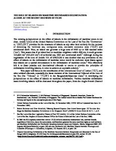


![Chapter 4 [PDF]](https://m.moam.info/img/260x300/chapter-4-pdf_5a03d8d01723dd07dc7774e9.jpg)


