2000, 74, 1–24
JOURNAL OF THE EXPERIMENTAL ANALYSIS OF BEHAVIOR
NUMBER
1 (JULY)
CHOICE IN A VARIABLE ENVIRONMENT: EVERY REINFORCER COUNTS M ICHAEL D AVISON
AND
W ILLIAM M. B AUM
UNIVERSIT Y OF AUCKLAND AND UNIVERSIT Y OF NEW HAMPSHIRE
Six pigeons were trained in sessions composed of seven components, each arranged with a different concurrent-schedule reinforcer ratio. These components occurred in an irregular order with equal frequency, separated by 10-s blackouts. No signals differentiated the different reinforcer ratios. Conditions lasted 50 sessions, and data were collected from the last 35 sessions. In Part 1, the arranged overall reinforcer rate was 2.22 reinforcers per minute. Over conditions, number of reinforcers per component was varied from 4 to 12. In Part 2, the overall reinforcer rate was six per minute, with both 4 and 12 reinforcers per component. Within components, log response-allocation ratios adjusted rapidly as more reinforcers were delivered in the component, and the slope of the choice relation (sensitivity) leveled off at moderately high levels after only about eight reinforcers. When the carryover from previous components was taken into account, the number of reinforcers in the components appeared to have no systematic effect on the speed at which behavior changed after a component started. Consequently, sensitivity values at each reinforcer delivery were superimposable. However, adjustment to changing reinforcer ratios was faster, and reached greater sensitivity values, when overall reinforcer rate was higher. Within a component, each successive reinforcer from the same alternative (‘‘confirming’’) had a smaller effect than the one before, but single reinforcers from the other alternative (‘‘disconfirming’’) always had a large effect. Choice in the prior component carried over into the next component, and its effects could be discerned even after five or six reinforcers into the next component. A local model of performance change as a function of both reinforcement and nonreinforcement is suggested. Key words: concurrent schedules, environmental variability, choice, generalized matching, contingency discriminability, key peck, pigeons
If individuals of a species could benefit by adapting their foraging strategies according to the amount of variation in the environment, then natural selection would favor such adaptation to variation. Research on the dynamics of foraging in variable environments has been relatively scant, with some noteworthy exceptions. Green (1980, 1984) argued that optimal foraging strategies ought to differ (be characterized by different rules) depending on the amount and pattern of patchto-patch variability. In particular, rules for leaving patches might change. Brunner, Kacelnik, and Gibbon (1996) tested this possi-
bility with starlings in an operant simulation of foraging and found that greater patch-topatch variability resulted in longer stays in the patches. The rules of patch leaving would reflect switching from one patch to another. If the alternatives of a concurrent schedule were considered patches, then a rule would reflect the pattern of switching or changing over between alternatives. The regularities of patch leaving are often called ‘‘rules of thumb,’’ because natural selection cannot produce literal optimizing, but may instead select rules that approximate optimality in the selecting environment. The idea of simple rules for patch leaving anticipates the possibility of dynamics, because some of the rules, particularly ones incorporating giving-up time (time since the last prey item) and run of bad luck (a series of failures to find food), imply a sensitivity to events as they occur. Behavioral ecologists discuss dynamics in connection with so-called ‘‘learning’’ rules. Two papers, by Krebs and Inman (1992) and Bernstein, Kacelnik, and Krebs (1988), speculate along this line. Both imagine a predator
This work was carried out at the University of Auckland and was supported by various grants to Michael Davison. We thank Mick Sibley who looked after the subjects and the masters and doctoral students who helped to conduct the experiment. A version of this paper was presented at the meeting of the Society for the Quantitative Analysis of Behavior, Orlando, Florida, May 1998. Reprints may be obtained from Michael Davison, Psychology Department, Auckland University, Private Bag 92019, Auckland, New Zealand (E-mail:
[email protected]) or William M. Baum, 611 Mason Street, #504, San Francisco, California 94108 (E-mail:
[email protected]). Raw data files may be obtained by sending a 100-MB zip disk to the former.
1
2
MICHAEL DAVISON and WILLIAM M. BAUM
wandering around in its environment, behaving in ways that can be described by simple rules and thereby generating a pattern of patch use. Such speculations might relate to the dynamics of choice in concurrent schedules. In the experimental analysis of behavior, the focus of research was initially on learning and how behavior changed over time. This was followed by a period in which the focus changed to the analysis of stable performance, and in this period many gains were made. In particular, for choice on concurrent schedules, Herrnstein (1961, 1970) formulated the strict matching law, which stated that the ratio of responses at two alternatives equaled (matched) the ratio of reinforcer frequencies obtained from the alternatives. Deviations from this relation led to its transformation into what has come to be called the generalized matching law (Baum, 1974): log
1B 2 5 a log1R 2 1 log c, B1
R1
2
2
(1)
where B1 and B2 refer to responses at Alternatives 1 and 2, and R1 and R2 refer to reinforcers obtained at Alternatives 1 and 2. The parameter a is called sensitivity to reinforcement (Lobb & Davison, 1975) and measures the change in log behavior ratio with a unit change in the log reinforcer ratio. The parameter c is bias and measures any constant preference to one alternative independent of the changes in the log reinforcer ratio. As Baum (1979) showed, Equation 1 is an excellent descriptor of stable performance under concurrent variable-interval (VI) schedules and some other concurrent schedules. With stable response ratios quantified this way, attention moved to behavioral transition, the way in which behavior changes from one stable state to another. There have been a number of approaches. For example, the behavioral effects of unpredictable step changes in reinforcer ratios have been investigated (Bailey & Mazur, 1990; Mazur, 1992; Mazur & Ratti, 1991). A more general approach attempted to drive the behavior–environment system with random variation in reinforcer ratios, seen as inputs akin to white noise (a pseudorandom binary sequence). Autocorrelation and related techniques have been used to extract the dependence of current
behavior ratios on sessional reinforcer ratios from the current and preceding sessions (Hunter & Davison, 1985; Schofield & Davison, 1997). Stable-state research on choice usually uses a stability criterion to determine when a transition has been completed and the new stable state has been reached (Killeen, 1978). Most such criteria report that stability is attained after about 15 or more hour-long sessions of training. However, research using pseudorandom binary sequences, in which the location of the two different concurrent schedules varied from session to session, revealed little contribution of reinforcer ratios in sessions more than three in the past (Hunter & Davison, 1985; see also Davison & Hunter, 1978). The results with these rapid step changes in reinforcer ratios imply that about 95% of asymptotic stability ought to be achieved in just three sessions on each new concurrent-schedule pair. Further research (Schofield & Davison, 1997) showed that continued exposure to concurrent schedules that change randomly from session to session may even eliminate any contribution of reinforcer ratios in sessions other than the present session. Such a result implies that transitions may be completed in a single session if subjects are adapted to rapidly changing environments. Indeed, Mazur (1992) and Mazur and Ratti (1991) documented large-scale changes in choice within single sessions in response to unpredictable changes in reinforcer ratios. The findings suggest that under conditions in which the reinforcing environment stays constant for long periods, behavioral adaptation to changes in the reinforcing environment might be slow, whereas when the reinforcing environment changes frequently, behavior might change rapidly. Such adjustment of behavioral change to frequency of environmental change would be adaptive and would make sense from the point of view of evolutionary theory. If the availability of resources in evolutionary niches was either always labile or always stable, then species might adapt to these situations. In some niches, however, the stability of resource availability might change often enough that selection could favor an even more efficient adaptation: the ability to adjust the speed of behavior transition to the frequency of change of the environment.
3
EVERY REINFORCER COUNTS The present research focused on the question: Will the pigeons’ choice ratios change more rapidly when the environment changes more frequently? We varied the speed of environmental change within sessions using a procedure introduced by Belke and Heyman (1994). A series of seven reinforcer ratios was arranged within each session. These components were not signaled, although the start of each new component was signaled by a preceding blackout. In Part 1, we investigated performance in components that lasted for 4, 6, 8, 10, and 12 reinforcers, asking whether sensitivity (a in Equation 1) was higher with shorter components. In Part 2, we arranged components that lasted for 4 or 12 reinforcers with six, rather than 2.22, reinforcers per minute arranged so as to investigate whether sensitivity to reinforcement in components was affected by changes in overall reinforcer rates. Such an effect has been reported for stable performance (Alsop & Elliffe, 1988). METHOD Subjects Six naive homing pigeons (numbered 91 to 96) were maintained at 85% 6 15 g of their free-feeding body weights. Water and grit were available at all times. Designated body weights were maintained by weighing the subjects and feeding amounts of mixed grain immediately after the final training session of the day. Apparatus The subjects were individually housed in cages (375 mm high by 370 mm deep by 370 mm wide) that also acted as the experimental chambers. On one wall of the cage were three plastic pecking keys (20 mm diameter) set 100 mm apart center to center and 220 mm from a wooden perch situated 100 mm from the wall and 20 mm from the floor. Each key could be transilluminated by yellow, green, or red light-emitting diodes, and responses to illuminated keys exceeding about 0.1 N were counted as effective responses. Beneath the center key and 60 mm from the perch was a magazine aperture (40 mm by 40 mm). During reinforcement, the keylights were extinguished, the aperture was illuminated, and the hopper, containing wheat, was raised for 2.5 s. The subjects could see and hear pi-
Table 1 Sequence of experimental conditions, number of reinforcers per component, the maximum number of reinforcers per session available, and the overall arranged rate of reinforcers in each condition of the experiment. In Conditions 4, 6, and 9, each component was presented twice per session.
Condition 1 2 3 (Rep C1) 4 5 6 7 8 9
Reinforcers per Reinforsession cers per (maxicomponent mum) 10 10 10 4 8 6 12 12 4
70 70 70 56 56 84 84 84 56
Reinforcers per minute 2.22 Varied 2.22 2.22 2.22 2.22 2.22 6 6
geons in other experiments, but no personnel entered the experimental room while the experiments were running. Procedure The subjects were slowly deprived of food by limiting their intakes. During this time, they were taught to eat from the food magazine when it was presented. When their weights approximated their designated weights and they were reliably eating during 2.5-s magazine presentations, they were autoshaped to peck the outer two response keys illuminated various colors. That is, one or the other key was illuminated for 4 s, and then food was presented independently of responding; if the pigeon pecked the illuminated key, food was presented immediately. When they were reliably pecking, they were then trained over 2 weeks on a series of reinforcement schedules increasing from continuous reinforcement to VI 30 s presented singly on the left and right keys with yellow keylights. They were then placed on the final procedure described below, but initially with the same, equal reinforcer rates on each key in each component. Sessions were conducted once per day, and commenced at the same time each day. The 6 subjects were studied in succession, with sessions lasting until a fixed number of reinforcers (see Table 1) had been collected or until 45 min had elapsed, whichever occurred first.
4
MICHAEL DAVISON and WILLIAM M. BAUM
Sessions commenced with the left and right keylights illuminated yellow, which signaled the availability of a VI schedule on each key. Sessions were divided into seven components, except in Conditions 4, 6, and 9, when 14 components were arranged. In the latter conditions, each of the basic seven components was first selected randomly, and then a second randomization of these components was arranged. Each component lasted for a fixed number of reinforcers (Table 1), and the components were separated by the blackout of both keys for 10 s. Apart from Condition 2, the arranged overall reinforcer rate was constant across components, but the values of the schedules on the two keys changed randomly over the components, providing seven different, unsignaled reinforcer ratios for the session. In all conditions, the reinforcer ratios in the seven components were 27:1, 9:1, 3:1, 1:1, 1:3, 1:9, and 1:27. Sessions ended with the extinguishing of both keylights. Condition 2 arranged a constant reinforcer rate (VI 27 s) on one key, and varied the reinforcer rate on the other key. These data were excluded from the analysis. In Conditions 1 to 7, we arranged 2.22 reinforcers per minute. Conditions 8 and 9 replicated Conditions 7 and 4, respectively, with six reinforcers per minute. A changeover delay (COD; Herrnstein, 1961) was in effect throughout. Following a changeover to either key, a reinforcer could not be obtained for responding at the key switched to until 2 s had elapsed from the changeover (i.e., the first response at the key). During sessions, the time of every event, coded by event type, was collected for detailed analysis. Training on each condition continued for 50 sessions, and the performances in the last 35 sessions were used in the data analyses. Condition 3 was a replication of Condition 1. RESULTS The first analysis investigated how log response ratios changed as a function of successive reinforcers delivered in each of the seven components. Figures 1 to 6 (individual subjects) and Figure 7 (group data) show these relations. To create these figures, all responses and time from the beginning of a
component to the first reinforcer were pooled across all 35 (or 70) presentations of the component, then all were pooled from the first reinforcer to the second, then from the second to the third, and so on. Thus the data were organized reinforcer by reinforcer, with performance measured prior to each reinforcer since the previous reinforcer or, for the first reinforcer of the component, since the beginning of the component (i.e., not cumulated across successive reinforcers). For all component lengths and both arranged reinforcer rates, response ratios changed with increasing number of reinforcers delivered in a fashion that was appropriate to the component reinforcer ratio. Figures 1 to 6, and particularly Figure 7, show a small effect of overall reinforcer rate: In components with unequal reinforcer ratios, response ratios changed more quickly and attained more extreme values when the reinforcer rate was six per minute than when it was 2.22 per minute. Also, for each arranged overall reinforcer rate, the curves associated with the different number of reinforcers per component were practically superimposable, although there may have been a slight tendency with 2.22 reinforcers per minute, but not with six reinforcers per minute, for preference to change faster for 10 and 12 reinforcers per component. The subsequent analyses categorized responses finely with respect to their occurrence in sequences of responses and reinforcers. Such fine-grained analyses require large pools of data to ensure that each category has a sufficient number of responses to generate reliable effects. Because of the high degree of consistency among the 6 pigeons that we have already demonstrated, we based subsequent data analyses on the data summed across subjects. Figure 8 shows fits of Equation 1 for log response ratios prior to each successive reinforcer versus arranged log reinforcer ratios for the group data obtained in Conditions 7 (2.22 reinforcers per minute) and 8 (six reinforcers per minute). Both conditions arranged 12 reinforcers per component. Equation 1 described the data well. Values of sensitivity to reinforcement (a in Equation 1) increased progressively from approximately zero prior to the first reinforcer to 0.52 (2.22 reinforcers per minute) and 0.63 (six rein-
EVERY REINFORCER COUNTS
5
Fig. 1. Bird 91. Log response ratios following each successive reinforcer delivered in each of the seven components in each condition of the experiment. Each panel shows data from a particular reinforcer ratio (indicated at the top of each panel). The different curves show data from conditions that arranged different numbers of reinforcers per component (R/C) and reinforcer rates (R/M) as indicated in the legend. Response numbers for each alternative were summed across all 35 sessions. On the x axis, the value of 0 indicates response ratios prior to the first reinforcer delivery.
forcers per minute). Figure 8 also shows that, except prior to the first reinforcer, sensitivity (a) was higher for the higher overall reinforcer rate. Table 2 shows the results of similar analyses done for all conditions and sub-
jects, and the same trends and differences are evident. Figures 9 (response allocation) and 10 (time allocation) show group estimates of sensitivity (a in Equation 1) for each condi-
6
MICHAEL DAVISON and WILLIAM M. BAUM
Fig. 2. Bird 92. Log response ratios as a function of successive reinforcers delivered in each of the seven components in each condition of the experiment. See Figure 1.
tion as a function of successive reinforcers in a component. Sensitivity increased from close to zero (often negative, particularly for time allocation) prior to the first reinforcer to values between 0.5 and 0.6 (2.22 reinforcers per minute) and 0.6 to 0.7 (six reinforcers per minute) after eight or nine reinforcers. The negative sensitivities prior to the first reinforcer may represent some carryover from
the prior component, which, because the first component would never be thus affected, would be more likely than not to have arranged a reinforcer ratio that favored the alternative response. Comparison across component durations at the fourth reinforcer in Figures 9 and 10 reveals that, for the lower rate of reinforcement, sensitivity increased as reinforcers per
EVERY REINFORCER COUNTS
7
Fig. 3. Bird 93. Log response ratios as a function of successive reinforcers delivered in each of the seven components in each condition of the experiment. One data point for the 27:1 reinforcer-ratio component fell off the graph. See Figure 1.
component increased from 4 to 12. No such difference appears for the higher rate of reinforcement. Either the effect of reinforcers per component was unreliable or it occurred only with the lower reinforcer rate. The degree to which preference in a previous component carried over into the next component is illustrated in Figures 11 (Con-
dition 7) and 12 (Condition 8). These figures show log response ratios as a function of successive reinforcers in both 1:1 and 27:1 reinforcer-ratio components according to the reinforcer ratio in the previous component. Because each component occurred only once per session (Table 1), a particular reinforcer ratio could never be followed by itself in Con-
8
MICHAEL DAVISON and WILLIAM M. BAUM
Fig. 4. Bird 94. Log response ratios as a function of successive reinforcers delivered in each of the seven components in each condition of the experiment. See Figure 1.
ditions 7 and 8. Although, because of small sample sizes, the variability was considerable, some clear trends may be seen. First, the preferences converged with successive reinforcers, resembling Figures 1 to 7. Second, performance prior to Reinforcer 1 in a component depended on the reinforcer ratio in the previous component. Third, this response-rate differential probably lasted for
three or four reinforcers. The analyses shown in Figures 1 to 7 and in Figures 8 and 9 obscured this carryover effect by averaging across the differing prior-component reinforcer ratios. Further analyses reported below will more completely analyze these carryover effects. Is performance in a component prior to the first reinforcer the same as performance
EVERY REINFORCER COUNTS
9
Fig. 5. Bird 95. Log response ratios as a function of successive reinforcers delivered in each of the seven components in each condition of the experiment. Two data points for the 1:27 reinforcer-ratio component fell off the graph. See Figure 1.
at the end of the previous component, or did some preference attenuation occur over the 10-s blackout? To answer this question, we plotted the log response ratio before the first reinforcer in a component against the log response ratio obtained between the final two reinforcers in the previous component. Figure 13 shows the group results for Conditions
3 to 7. Straight lines were fitted to these scatter plots (N 5 approximately 1,260). If preference following the blackout were the same as preference before the blackout, the slopes of the regression lines in Figure 13 would equal 1.0. The obtained slopes ranged from 0.12 to 0.16, and were unrelated to the number of reinforcers in a component. The flat-
10
MICHAEL DAVISON and WILLIAM M. BAUM
Fig. 6. Bird 96. Log response ratios as a function of successive reinforcers delivered in each of the seven components in each condition of the experiment. See Figure 1.
ness of these slopes suggests that log response ratios might tend to regress towards indifference during the blackout. Figure 14 shows that similar analyses for Conditions 8 and 9 (six reinforcers per minute) produced slopes of 0.16 and 0.12, within the range obtained for 2.22 reinforcers per minute. Thus, neither number of reinforcers per component
nor overall reinforcer rate affected the degree of regression towards indifference. Local Analysis A more detailed analysis examined response ratios in the interreinforcer intervals after various sequences of reinforcers. It began with the response ratio at the beginning
EVERY REINFORCER COUNTS
11
Fig. 7. Group log response ratios obtained by summing response numbers over the 6 subjects as a function of successive reinforcers delivered in each of the seven components in each condition of the experiment. See Figure 1.
of a component, up to the first reinforcer. After the first reinforcer and before the second reinforcer, two response ratios were calculated, one following a reinforcer on the left and the other following a reinforcer on the right. After the second reinforcer and before the third reinforcer, four response ratios were calculated, one for each of the four sequences of two reinforcers: left-left, left-right, right-
right, and right-left. These sequences came from various component reinforcer ratios, although the frequency with which each sequence occurred varied with the component reinforcer ratios (e.g., a series of several reinforcers on the left would rarely occur in the 1:27 component). Figure 15 shows this analysis for the grouped data up to the response ratios between the third and fourth reinforc-
12
MICHAEL DAVISON and WILLIAM M. BAUM
Fig. 8. Group log response ratios in Conditions 7 (12 reinforcers per component, 2.22 reinforcers per minute) and 8 (12 reinforcers per component, six reinforcers per minute) as a function of the arranged log reinforcer ratio in the components for the data collected before the first reinforcer (R1), between the first and second reinforcers (R2), up to the 12th reinforcer. Filled circles show data from Condition 7, and open circles show data from Condition 8.
13
EVERY REINFORCER COUNTS Table 2 Values of sensitivity (a) and bias (log c) for each experimental condition prior to each successive reinforcer in the components. The data used were averaged over the 6 subjects (i.e., the response and reinforcer totals were averaged and sensitivity values were determined from those averages). Reinforcer number Parameter 1 2 3 4 5 6 7 8 9 10 11 12
a log a log a log a log a log a log a log a log a log a log a log a log
c c c c c c c c c c
Condition 1
3
5
6
7
8
9
20.06 20.01 0.19 0.01 0.27 0.03 0.34 0.03 0.37 0.02 0.40 0.01 0.44 0.02 0.44 0.04 0.44 0.03 0.44 0.01
20.03 0.02 0.16 0.02 0.24 0.03 0.30 0.02 0.37 0.04 0.39 0.03 0.41 0.06 0.43 0.08 0.44 0.06 0.47 0.06
20.02 20.02 0.16 20.00 0.26 20.02 0.31 20.00 0.35 20.01 0.36 0.02 0.39 0.01 0.40 20.00
20.01 20.03 0.17 20.01 0.26 20.02 0.29 0.00 0.34 20.00 0.38 0.00
20.03 20.04 0.18 0.04 0.29 0.04 0.37 0.03 0.41 0.05 0.46 0.02 0.50 0.03 0.49 0.02 0.48 0.03 0.47 0.03 0.49 0.03 0.52 20.01
20.02 20.07 0.21 20.03 0.38 0.01 0.44 20.00 0.50 20.01 0.54 20.00 0.62 20.01 0.60 20.01 0.64 0.00 0.63 20.03 0.61 20.01 0.63 0.00
20.00 20.08 0.26 20.03 0.39 20.02 0.43 20.04
c c
ers. The result appears as a branching tree. The average log response ratio before the first reinforcer, corresponding to 0 on the x axis, was close to zero, indicating no average preference at the beginning of the component. The various response ratios that occurred as carryovers from the previous components, shown in Figures 11 and 12, approximately canceled one another out. Each successive reinforcer produced a shift of preference (log response ratio) toward the alternative from which it came. When all three reinforcers occurred on the left or the right, preference shifted consistently toward the left or right. Whenever a shift of reinforcer source occurred, a shift in preference followed it. The effects of each successive reinforcer decreased as more reinforcers were delivered without a change in source, as indicated by the curvature of the outermost branches. The greater spread of the two trees for the higher reinforcer-rate conditions indicates that preference shifted more with successive reinforcers with the higher than with
the lower reinforcer rate. Number of reinforcers per component appeared to have no consistent effect, although 12 reinforcers per component showed a little more reinforcer effect than did the other conditions. This difference disappeared with the higher reinforcer rate, however. Figure 16 shows more of the tree structure, focusing on single right (or left) ‘‘disconfirming’’ reinforcers at sequential positions up to the eighth reinforcer. We shall call such a reinforcer a disconfirmation. All disconfirmations moved performance toward the alternative from which the reinforcer came. Although the effects of successive confirmations decreased, the effects of disconfirmations tended to increase across successive reinforcers; the later in the sequence that a disconfirming reinforcer occurred, the more it drew preference toward its source. If the disconfirmation occurred after about the fourth reinforcer, it moved preference to approximate indifference. The results for other conditions resembled those in Figure 16.
14
MICHAEL DAVISON and WILLIAM M. BAUM
Fig. 9. Response-allocation sensitivity to reinforcement (from fits exemplified in Figure 8) according to Equation 1 for the group average data (response numbers summed over all 6 subjects) as a function of successive reinforcers delivered in all conditions of the experiment. R/C indicates the number of reinforcers per component, and Hi indicates the conditions in which six (rather than 2.22) reinforcers per minute were arranged.
Fig. 11. Condition 7 (2.22 reinforcers per minute). Log response ratios in 1:1 and 27:1 reinforcer-ratio components as a function of successive reinforcers delivered according to the reinforcer ratio in the previous component, as shown on the legend. The results from the first component of a session, which did not follow any other component, are labeled ‘‘first component.’’
The contributions of the reinforcer ratio in the previous component (carryover sensitivity) and of the reinforcer ratio in the present component (current-component sensitivity) on preference in the present component may be assessed by the use of multiple linear regression. The equation for this analysis was log Fig. 10. Time-allocation sensitivity to reinforcement (from fits exemplified in Figure 8) according to Equation 1 for the group average data (times summed over all 6 subjects) as a function of successive reinforcers delivered in all conditions of the experiment. R/C indicates the number of reinforcers per component, and Hi indicates the conditions in which six (rather than 2.22) reinforcers per minute were arranged.
R lp Bli R 5 api log 1 aci log lc 1 log c, Bri R rp R rc
(2)
where B and R refer to responses and arranged component reinforcers, l and r refer to the left and right alternatives, p and c refer to the previous and current components, and i is the reinforcer order in a component (i 5 0, prior to the first reinforcer, to one less than
EVERY REINFORCER COUNTS
Fig. 12. Condition 8 (six reinforcers per minute). Log response ratios in 1:1 and 27:1 reinforcer-ratio components as a function of successive reinforcers delivered according to the reinforcer ratio in the previous component, as shown on the legend. The results from the first component of a session, which did not follow any other component, are labeled ‘‘first component.’’
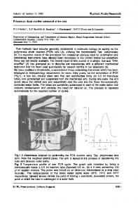
the number of reinforcers per component). This equation was fitted to the response ratios for each successive reinforcer averaged across subjects. The results appear in Figure 17. Sensitivity to the previous component reinforcer ratio (api) always started above zero, and fell progressively towards zero as more reinforcers were delivered. The starting sensitivity increased from about 0.1 for four reinforcers per component to about 0.3 for 12 reinforcers per component, reflecting the dependence of the response ratio at the end of the previous component on the number of reinforcers (Figures 1 to 7). Sensitivity to the current reinforcer ratio started from slightly below zero (reflecting the probability that the
15
prior component arranged an opposing reinforcer ratio) and increased to about 0.5 to 0.6 for 2.22 reinforcers per minute and to 0.7 to 0.8 for six reinforcers per minute. The difference between the final sensitivity to the current reinforcer ratio and the starting sensitivity to the previous reinforcer ratio shows the effect of the intercomponent blackout. The blackout had a large effect on response allocation, often nearly halving sensitivity from the end of one component to the beginning of the next. The proportional decrease due to the blackout was larger for fewer reinforcers per component and for the higher reinforcer rate. Comparison of the top two graphs and the bottom two graphs reveals that current-component sensitivities for six reinforcers per minute were reliably higher than those for 2.22 reinforcers per minute after the first reinforcer delivery, but there were no clear differences in the sensitivity to the previous-component reinforcer ratios. As in Figures 9 and 10, sensitivity at the fourth reinforcer was lower for the four reinforcers per component than for the 12 reinforcers per component, but only for the lower rate of reinforcement. The current-component sensitivities shown in Figure 17 generally exceed those in Figure 9. The reason is that the analyses of Figure 9 took no account of carryover from the previous component. Because of the greater probability that the previous component entailed a preference opposite to the current component, carryover tended to decrease current-component sensitivity in Figure 9. When carryover was quantitatively removed in Figure 17, current-component sensitivity tended to increase. Figure 17 also summarizes carryover effects like those shown in Figures 11 and 12 with the effects of the current-component reinforcer ratio eliminated. DISCUSSION The present results show that there are situations in which behavioral adjustment occurs very rapidly—much faster than is implied by the usual requirement of 15 to 30 hour-long sessions to attain stable molar performance. However, the adjustment appears to be incomplete, in the sense that the asymptotic sensitivities obtained in the present
16
MICHAEL DAVISON and WILLIAM M. BAUM
Fig. 13. Scatterplots of the relation between log response ratios emitted before the first reinforcer in a component as a function of the log response ratio emitted before the final reinforcer of the previous component. The lines, and associated equations shown on the graphs, show the best fitting linear regressions through the data. The data are from conditions that arranged 2.22 reinforcers per minute.
EVERY REINFORCER COUNTS
17
Fig. 14. Scatterplots of the relation between log response ratios emitted before the first reinforcer in a component as a function of the log response ratio emitted before the final reinforcer of the previous component. The lines, and associated equations shown on the graphs, show the best fitting linear regressions through the data. The data are from conditions that arranged six reinforcers per minute.
experiment after 8 to 12 reinforcers (Figures 9 and 17) fall short of those obtained in steady-state experiments (Baum, 1979; Taylor & Davison, 1983). At present, we have no obvious mathematical description of the change in sensitivity with increasing numbers of reinforcers that might allow us to predict the asymptotic sensitivity. We examined several candidate functions—exponential, hyperbolic, Rescorla-Wagner, and others—but none seemed better than any other. Indeed, most of these predict steady-state asymptotes little higher than the sensitivity obtained here after 8 to 12 reinforcers. Is the high frequency of change in reinforcer ratios causing a lower-than-usual steady-state asymptote? If so, we would expect some change in performance as reinforcers per component increased from 4 to 12. However, the most detailed analysis of the present data (Figure 17) showed no such change. Instead, Figure 17 showed that the curves from the different conditions were superimposable, as in Figure 9, and that carryover between components had no effect on asymptotic sensitivity. If the frequency of changing reinforcer ratios affects asymptotic sensitivity,
the effect is small across the range of reinforcers per component that we investigated. The increase in adjustment speed with overall reinforcer rate, shown most clearly in Figures 7 and 9, resembles the increase in steady-state sensitivity with overall reinforcer rate reported by Alsop and Elliffe (1988) and by Elliffe and Alsop (1996). Because the steady-state relations between sensitivity and reinforcer rate were sometimes nonmonotonic, however, and the present experiment included only two different rates, the correspondence remains to be investigated in more detail. The present results suggest that any model of transition should accommodate increase in sensitivity with increase in overall reinforcer rate. Figure 15 shows that, following a reinforcer from one source, two reinforcers from the other source moved preference close to the trajectory for three reinforcers from only that second source. This suggests that at least a few reinforcers are required to shift preference following an unsignaled change in reinforcer ratio. In the present experiment, however, the onset of a new reinforcer ratio was preceded by a blackout. Figure 17 shows
18
MICHAEL DAVISON and WILLIAM M. BAUM
Fig. 15. Log response ratios following each reinforcer delivery in sequences of left- and right-key reinforcer deliveries for all conditions of the experiment. For clarity, only the data up to the delivery of the third reinforcer are shown. Dotted lines join points in which right reinforcers were subsequently delivered.
EVERY REINFORCER COUNTS
19
A Model The model is a local model in the sense that it considers the behavior change produced by reinforcement and nonreinforcement. Its logic is based on the concurrentschedule model offered by Davison and Jenkins (1985), in which the discriminability of response–reinforcer relations (dr) determines the effects of delivered reinforcers on the alternative responses. It is a cumulativeeffects model (Davis, Staddon, Machado, & Palmer, 1993) because the effects of reinforcers are accumulated, via the response–reinforcer discrimination process, to the two alternatives. It is also an allocation model in relation to the effects of nonreinforcement, which is assumed both to decrease and to mix the allocated reinforcer counts to the two alternatives. Three processes are assumed. The first process allocates each reinforcer to the two response-related accumulations according to Equations 3a and 3b. For the ith reinforcer delivery, which may be on the left (Rl,i) or right (Rr,i) alternative,
Fig. 16. Log response ratios following selected sequences of left-right reinforcer deliveries in Conditions 7 (2.22 reinforcers per minute) and 8 (six reinforcers per minute) when 12 reinforcers per component were arranged. The sequences were L, LR, LLR, LLLR, etc., and R, RL, RRL, RRRL, etc. Dotted lines join disconfirmations, in which a reinforcer was delivered for a response on an alternative that was different from prior reinforced responses in that component.
that the 10-s blackouts acted as signals because they substantially reduced preference. Any mathematical model of these data must account for four effects: (a) the reduction in preference during blackout; (b) the decreasing effects of continued reinforcers from the same source (Figures 15 and 16); (c) the strong effects of changes in the source; and (d) the increase in sensitivity with increasing overall reinforcer rate (Figure 17). We now offer a model based on this reasoning.
ˆ l,i 5 R ˆ l,i21 1 pd R l,i 1 (1 2 pd )R r,i , R
(3a)
and ˆ r,i 5 R ˆ r,i21 1 pd R r,i 1 (1 2 pd )R l,i , R
(3b)
where either Rl,i 5 1 and Rr,i 5 0, or vice ˆ is the reinforcer accumulation prior versa. R to (subscript i 2 1) and after (subscript i) reinforcer i. The response–reinforcer discriminability parameter, pd, determines the frequency with which a delivered reinforcer is allocated to the just-emitted response or to the alternative response. When a reinforcer is delivered, if pd equals .5 (the response–reinforcer relations are indiscriminable), then on average half of each reinforcer will be allocated to each of the responses. If pd equals 1.0 (perfect discrimination), then each reinforcer will be completely allocated to the response that produced it. Because a value of pd less than 1.0 applies only to experiments in which the response alternatives are imperfectly discriminated (e.g., Davison & Jones, 1995; Davison & Nevin, 1999; Miller, Saunders, & Bourland, 1980), and the present procedure ensured that the alternatives should be highly discriminable, we will assume that
20
MICHAEL DAVISON and WILLIAM M. BAUM
Fig. 17. Sensitivity to reinforcement values from multiple linear regressions between log response ratios and arranged log reinforcer ratios (Equation 2) in the previous and the present components for each successive reinforcer delivery. R/C indicates the number of reinforcers per component, and Hi indicates the conditions in which six reinforcers per minute were arranged.
EVERY REINFORCER COUNTS pd equals 1.0 for the purposes of the present analysis. Equations 3a and 3b accomplish the accumulation of reinforcer effects implied by the growing preferences shown in Figures 1 through 7 and by the growth in sensitivity shown in Figures 9 and 17. The successive application of Equations 3a and 3b leads to increasing allocations of reinforcers to two response alternatives and, assuming that response ratios equal allocated reinforcer ratios, to strict matching (when pd 5 1) or to undermatching (when pd , 1). However, the increases in allocations are without limit. Two further mechanisms must be postulated both to limit reinforcer accumulations and to deal with other changes demonstrated in the present data. First, the persistent malleability of preference suggests a role for the passage of time. We assume that as events recede into the past they become less efficacious in controlling current behavior. Without some mechanism for past reinforcers to lose effect with time, preference would become increasingly insensitive to change in reinforcer ratio because accumulations would become infinitely large. One way to maintain the sensitivity of behavior to changing reinforcer frequencies on the alternatives is to allow the effects of accumulated reinforcers to ebb over time. If reinforcer accumulations are low, current reinforcers can exert more effect on preference. Second, we found that preference regressed toward indifference during the 10-s blackouts between components (Figure 17). Loss of accumulated reinforcers, on its own, cannot satisfy this second requirement. To describe the regression of preference during blackout, accumulations of reinforcers to alternatives have to become progressively less differential during blackout—the accumulations should leak into each other. These additional processes—loss of reinforcers and loss of reinforcer differential—which tend to undo the first process of accumulation (Equations 3a and 3b), are embodied in the following equations: ˆ l,t 5 pD pe R ˆ l,i21 1 (1 2 pD )pe R ˆ r,t21, (4a) R and ˆ r,t 5 pD pe R ˆ r,t21 1 (1 2 pD )pe R ˆ l,t21. R
(4b)
Equations 4a and 4b are difference equations to be applied at the end of every (arbitrary)
21
ˆ is the reinforcer fixed time epoch. Again, R accumulation prior to (subscript t 2 1) and after (subscript t) the end of the epoch. The values of the parameters pD and pe depend on the epoch duration chosen. At the end of each time epoch, both during the intercomponent blackout and during the components, some reinforcers accumulated in the last ˆ l,t21 and (1 2 pe)R ˆ r,t21] component [(1 2 pe)R are lost. The parameter pe is thus interpreted as a discriminability parameter between the arranged reinforcers and the extraneous reinforcers (e.g., Herrnstein, 1970). We will call it arranged–extraneous discriminability. If pe 5 .5, half of the accumulated reinforcers are lost at each time slice, whereas if it equals 1.0, none are lost. To explain absolute response rates using this model, extraneous sources of reinforcement should also be incorporated into the equations. Because, however, such a process is difficult to model, we will make no attempt here. Also, at the end of each epoch, the accumulated reinforcers for the alternatives are reallocated between the alternatives according to the value of pD, accumulation discriminability. If pD 5 .5, reinforcer allocations would equalize in a single epoch. If it equals 1.0, then no reallocation would occur. To describe the present data, pD must lie between these two extremes. This reallocation process means that higher overall reinforcer rates will give greater sensitivity, because of less reallocation of reinforcer accumulations via pD between reinforcers. Because we assume that this process also occurs during the blackout between components, we expect that longer blackouts will produce both less carryover between components (via pD) and faster shifts in preference at the start of components (because, via pe, more reinforcers allocated to the alternatives would be lost during the blackout). These effects will be investigated in subsequent research. Equations 3 and 4 together provide two sources of undermatching (Baum, 1974). One would occur on reinforcer input (via pr) if response alternatives were imperfectly discriminated, and one occurs on nonreinforcement (via pD). Both of these processes may be necessary for a complete account of concurrent performance. Baum, Schwendiman, and Bell (1999) showed that molar contingency discriminability (Alsop, 1991; Davison, 1991; Davison & Jenkins, 1985; Davison &
22
MICHAEL DAVISON and WILLIAM M. BAUM
Fig. 18. Predictions of sensitivity to reinforcement values obtained from a simulation of the model embodied in Equations 3 and 4. The figure parallels Figure 17.
Jones, 1995, 1998) fails to describe the full extent of undermatching on typical concurrent VI VI schedules. The addition of the pD process allows asymptotic choice to undermatch reinforcer ratios even when we expect the alternatives to be perfectly discriminated (pr 5 1.0), as in the present experiment. Figure 18 shows a representative set of predictions from this model, simulating some of the data shown in Figure 17. Sensitivity (to both current-component and previous-component reinforcer ratios) changes appropriately with increasing numbers of delivered reinforcers. Equations 3 and 4 together constitute a local model of concurrent-schedule performance. It might seem to be contradicted by standard experiments on concurrent VI VI schedules, in which the time between components is usually on the order of 23 hr, and one might expect that, according to the model, each session would commence with equal response allocation between alternatives. No such regression to indifference occurs, because the blackout functions differently in a steady-state situation compared with the situation investigated here. In usual steady-state concurrent VI VI experiments, the delay between components (i.e., sessions) usually signals no change, whereas in the present experiment it signaled that a different reinforcer ratio would follow. In the usual experiment, no ‘‘directed forgetting’’ should
occur, as it does here, so we expect attenuated pe and pD effects in the standard experiment. This line of speculation is supported by the observation that regression toward indifference occurs between sessions early after steady-state transitions (Hunter, 1979; Mazur, 1996), consistent with our model. In situations in which reinforcer ratios change randomly between sessions, with the usual 23-hr delay (Hunter & Davison, 1985; Schofield & Davison, 1997), previous sessions’ reinforcer ratios affect current response ratios, but response ratios change rapidly at the start of each new session. Indeed, prolonged exposure to random changes between sessions (Schofield & Davison, 1997) decreases carryover between sessions, implying enhanced directed forgetting between sessions. All these findings support the present model. Further, the present model predicts exclusive preference on concurrent VI extinction, but only if pr and pD both equal 1.0; if either is less than 1.0, some responding will continue at the extinction alternative (Baum et al., 1999; Davison & Jones, 1998). The present procedure revealed processes that are invisible to steady-state research. Even experiments that arrange step changes in reinforcer ratio (Bailey & Mazur, 1990; Mazur, 1992; Mazur & Ratti, 1991) reveal little of the way in which these relatively local processes govern transition between steady states. The present procedure allowed us to analyze a large number of transitions among seven different reinforcer ratios and to extract the essential features of these transitions. It also amplified the effects of individual reinforcers and reinforcer sequences (Figure 16) in comparison with steady-state performance, in which averaging obscures these effects. In terms of our model, steady-state experiments produce reinforcer accumulations that are high and constant after long exposure to a fixed reinforcer ratio; the effects of additional reinforcers would be negligible. Perhaps the most striking result was, within the range investigated, the absence of any major effect of reinforcers per component. Figures 9, 10, and 17 show a small effect of from 4 to 12 reinforcers per component for the lower overall reinforcer rate. However, no such effect appeared for the higher overall reinforcer rate, and even for the lower rate, it was probably negligible; the differences in
EVERY REINFORCER COUNTS sensitivity generally fell short of 0.1, only coming up to 0.1 in the performance between the third and fourth reinforcers. The main result was that change in preference with successive reinforcer deliveries in components was rapid, with sensitivity reaching high levels after only six to eight reinforcers. The strong regularities in the sequential effects of reinforcer source (Figures 15 and 16) indicate that preference was controlled at a local level. Although each reinforcer had an effect, as the number of reinforcers increased in a component, the effect of each additional confirming reinforcer decreased, indicating some process of accumulation, such as that described in Equation 3. However, the effect of disconfirming reinforcers increased with successive reinforcers, indicating that accumulated reinforcers leaked at a high rate (large pe). At the same time, the carryover effects of reinforcers delivered in the previous component progressively decreased with reinforcers delivered in the next component (Figures 11, 12, and 17). This decrease was modeled by assuming that prior accumulations reallocate between choice alternatives during periods of nonreinforcement (Equation 4). The resulting model, which is a dynamical alternative to molar and molecular maximizing and to melioration, seems viable. Subsequent research will test it further. REFERENCES Alsop, B. (1991). Behavioral models of signal detection and detection models of choice. In M. L. Commons, J. A. Nevin, & M. C. Davison (Eds.), Signal detection: Mechanisms, models, and applications (pp. 39–55). Hillsdale, NJ: Erlbaum. Alsop, B., & Elliffe, D. (1988). Concurrent-schedule performance: Effects of relative and overall reinforcer rate. Journal of the Experimental Analysis of Behavior, 49, 21–36. Bailey, J. T., & Mazur, J. E. (1990). Choice behavior in transition: Development of preference for the higher probability of reinforcement. Journal of the Experimental Analysis of Behavior, 53, 409–422. Baum, W. M. (1974). On two types of deviation from the matching law: Bias and undermatching. Journal of the Experimental Analysis of Behavior, 22, 231–242. Baum, W. M. (1979). Matching, undermatching, and overmatching in studies of choice. Journal of the Experimental Analysis of Behavior, 32, 269–281. Baum, W. M., Schwendiman, J. W., & Bell, K. E. (1999). Choice relations in the extreme: Matching, contingency discrimination, and foraging theory. Journal of the Experimental Analysis of Behavior, 71, 355–373. Belke, T. W., & Heyman, G. M. (1994). Increasing and
23
signaling background reinforcement: Effect on the foreground response-reinforcer relation. Journal of the Experimental Analysis of Behavior, 61, 65–81. Bernstein, C., Kacelnik, A., & Krebs, J. R. (1988). Individual decisions and the distribution of predators in a patchy environment. Journal of Animal Ecology, 57, 1007–1026. Brunner, D., Kacelnik, A., & Gibbon, J. (1996). Memory for inter-reinforcement interval variability and patch departure decisions in the starling, Sternus vulgaris. Animal Behaviour, 51, 1025–1045. Davis, D. G. S., Staddon, J. E. R., Machado, A., & Palmer, R. G. (1993). The process of recurrent choice. Psychological Review, 100, 320–341. Davison, M. (1991). Stimulus discriminability, contingency discriminability, and stimulus generalization. In M. L. Commons, J. A. Nevin, & M. C. Davison (Eds.), Signal detection: Mechanisms, models, and applications (pp. 57–78). Hillsdale, NJ: Erlbaum. Davison, M. C., & Hunter, I. W. (1978). Concurrent schedules: Undermatching and control by previous experimental conditions. Journal of the Experimental Analysis of Behavior, 32, 233–244. Davison, M., & Jenkins, P. E. (1985). Stimulus discriminability, contingency discriminability, and schedule performance. Animal Learning & Behavior, 13, 77–84. Davison, M., & Jones, B. M. (1995). A quantitative analysis of extreme choice. Journal of the Experimental Analysis of Behavior, 64, 147–162. Davison, M., & Jones, B. M. (1998). Performance on concurrent variable-interval extinction schedules. Journal of the Experimental Analysis of Behavior, 69, 49– 57. Davison, M., & Nevin, J. A. (1999). Stimuli, reinforcers, and behavior: An integration. Journal of the Experimental Analysis of Behavior, 71, 439–482. Elliffe, D., & Alsop, B. (1996). Concurrent choice: Effects of overall reinforcer rate and the temporal distribution of reinforcers. Journal of the Experimental Analysis of Behavior, 65, 445–463. Green, R. F. (1980). Bayesian birds: A simple example of Oaten’s stochastic model of optimal foraging. Theoretical Population Biology, 18, 244–256. Green, R. F. (1984). Stopping rules for optimal foragers. The American Naturalist, 123, 30–40. Herrnstein, R. J. (1961). Relative and absolute strength of response as a function of frequency of reinforcement. Journal of the Experimental Analysis of Behavior, 4, 267–272. Herrnstein, R. J. (1970). On the law of effect. Journal of the Experimental Analysis of Behavior, 13, 243–266. Hunter, I. W. (1979). Static and dynamic models of concurrent variable-interval schedule performance. Unpublished doctoral dissertation, University of Auckland. Hunter, I., & Davison, M. (1985). Determination of a behavioral transfer function: White-noise analysis of session-to-session response-ratio dynamics on concurrent VI VI schedules. Journal of the Experimental Analysis of Behavior, 43, 43–59. Killeen, P. R. (1978). Stability criteria. Journal of the Experimental Analysis of Behavior, 29, 17–25. Krebs, J. R., & Inman, A. J. (1992). Learning and foraging: Individuals, groups, and populations. The American Naturalist, 140, S63–S84. Lobb, B., & Davison, M. C. (1975). Performance in concurrent interval schedules: A systematic replication.
24
MICHAEL DAVISON and WILLIAM M. BAUM
Journal of the Experimental Analysis of Behavior, 24, 191– 197. Mazur, J. E. (1992). Choice behavior in transition. Journal of Experimental Psychology: Animal Behavior Processes, 18, 364–378. Mazur, J. E. (1996). Past experience, recency, and spontaneous recovery in choice behavior. Animal Learning & Behavior, 24, 1–10. Mazur, J. E., & Ratti, T. A. (1991). Choice behavior in transition: Development of preference in a free-operant procedure. Animal Learning & Behavior, 19, 241– 248. Miller, J. T., Saunders, S., & Bourland, G. (1980). The
role of stimulus disparity in concurrently available reinforcement schedules. Animal Learning & Behavior, 8, 635–641. Schofield, G., & Davison, M. (1997). Nonstable concurrent choice in pigeons. Journal of the Experimental Analysis of Behavior, 68, 219–232. Taylor, R., & Davison, M. (1983). Sensitivity to reinforcement in concurrent arithmetic and exponential schedules. Journal of the Experimental Analysis of Behavior, 39, 191–198. Received April 30, 1999 Final acceptance March 12, 2000