The finite volume (FV) method starts with the integral form of a conservation ... the
main reason for using unstructured FV methods is precisely that they can be ...
MSc. Advanced CFD (2011)
1
Finite Volume Methods for Unstructured Grids
1.1
Introduction
The finite volume (FV) method starts with the integral form of a conservation equation: � � � � ∂ ρ φ dΩ + ρ φ v.n dS = ρ γ (grad (φ) .n )dS + qφ dΩ ∂t Ω S S Ω
(1)
and is obtained by integrating: ∂ρφ + div(v ρ φ) = div(ρ γgrad (φ)) + qφ ∂t
(2)
over any control volume Ω bounded by the surface S, on which n is the normal directed toward the outside of Ω. The integral conservation equation (1) is valid for any control volume Ω. It is applied to every cell of the mesh. These cells usually consist of rectangles or triangles in 2D, and hexahedra, prisms, or tetrahedra in 3D. More generally, any type of volume, bounded by Ns planar surfaces, is possible.
Hexahedra, Prisms, and Tetrahedra The control volumes (CV) are noted Ti (considering Triangles as generic examples), the union of all CV (i = 1, .., NCV ) forming a partition of the entire flow domain. The surface integrals appearing in (1) when applied to the CV Ti is simply the sum of fluxes over the number N s of planar surfaces separating Ti from the neighbour cells: � � � ρ φ v.n dS = ρ φ v.n dS Ti
j=1,Ns
Sij
� � The contribution Sij ρ φ v.n dS in the summation j=1,N s is the flux of the quantity ρ φ carried by the flow velocity v across the surface Sij between cells i and j. For cell P in figure 1, this writes: � � div(v ρ φ)dS = ρ φ v.n dS cell P surf ace cell P � � � � = ρ φ v.n dS + ... + ... + ... SP E
SP N
SP W
SP S
The calculation for one interfacial surface Sij between cell i and cell j needs to be described only once, even though it will appear again when computing the fluxes into cell j. Indeed only the direction of the external normal is reversed, thus � only the sign of the flux needs to be exchanged. For example on fig 1, the absolute value of flux SP E ρ φ � v.nP E � dSj across the boundary between the quadrangle centred on P and the triangle centred on E must be calculated only once, then it contributes to cell P with a + sign if v.nP E . > 0 if v is pointing out of P ( nP E is pointing to the exterior of cell P). When considering cell E, the same expression will appear except that now nEP is pointing to the exterior of cell E toward cell P hence a - sign is affected to the absolute flux if v.nEP . < 0 . 1
N n
nw
ne W
E P
sw
se
Figure 1: Combination of rectangular and triangular CV
S i-1/2 i-1
n
S i+1/2 u i
n
u i+1
Figure 2: 1D convection problem This is what makes the method absolutely conservative, for mass, momentum and scalars, however coarse the mesh. It is of course very appealing for industrial calculations where mesh refinement is not always possible. However it is quite difficult to evaluate φ at the interface, since one knows only the average values φP and φE as is explained further. This step is often (hardly!) first order accurate on strongly distorted meshes. (It is usually quite accurate on regular meshes, i.e. second order, but the main reason for using unstructured FV methods is precisely that they can be applied to very complex geometries, where the mesh generators usually produce quite distorted cells)
1.2
1D example
The issues of FV against FD can be first outlined on the following 1D example of convection in a pipe with variable section as shown in figure 2. ∂φ + div(v φ) = 0 (3) ∂t In 1D the velocity vector is simply v = (u, 0, 0) where u is assumed constant, then v n = u if n is pointing to the right and −u otherwise. Let Ω the control volume centred on node i and bounded by surfaces Si+1/2 , Si−1/2 . The FV
2
formulation is then: � � i � Si+1/2 + Si−1/2 ∂ ∂φ � φ dΩ + φ.v n dS = xi+1/2 − xi−1/2 ∂t Ω ∂t 2 S � � � � + φ xi+1/2 Si+1/2 (v n)i+1/2 + φ xi−1/2 Si−1/2 (v n)i−1/2
(4) (5)
This formula would be valid for a pipe with variable section. For simplicity let us assume the sections constant and equal to unity. Then: i
� � � � � �� ∂φ � xi+1/2 − xi−1/2 + u φ xi+1/2 − φ xi−1/2 = 0 ∂t
note that (v n)i+1/2 = +u , while (v n)i−1/2 = −u and Si+1/2 = Si−1/2 = 1. Furthermore we have defined the average value of φ inside the CV as: � xi+1 /2 1 i � φ =� φ.dx (6) xi+1/2 − xi−1/2 xi−1/2 One could also introduce the average value of the derivative: � � � � i � xi+1 /2 φ xi+1/2 − φ xi−1/2 ∂φ dφ 1 � � � dx = =� ∂x xi+1/2 − xi−1/2 xi−1/2 dx xi+1/2 − xi−1/2
Then the FV formulation can be seen as: � i i i � � ∂φ � � � � � � �� ∂φ ∂φ +u xi+1/2 − xi−1/2 = xi+1/2 − xi−1/2 + u φ xi+1/2 − φ xi−1/2 ∂t ∂x ∂t
(7)
(8)
This is not an � approximation,� but an exact representation of the physical process occurring within the segment xi+1/2 − xi−1/2 centred around node xi . However several approximations will need to the introduced: � � • Interpolation: φ xi+1/2 needs to be interpolated from the local values which are stored at nodes xi+1 and xi . • Local values of φ at node xi are not even know, since the FV formulation gives equations for the average value over the cell: � xi+1 /2 � xi+1 /2 i ∂φ ∂ ∂φ dx = φ.dx = (9) ∂t xi−1/2 ∂t xi−1/2 ∂t With a constant grid spacing ∆x, (8) is identical to a FD discretisation if the following approximation are introduced: i φ(xi ) ≈ φ (10) and:
� � φ (xi+1 ) + φ (xi ) φ xi+1/2 ≈ 2 i.e. equation (8) is then equivalent to the centred FD:
(11)
∂φ ∂φ ∂φi φ (xi+1 ) − φ (xi−1 ) +u ≈ +u (12) ∂t ∂x ∂t 2∆x Although FV methods are currently very appealing for their simplicity and possible use on any type of unstructured grid, these methods still contain discretisation errors, which are less obviously exhibited than the truncation errors of finite differences. i
Question: What is the order of the approximation φ(xi ) ≈ φ ? 3
ne
nw E
P
P
W
sw
se cell vertex
cell centered
Figure 3: two possibilities for storage of variables
1.3
Cell Centred and Cell Vertex Storage
Figure 3 shows the two possibilities for the location of the discretized variables: • The cell-centred approach where φ is stored at the centre of the cell (φP , φE , φW ...are stored). This makes the approximation of the volume integral straightforward, using the mid-point rule: � ρ φ dΩ = ρP φP ΩP CellP
while for the convective fluxes an interpolation of the variables at the interface, e is necessary. � ρ φ v.n dS = [ρ φ v]e .n Se Se
with for instance at the lowest order: [ρ φ v]e ≈
� � � � 1 �� ρφv P + ρφv E 2
(13)
This however introduces some error since ordinarily (except for regular grids) the surface centre e is not exactly the middle of cell centres P and E. Note that n Se is a constant geometric factor, computed and stored once for all at the beginning of the calculation. • The cell-vertex approach where φ is stored at the cell corners ( φ ne , φse , φ sw , φnw are stored). This makes the approximation of the convective fluxes straightforward, � 1 ρ φ v.n dS = ([ρ φ v]ne + [ρ φ v]se ) .n Se 2 Se Since φne and v ne is exactly the storage location of the variables, the above is now exactly the trapezoidal rule for the discretisation of the surface integral, even if the cell is very distorted. The trade-off is that the volume integral is now given by: � 1 ρ φ dΩ = ([ρ φ ]ne + [ρ φ]se + [ρ φ ]sw + [ρ φ]nw ) ΩP 4 ΩP However, since we need to introduce this expression in time derivative, i.e. at time level tn and tn+1 a complex system of coupled implicit equations results (similar to the mass matrix in Finite Elements). On the contrary, the cell centred choice simply leads to: � (ρP φP )n+1 − (ρP φP )n ∂ ρ φ dΩ = ΩP ∂t Ω ∆t which is obviously much simpler. 4
1.4
Dual mesh, Finite Volume-Elements
Actually, in the cell-vertex case, new control volumes (called dual mesh, see figure 4) are often constructed around the cell vertex, onto which the cell-centred approach is then applied. To compute the fluxes along the new CV boundaries, variables need to be interpolated from the cell vertices (where they are stored). There seems to be no difference with the cell centred approach except that we have created a new ”dual mesh”, but since this dual mesh is not given by the mesh generator, but by the FV code, it can be defined in an way that will reduce the error in the approximation of the interpolation of the value on the surface (13). In the figure above for example, the dual mesh is constructed from the centres of the triangles (*) and the middles of segments (+). Gradients and interpolated values at these dual nodes are then easily obtained, but the number of sub elements across which the fluxes must be computed is very large (10 on the above example, compared to the 3 sides of the original triangular mesh). For triangles and quadrangles (hexa and tetrahedra in 3D) it is convenient to use the well-known shape functions of the finite element method. � φ(x) = φi pi (x) (14) where pi (x) is a polynomial whose value is 1 when x = xi and 0 on the other vertices xj In opposition to traditional finite elements, there is no variational formulation, i.e. no multiplication by shape functions, equation (1) is simply used as it stands, and the shape functions are only used for interpolations. This is called the Finite-Volume/Finite-Element (FV/FE) method.
To sum up, the cell centred FV approach uses the original mesh (provided by the mesh generator) as control volumes and stores variables at their centre. The cell vertex FV-FE approach stores the variables on the original mesh nodes, and reconstructs new control volumes around them, in a way that will facilitate (or make more accurate) the calculation of the interface fluxes. A disadvantage of the cell-vertex storage is that it involves a significantly larger number of interfacial fluxes to compute. Also, the stored variables lie exactly on the boundary, which does not simplify the use of e.g. ”wall functions” in turbulent flows where Neuman conditions are imposed rather than Dirichlet conditions. In the following, we consider only cell-centred discretisation.
1.5
Diffusive Fluxes and Gradient Reconstruction
The Diffusive flux is calculated in the same manner, except that an approximation of the gradients at the cell face centre ”e” is now needed. The integral of the gradient on the cell face Se is approximated by the value at the middle of this face, time the surface projected onto the normal. � � div(ρ γ grad (φ))dΩ = ρ γ grad (φ).n dS (15) cell P surf ace cell P � � � γ grad (φ) .n dS = γ grad (φ) e .n Se (16) Se
The gradient at the cell centre, is defined by the Gauss theorem: � � � ∂φ dΩ = φ ei .n dS = φc Sc ei .n Ω ∂xi S
(17)
c=1,Nf aces
where the summation is performed on all interface centres, c, (for a rectangle c = e, n, w, s). The geometric coefficient, Sc ei .n = Sci , is the area of the interface surface projected on the ei base vector of the Cartesian frame (ex is the unit vector along the x axis, the procedure is repeated for i = x, y, then z). 5
E
e e'
P
Figure 4: center of face e, and intersection e’ Next the volume integral on the left of (17) is evaluated using the value at the CV centre:
� � ∂φ ∂φ dΩ = Ω (18) ∂xi P Ω ∂xi Thus
∂φ ∂xi
�
P
=
1 Ω
�
φc Sci
(19)
c=1,N f aces
If the grid is orthogonal, then φe for instance is obtained by linear interpolation from the CV centres φe ∼ (20) = αφP + (1 − α)φE using the ratio of lengths α = LeE /LP E Once the gradients at the centres are known using (19), then in turn they can be interpolated to give the gradients at the faces: � � � � � � gradφ e = α gradφ P + (1 − α) gradφ E (21)
� � � ∂φ 1 1 = α φc Sci + (1 − α) φc Sci ∂xi e ΩP ΩE c=cell P f aces
c=cell E f aces
The problem, as shown in figure 22, is that for a non orthogonal grid, the interpolation (20) is only correct for point e′ , the intersection of line PE with the east face. Thus is must be corrected by: φe′ φe
∼ = αφP + (1 − α)φE � � = φe′ + e′ e. gradφ e
(22) (23)
Unfortunately, the gradients are not known at this stage. The problem, in order to compute the gradients at the cell CV centres, is that the values of φ on the cell faces are needed, and in order to obtain these, when the mesh is not orthogonal, the interpolations from the CV centres to the centres of the faces involve the gradients. This ”gradient reconstruction” is an implicit relation that can be solved interatively. After the initial sequence (20), (21), (22), one can iterate over (21) and (22). This can be a very time consuming process. For stability reasons, the diffusion step of the Navier Stokes equation solver is usually implicit, and solved iteratively by a Gauss-Seidel or conjugate gradient method. Within each of these iterations, new values of φP are obtained, and so new ”gradient reconstruction” steps must be performed. Overall, this is an iterative process, within an iterative process. This is clearly a disadvantage compared to finite elements where the matrices are clearly defined at the beginning, separate from the linear system resolution.
6
Alternatively, on can proceed ”as if” the grid was orthogonal, for the implicit part of the code, and use values of the gradient from the previous time step to correct the non-orthogonality in the interpolation, as explained further. Indeed, there is yet an additional problem which is that the process of first calculating the gradients at the cell centres, then interpolating them on the cell faces leads to a very large discretisation molecule (a Laplacian calculated on cell P involves all neighbours of cell P, but also all neighbours of neighbours). � � Using values in all the neighbouring cells of P , grad φ P is computed, then values of all neigh� � � � bours of cell E are needed to obtain grad φ E . Next, grad φ e is given by interpolation from the two previous. This involves a very large molecule as seen on the figure below, and moreover the same procedure must be extended to all faces of P. Also, the iteration between (21) and (22) is not local, restricted to cell P, but must be carried over all cells of the mesh, i.e. compute (21) for all cells, then (22) for all cells, and repeat.
E Se
P
� � CV involved in the calculation of grad (φ) e
Instabilities resulting from a too large dicretisation molecule can be illustrated by comparison to the more familiar Finite Differences on a rectangular Cartesian grid. The projection of the north and south interfaces in the x direction is zero, while that of the east and west interfaces is simply:
N
e
y
Sn
ex WW
W
Sw
P
Se
E
Figure 5:
Snx = Sn ex .n = Sn ex .ey = 0 Sex = Se ex .n = Se ex .ex = Se = ∆y x = Sw ex .(−ex ) = −∆y Ssx = 0 and Sw Thus
∂φ ∂x
�
P
=
1 � 1 φc Sci = (φ ∆y − φw ∆y) ∆x∆y c ∆x∆y e 7
EE
when the interface values are replaced by the interpolation of the nodal values, this results in:
� ∂φ (φ − φW ) = E ∂x P 2∆x
which is the standard second order central difference. Fortunately no gradient reconstruction iterations are needed here since the grid-lines are orthogonal. In the momentum equation of cell P will appear the difference between east and west fluxes (resulting from the volume integrated laplacian):
�
� �
�
�
�
∂φ ∂φ 1 ∂φ ∂φ 1 ∂φ ∂φ − = + − + ∂x e ∂x w 2 ∂x E ∂x P 2 ∂x P ∂x W
1 (φEE − φP ) (φP − φW W ) = − 2 2∆x 2∆x φ − 2φP − φW W = EE 4∆x φj+2 − 2φj − φj−2 = 4∆x On the last line we have switched to finite difference notation to show that even-nodes are linked only to even-nodes, (and odd nodes to only odd). This is similar to the checkerboard oscillations that can appear for the discretisation of pressure on a collocated grid. In practice however this mainly appears on structured grids. As soon as a few triangles (or non cubic elements in 3D) are introduced, the solutions tend to be recoupled (imagine a checkerboard where two cells are lumped together). Nevertheless, the above construction results in a broad stencil, that, when reaching the stage linear solving linear system leads to a matrix with many non-zero terms. Since we will be interested in solving the diffusion implicitly, for stability reasons, this matrix will be difficult to inverse. For a non regular grids, the above ”pseudo laplacian” results in:
�
� ∂φ ∂φ − = aφj+2 + bφj+1 + cφj + dφj+1 + dφj+2 ∂x e ∂x w
When 2 or 3D problems and non orthogonality are considered, many more points are involved. It is thus desirable to seek a more compact approximation to the fluxes. Note that when the control volumes are either rectangles or equilateral triangles, the centre of mass lies also along the normal directions to the interface centres, so that it is possible to directly compute the gradient along the normal:
� φ − φP ∂φ = E (24) ∂n e LP E where LP E is the distance between CV centres. This can then directly be cast in the flux integral:
� � ∂φ grad (φ) .n dS = . Se ∂n e Se
For the case of regular grids we recover the usual discretisation of the Laplacian1 .
�
� φj+1 − 2φj + φj−1 ∂φ ∂φ φ − 2φP + φW − = E = ∂x e ∂x w ∆x ∆x
This obviously leads to a much more compact discretisation, which moreover is free of oddeven oscillations. The problem is that we are in fact calculating the gradient along the direction s connecting the CV centres, instead of n . However we can use it as a first approximation and correct it with the more accurate (but expensive) gradient reconstruction by Gauss theorem method. 1 mutiplied
by ∆x (here in 1D) because we started from the volume integrated form of convection diffusion equaitons
8
s P
�
Se
grad (φ) .n dS =
E n
� � φE − φP Se + grad φ e .(n − s)Se L E �� � � P�� � � implicit
explicit interp olation
The correction tends to zero when n and s are nearly aligned, which is expected from a ”good quality” CFD mesh. We can then use ”older” values of grad φ from the previous iteration or time-step. This is called deferred correction for non orthogonality. It is a less expensive method because the linear system to be solved is easier as the matrix corresponding to the implicit terms has a better conditioning. Recall that when solving a system A.X = B by iterative methods (by Residual Minimisation methods such as GMRES, or simpler Gauss-Seidel methods) the matrixvector A.X is computed many times, but the right hand side term, B collecting all explicit terms (including the deferred correction) is only computed once. A different type of correction for non-orthogonality, called ”least-squares gradient reconstruction” is given in the appendix.
References [1] L. Davidson, “A pressure correction Method for Unstructured Arbitrary Control Volumes,” International Journal for Numerical Methods in Fluids 22, no. 4 (1996): 265-281. [2] H. Jasak and A.D. Gosman, “Automatic resolution control for the finite-volume method, part 2: Adaptive mesh refinement and coarsening,” Numerical Heat Transfer, Part B: Fundamentals 38, no. 3 (2000): 257-271. [3] S. Muzaferija and D. Gosman, “Finite-Volume CFD Procedure and Adaptive Error Control Strategy for Grids of Arbitrary Topology,” Journal of Computational Physics 138, no. 2 (December 1997): 766-787.
9
Figure 6:
2
APPENDIX
2.1
Least square method for Gradient Reconstruction on a triangle
1. In 2D consider a triangular cell P and its 3 neighbours, A, B, C. 2. Introduce a linear extrapolation for φ from its value φP at centre P to centre A and equate this to φA . Do the same for φB , φC : � �
∂φ ∂φ φA = φP + (x1(A) − x1(P ) ) + (x2 (A) − x2(P ) ) (25) ∂x1 P ∂x2 P
�
� ∂φ ∂φ φB = φP + (x1 (B) − x1(P ) ) + (x2 (B) − x2(P ) ) (26) ∂x1 P ∂x2 P
�
� ∂φ ∂φ φC = φP + (x1 (C) − x1(P ) ) + (x2 (C) − x2(P ) ) (27) ∂x1 P ∂x2 P 3. Could these relations be used to compute
�
∂φ ∂x1
10
�
P
and
�
∂φ ∂x2
�
P
from φA , φB , and φC ?
We can write the previous equations as a linear system: A X = F , with: � dx2 (A) φA − φP dx1 (A) ∂φ 1 dx2(B) ; dx1 (P A) = x1(A) − x1(P ) ; F = φB − φP ; A = dx1 (B) X = ∂x ∂φ ∂x2 φC − φP dx1 (C) dx2(C) � � � � ∂φ ∂φ We have N=3 equations for only d=2 unknowns, ∂x and . In general A has N lines ∂x2 1 P P and d columns, where N is the number of neighbouring cells sharing an interface with cell P , and d is = 2 or 3 in 2D and 3D space respectively. For the most common case of hexa cells in 3D (bricks), N = 6 and d = 3 . So there is thus no solution to over-constrained A X = F problem, but a least-squares method can be used. For this we multiply both sides of the linear system by the transpose AT : AT .A X = AT F The gradient of any variable can then be evaluated by X = (AT .A)−1 AT F The components of gradient in cell P for any variable φ are obtained by: [X(φ)]P = MP .F (φP, φA , φB , ...) (AT .A)−1 is a d∗d symmetric matrix. M = (AT .A)−1 AT is a d∗N matrix that depends only on the mesh geometry. M only needs to be computed once and stored at the beginning of the simulation. F (φP, φA , φB , ...) is simply the differences φA − φP .. .This is a simple direct method, relatively low cost compared to the iterative ”Gauss formula” method presented earlier. It is however less accurate on stretched or skewed meshes. 1. Application: Develop explicitly the above calculations for a triangle in 2D 2. Question: In Muzaferia & Gosman (1997) the least-squares method is introduce in a very brief manner: ” A least squares fit of relation φ(x) = φ(P ) + ∇φP (x − xP ) to the set of nearest neighbour values is proposed to calculate ∇φP ∇φP = G−1 h gkl =
N �
dkJ dlJ
defines coefficients of matrix G
J =A,B,C...
hk =
N �
(φJ − φP )dkJ
defines vector h
J =A,B,C...
where k is the kth Cartesian component of vector (xJ − xP ) , l is the lth Cartesian component, and summation is over N nearest neighbours” How do G and h in the Muzaferia and Gosman paper relate to the current A and F notations? 1. Answer: With G = AT .A and h = AT F we have: ∇φP = G−1 h
gkl =
N �
dkJ dlJ
; g11 = dx2P A + dx2P B + dx2P C
J =A,B,C...
hk =
N �
(φJ − φP )dkJ ; h1 = dxP A (φA − φP ) + dxP B (φB − φP ) + dxP C (φC − φP )
J =A,B,C...
11
2.1.1
”Center” of a cell?
• Centroid: Consider the case of a triangular mesh. The three medians of a triangle intersect in a common point, called the centroid of the triangle. A median of a triangle is a line segment that has as its end points a vertex of the triangle and the midpoint of the opposite side of the triangle. • Circumcentre: The three perpendicular bisectors of the sides of a triangle intersect in a common point, called the circumcentre of the triangle.
Circumcentre Centroid For the storage of the variables the ideal choice for the calculation of volume integrals is the centroid, while the best choice for the diffusive fluxes is obviously the circumcentre. The deferred correction is the price we need to pay in order to allow arbitrary shapes of control volumes. For equilateral triangles, (or other equilateral polygons) this correction is not needed since centroid and circumcentre are identical. Since distorted cells are ordinarily only necessary near the boundaries, it would be more efficient to mesh most of the domain with regular polygons, and to mark the irregular polygons in order to apply the deferred correction only on those cells. Unfortunately this feature is not yet present in standard meshing packages.
12