EngOpt 2012 - International Conference on Engineering Optimization Rio de Janeiro, Brazil, 1-5 July 2012.
The asymptotic behaviour of the maximum likelihood function of Kriging approximations using the Gaussian correlation function Schalk Kok Advanced Mathematical Modelling, CSIR Modelling and Digital Science, Pretoria, 0001. email:
[email protected] Abstract This study reports on the asymptotic behavior of the maximum likelihood function, encountered when constructing Kriging approximations using the Gaussian correlation function. Of specific interest is a maximum likelihood function that decreases continuously as the correlation function hyper-parameters approach zero. Since the global minimizer of the maximum likelihood function is an asymptote in this case, it is unclear if maximum likelihood estimation (MLE) remains valid. Numerical ill-conditioning of the correlation matrix also occurs in this case. Analytical and numerical examples are presented that demonstrates the validity of MLE, provided that arbitrary precision arithmetic is used. A recent result that claims the MLE function always approaches infinity as the hyper-parameters approach zero is also disproved.
Keywords: Kriging, Maximum Likelihood Estimation, Gaussian correlation function, ill-conditioning.
1
Introduction
Kriging is a spatial data interpolation method developed by a South African mining engineer, D.G. Krige, in 1951 [1]. Kriging is used to construct a best linear unbiased predictor based on sampled data. In the context of optimization, Kriging is used to construct surrogate models, especially when optimization problems require expensive simulations using the finite element method (FEM) or computational fluid dynamics (CFD). The surrogate model is then optimized, rather than the original expensive problem. In constructing a Kriging approximation, a spatial correlation function has to be chosen. This paper only considers the Gaussian correlation function. Although one of the most popular, it presents some notorious numerical challenges. A problem that occurs rather frequently when Kriging is used to approximate the response of computer experiments, is that the correlation function hyper-parameters cannot be determined robustly. The preferred technique to find the hyper-parameters is to solve the maximum likelihood optimization problem (assumed to be posed as a minimization problem in this paper). However, if the maximum likelihood estimation (MLE) function contains no local minimizer, the hyper-parameters need to be assigned values based on other criteria. The case where the MLE function decreases monotonously as the hyper-parameters approach zero, or the case where the MLE function decreases monotonously as the hyper-parameters approach infinity, presents two specific cases where the MLE function contains no local minimizer. The behaviour of the MLE function as the hyper-parameters approach zero or infinity was considered by Zimmerman [2], and is referred to as the asymptotic behavior of the MLE function. The same problem is considered in this paper, but the main result of Zimmermann [2] is disproved.
2
Kriging fundamentals
A response y(x) is considered to consist of a deterministic contribution f (x) and a stochastic component Z(x), i.e. y(x) = f (x) + Z(x). (1) The deterministic contribution f (x) is often represented by a low order polynomial, with a constant trend being one of the most popular choices. The stochastic contribution Z(x) is taken as a function with zero mean and covariance Cov[Z(xi ), Z(xj )] = σ 2 R(R(xi , xj )), 1
(2)
where σ 2 is the process variance, R is the correlation matrix and R(xi , xj ) is the correlation function between data points xi and xj . The number of observations (data points) is equal to n, hence the correlation matrix is of size n × n. The (i, j) entry of the correlation matrix is given by Ri,j = R(xi , xj ),
(3)
where a specific form of the correlation function R still has to be selected. The resuling correlation matrix must be positive definite (all eigenvalues are positive) and is symmetric by definition. In computer experiment applications, the Gaussian correlation function is particularly popular. In this case, R is given by m ∏ j 2 i R(xi , xj ) = e−θk |xk −xk | , (4) k=1
where m is the number of design variables (i.e. the dimension of the vector x) and θk are adjustable hyperparameters that parametrizes the correlation function. The adjustable hyper-parameters θk are often determined using Maximum Likelihood Estimation (MLE) [3], requiring the solution of a minimization problem: Minimize Φ(θ) =
n ln(˜ σ 2 (θ)) + ln(det(R(θ))) , subject to θk > 0, k = 1, 2, . . . , m. 2
(5)
Here σ ˜ 2 (θ) is an estimate of the variance, given by σ ˜ 2 (θ) =
(y − f B(θ))T R−1 (θ)(y − f B(θ)) , n
(6)
where y contains the available responses at the n data points, f is a column vector of ones (since a constant trend B is used) and B(θ) is given by B(θ) = (f T R−1 (θ)f )−1 f T R−1 (θ)y.
(7)
Finally, the estimated response y˜(x) at a point x is given by y˜(x) = B + r T (x)R−1 (y − f B),
(8)
where r(x) is the correlation function vector between the point x and all the data points xi , i = 1, 2, . . . , n. The terms R−1 (y −f B) can be considered a weighting vector w, with the estimated response given by a weighted sum of the correlation function vector: y˜(x) = B + r T (x)w.
3
(9)
Difficulties in solving the MLE problem
If the hyper-parameters approach zero, the correlation matrix R approaches the unit matrix (a matrix consisting of all ones, not be be confused with the identity matrix). The eigenvalues of an n × n unit matrix are n (once) and zero (n-1 times). Hence, the condition number of R approaches infinity as the hyper-parameters approach zero. This behaviour of the conditioning of R as θk approaches zero is well-known, but the behaviour of the MLE function Φ(θ) is of more interest. Zimmermann [2] claims to present analytical proof that “...eventually, when the condition number approaches infinity, so does the associated likelihood function”. This proof however relies on a number of assumptions, which guarentees that the limit lim∥θ∥→0 B(θ) exists. This paper will present an analytical example that disproves Zimmermann’s result. A numerical example using arbitrary precision arithmetic provides additional experimental evidence. The other case of interest is if the hyper-parameters approach infinity. The correlation matrix now becomes the identity matrix, with eigenvalue 1 (repeated n times). The condition number is unity. No numerical problems are experienced in this case, but the resulting Kriging approximations reproduce 2
the deterministic contribution f (x) and peak to interpolate the available data only at the locations of the observed response. A non-trivial example is presented by Zimmermann [2] which indicates θk → ∞. Conventional maximum likelihood estimation fails in this case, since no local minimum exists. In this paper it is demonstrated experimentally that problems of this type typically occur if very few sampling points are available. By adding sampling points, the MLE functions typically change behaviour such that local minimizers exist. Eventually, after adding a substantial number of sampling points, the MLE functions may change behaviour to the other extreme, where the hyper-parameters approach zero.
4
Examples
4.1
Analytical example
This first example constructs a Kriging fit to the function y = x2 , using n evenly spaced points from 0 to 1. Matlab is used to compute the MLE function Φ(θ) for θ varying between 10−4 and 103 , using Eq.(5). For n = 5 and 6, the condition number of the correlation matrix R exceeds 1016 for small θ, rendering the computations inaccurate. To circumvent this problem, analytical expressions for Φ(θ) and B(θ) are found using the Matlab symbolic toolbox, for n = 2 to 6. The limits as θ approaches zero and infinity are also calculated analytically and included below. n=2
( ) ( ) Φ(θ) = −2 ln (2) − ln 1 − e−θ + 1/2 ln 1 − e−2 θ
(10)
lim Φ(θ) = −2 ln(2)
(11)
lim Φ(θ) = ∞
(12)
B = 1/2
(13)
θ→∞
θ→0
Φ(θ) is a monotonically decreasing function as θ increases. Consequently, the MLE of θ is infinity (or some large upper bound). Φ(θ) approaches infinity as θ approaches zero. n=3 ( ) Φ(θ) = −9/2 ln (2) − 3/2 ln (3) + 3/2 ln 13 − 3 e−3/4 θ − 3 e−1/2 θ − 3 e−1/4 θ − (( )( )) )( 3/2 ln −1 + e−θ −1 + e−1/4 θ e−1/2 θ + 2 e−1/4 θ + 3 ( ) + 1/2 ln 1 − 2 e−1/2 θ + 2 e−3/2 θ − e−2 θ (14) lim Φ(θ) = −9/2 ln(2) − 3 ln(3) + 3/2 ln(13)
(15)
lim Φ(θ) = ∞
(16)
θ→∞
θ→0
B(θ) =
e−3/4 θ + e−1/2 θ + e−1/4 θ − 5 )( ) 4 −1 + e−1/4 θ e−1/2 θ + 2 e−1/4 θ + 3 (
(17)
Φ(θ) contains two critical points, a local minimizer at θ ≈ 2.5881 (marked with a red cross in Figure 1 (a)) and a local maximizer at θ ≈ 9.1049. Φ(θ) and B(θ) approach infinity as θ approaches zero.
3
n=4 ( 11 10 8 7 Φ(θ) = −6 ln (2) − 8 ln (3) + 2 ln −9 e− 9 θ − 27 e− 9 θ − 54 e−θ − 90 e− 9 θ − 144e− 9 θ
) −144 e−2/3 θ − 90 e−5/9 θ + 18 e−4/9 θ + 61 e−1/3 θ + 167 e−2/9 θ + 212 e−1/9 θ + 196 ( 11 10 7 − 2 ln e−4/3 θ + 2 e− 9 θ + 2 e− 9 θ + e−θ − 2 e− 9 θ − 4 e−2/3 θ − 4 e−5/9 θ − 3 e−4/9 θ + ) ( 8 2 e−2/9 θ + 3 e−1/9 θ + 2 + 1/2 ln 1 − 3 e−2/9 θ + 4 e−2/3 θ − 2 e− 9 θ + e−4/9 θ − 2 e−4/3 θ − 2 e− 9
10
θ
+ 4 e− 9
14
θ
+ e− 9
16
θ
− 3 e−2 θ + e− 9
20
θ
) (18)
lim Φ(θ) = −4 ln(2) − 8 ln(3) + 4 ln(7)
(19)
lim Φ(θ) = ∞
(20)
θ→∞
B(θ) =
θ→0 −5/9 θ
5e + 5 e−1/9 θ − 14 )( ) 18 e−1/9 θ − 1 e−4/9 θ + e−1/3 θ + e−2/9 θ + e−1/9 θ + 2 (
(21)
Φ(θ) contains one critical point, a local minimizer at θ ≈ 0.27659 (marked with a green cross in Figure 1 (a)). Φ(θ) and B(θ) approach infinity as θ approaches zero. n=5 Φ(θ) = −
( ( 19 9 17 35 ln (2) − 5/2 ln (5) + 5/2 ln − 15 e− 16 θ + 60 e− 8 θ + 150 e− 16 θ + 2 15 7 13 11 251 e−θ + 408 e− 16 θ + 602 e− 8 θ + 814 e− 16 θ + 920 e−3/4 θ + 924 e− 16 θ +
702 e−5/8 θ + 458 e− 16 θ − 44 e−1/2 θ − 620 e− 16 θ − 1214 e−3/8 θ − 1442 e− 16 θ − )) 1660 e−1/4 θ − 1407 e−3/16 θ − 1118 e−1/8 θ − 724 e−1/16 θ − 435 − ( 17 15 7 11 9 5/2 ln e− 16 θ + e−θ + e− 16 θ + e− 8 θ − e− 16 θ − e−5/8 θ − 2 e− 16 θ − 2 e−1/2 θ − ) 7 e− 16 θ − e−3/8 θ + e−3/16 θ + e−1/8 θ + e−1/16 θ + 1 − ( ) 5 5/2 ln e−3/8 θ + 3 e− 16 θ + 5 e−1/4 θ + 4 e−3/16 θ + 5 e−1/8 θ + 7 e−1/16 θ + 5 + ( 1/2 ln 1 + e−5/2 θ + 3 e−9/4 θ + 3 e−1/4 θ + 6 e−θ − 7 e−1/2 θ − 7 e−2 θ − 4 e−1/8 θ − 9
7
5
2 e−5/8 θ + 2 e−5/4 θ − 10 e− 8 θ + 6 e−3/8 θ + 10 e− 8 θ − 4 e−3/4 θ + 10 e− 8 θ + 9
7
6 e−3/2 θ − 10 e− 8
11
θ
− 2 e− 8
15
θ
13
+ 6 e− 8
17
θ
− 4 e− 8
19
θ
− 4 e−7/4 θ
) (22)
lim Φ(θ) = −35/2 ln(2) − 5/2 ln(5) + 5/2 ln(3) + 5/2 ln(29)
(23)
lim Φ(θ) = −15 ln(2) − 5/2 ln(5) + 5/2 ln(7) − 3/2 ln(3)
(24)
θ→∞
θ→0
( 9 7 5 B(θ) = 1/8 2 e− 16 θ + 4 e−1/2 θ + 6 e− 16 θ + e−3/8 θ + 5 e− 16 θ − 5 e−3/16 θ )( )−1 −10 e−1/8 θ − 8 e−1/16 θ − 15 e−3/16 θ − e−1/8 θ + e−1/16 θ − 1 ( )−1 5 e−3/8 θ + 3 e− 16 θ + 5 e−1/4 θ + 4 e−3/16 θ + 5 e−1/8 θ + 7 e−1/16 θ + 5
(25)
Φ(θ) contains no critical points, except in the limit as θ approaches infinity. As θ approaches zero, limθ→0 dΦ/dθ = 865/336. Therefore, the maximimum likelihood estimate for θ is as small a number as the available numerical accuracy allows (since θ > 0 is required for positive definiteness of the correlation matrix). B(θ) approaches infinity as θ approaches zero, but Φ(θ) approaches a fixed value (approximately -11.2039). 4
n=6 ( ( Φ(θ) = −6 ln (2) − 3 ln (3) − 12 ln (5) + 3 ln − 2849 + 65746 e−1/5 θ + 9646 e−1/25 θ + 50721 e− 25 θ + 78934 e− 25 θ − 57855 e− 25 θ − 10000 e−θ − 61329 e− 25 θ − 4
9
16
19
2850 e− 25 θ + 85139 e− 25 θ − 1275 e− 25 θ + 34559 e− 25 θ − 25 e− 25 θ − 24896 e− 25 θ − 27
7
28
3
31
14
150 e−6/5 θ + 20566 e− 25 θ − 500 e− 25 θ − 16050 e− 25 θ + 45836 e− 25 θ − 43776 e− 25 θ − 2
29
24
11
21
1606 e− 25 θ + 78204 e− 25 θ − 65780 e− 25 θ − 5650 e− 25 θ + 85816 e− 25 θ − 53445 e−4/5 θ + )) 17 23 12 22 65304 e−2/5 θ − 33470 e− 25 θ − 65116 e− 25 θ − 23959 e− 25 θ − 44299 e−3/5 θ + 23111 e− 25 θ ( 9 8 7 6 4 3 − 3 ln e−2/5 θ + 2 e− 25 θ + 2 e− 25 θ + 2 e− 25 θ + 4 e− 25 θ + 4 e−1/5 θ + 3 e− 25 θ + 2 e− 25 θ + ) ( 3 ) 2 2 3 e− 25 θ + 4 e−1/25 θ + 3 − 3 ln e− 25 θ − e− 25 θ + e−1/25 θ − 1 − ( 18 17 16 14 13 19 3 ln −e− 25 θ − 4 e− 25 θ − 8 e− 25 θ − 12 e− 25 θ − 16 e−3/5 θ − 19 e− 25 θ − 19 e− 25 θ − 13
6
18
26
8
16 e− 25 θ − 11 e− 25 θ − 4 e−2/5 θ + 4 e− 25 θ + 11 e− 25 θ + 16 e− 25 θ + 19 e− 25 θ + ) 4 3 2 19 e−1/5 θ + 16 e− 25 θ + 12 e− 25 θ + 8 e− 25 θ + 4 e−1/25 θ + 1 + ( 32 66 4 16 28 14 1/2 ln 1 − 18 e− 25 θ − 6 e− 25 θ + 6 e− 25 θ + 4 e− 25 θ − 4 e− 25 θ + 16 e− 25 θ − 16 e−6/5 θ − 12
11
9
8
7
6
7 e− 25 θ + 18 e− 25 θ − 5 e− 25 θ + 16 e− 25 θ + 20 e− 25 θ + 21 e− 25 θ + 5 e− 25 θ + 64
38
2
24
48
52
68
16 e−8/5 θ + 3 e− 25 θ − 30 e− 25 θ + 7 e− 25 θ + 16 e− 25 θ − 21 e− 25 θ + 30 e− 25 θ − 34
44
6
62
18
26
16 e− 25 θ + 4 e− 25 θ − 3 e− 25 θ + 3 e−4/5 θ − 3 e−2 θ − 16 e− 25 θ − 20 e− 25 θ − 8
42
36
56
22
2 e− 25 θ − 16 e− 25 θ − 4 e− 25 θ − e− 5 58
46
54
14
θ
+ 2 e− 25 θ 12
)
lim Φ(θ) = −6 ln(2) − 6 ln(3) − 12 ln(5) + 3 ln(7) + 3 ln(11) + 3 ln(37)
(27)
lim Φ(θ) = −∞
(28)
θ→∞
θ→0
B(θ) =
(26)
13 12 11 9 8 1 ( 13 e− 25 θ + 13 e− 25 θ + 13 e− 25 θ + 13 e−2/5 θ + 26 e− 25 θ − 4 e− 25 θ 50
) 7 6 4 3 2 +9 e− 25 θ − 21 e− 25 θ − 8 e−1/5 θ − 8 e− 25 θ − 8 e− 25 θ − 38 e− 25 θ − 25 e−1/25 θ − 55 ( 9 8 7 6 4 e−2/5 θ + 2 e− 25 θ + 2 e− 25 θ + 2 e− 25 θ + 4 e− 25 θ + 4 e−1/5 θ + 3 e− 25 θ )−1 ( 3 )−1 2 2 3 e− 25 θ − e− 25 θ + e−1/25 θ − 1 +2 e− 25 θ + 3 e− 25 θ + 4 e−1/25 θ + 3
(29)
As with n = 5, Φ(θ) contains no critical points, except in the limit as θ approaches infinity. As θ approaches zero, limθ→0 Φ = −∞. Therefore, the maximimum likelihood estimate for θ is as small a number as the available numerical accuracy allows. B(θ) approaches infinity as θ approaches zero. Even the analytical expressions for Φ(θ) and B(θ) cannot be enumerated accurately using Matlab, hence the arbitrary precision Python module mpmath [4] was used to evaluate the analytical expressions, using 500 digits. Φ(θ) and B(θ) are depicted graphically in Figure 1, for n = 2 to 6. The solid lines are obtained from the Matlab computations, while the dashed lines are the Python mpmath results. This simple 1D example problem contains the complete spectrum of MLE function behaviour. In the case of n = 2, the MLE function decreases monotonically as θ increases and hence estimates θ to be infinity. Local minimizers exist for n = 3 and 4, while for n = 5 and 6 the MLE function estimates θ to be as small a positive number that the numerical accuracy allows. The availability of analytical expressions also makes it possible to contradict the result of Zimmermann [2]. Clearly the MLE function does not always approach infinity as θ approaches zero (see n = 5 5
1 5
n=2 n=3
0
n=4 0.5
n=5 n=6
10
log (B)
Φ
−5
−10 n=2 −15
0
n=3 n=4
−20
n=5 n=6
−25 −4
−3
−2
−1 log10(θ)
0
1
−0.5
2
−1
(a)
−0.5
0
0.5 log10(θ)
1
1.5
2
2.5
(b)
Figure 1: Graphical depiction of (a) Φ and (b) B as a function of θ. Solid lines are computed using Matlab, while the dashed lines are computed by making use of arbitrary precision arithmetic. and 6) and clearly the limit limθ→0 B(θ) does not always exist (n = 3 to 6). Therefore the statement that “... optimally trained nondegenerate spatial Gaussian processes cannot feature arbitrary ill-conditioned correlation matrices.” [2] is incorrect.
4.2
Extrapolation
An alternative form of the Gaussian correlation function i
j
R(x , x ) =
m ∏
e
i x −xj 2 − kd k k
,
(30)
k=1
makes use of the range parameter dk instead of the hyper-parameter θk . This allows an intuitive explanation of the range parameter, i.e. dk indicates the strength of influence of point i on point j. At a distance dk apart, points i and j still has an influence of e−2 = 0.1353 or approximately 14% on each other. In terms of the hyper-parameters, θk → 0 corresponds to a range parameter approaching infinity and θk → ∞ corresponds to a range parameter of zero. Therefore θk → 0 occurs where all points affect one another equally strong (global approximation) while θk → ∞ occurs when each point is only affected by itself (local approximation). The analytical example demonstrated a progression from θ → ∞ (local approximation), to θ well-defined, to θ → 0 (global approximation) as the number of sampling points is increased, and this seems to be the general case, rather than an anomaly. At first glance the cases where the MLE function contains no unique minimum (n = 5 and n = 6) presents an unsatisfactory result. The interpretation is often that maximum likelihood estimation is not valid for such a problem. However, since the case of θ → 0 indicates a global approximation (infinite range parameter), the resulting Kriging approximation may in fact not only be accurate over the range of construction, but also beyond. Figure 2 compares the Kriging approximations to the analytical function y = x2 for n = 5 (dashed) and n = 6 (solid). In particular, note the scale of the graph (-10 to 10). Although the Kriging approximation was only constructed between 0 and 1, the Kriging approximation is accurate well beyond this range. As θ is chosen smaller, the range over which the Kriging approximations are accurate becomes larger. This is further highlighted in Figure 3 for n = 6, where the approximations using θ = 10−3 and θ = 10−4 are plotted on an even larger domain (-400 to 400). This example demonstrates that at least in some cases where the MLE function continually decreases as θ decreases (i.e. the maximum likelihood estimate for θ is as small a positive number as the available numerical accuracy allows), the resulting Kriging approximations can be exceedingly accurate over a large domain. To further demonstrate the ability of Kriging approximations to extrapolate accurately beyond the range of construction, consider the function y = (x + a)2 . This function has a unique minimizer at 6
2
10 100
−1
θ = 10
0
10
θ = 10−2 −2
θ = 10−3
80
10
−4 −4
log (|Error|)
Analytical
10
−6
10
10
Function value
θ = 10 60
40
−8
10
θ = 10−1 −2
θ = 10
−10
10
20
θ = 10−3 θ = 10−4
−12
10 0
−14
−10
−5
0 x
5
10
10
−10
−5
(a)
0 x
5
10
(b)
Figure 2: (a) Analytical function compared to Kriging approximations and (b) Absolute error between analytical function and Kriging approximations. n = 6: Solid lines, n = 5: dashed lines. 12000
10000
Function value
8000
6000 θ = 10−3
4000
θ = 10−4 Analytical
2000
0 −400
−300
−200
−100
0 x
100
200
300
400
Figure 3: Analytical function f (x) = x2 compared to Kriging approximations f˜(x) for n = 6, using 50 digits for computation. x = −a. This function is approximated using 6 evenly spaced points between 0 and 1. Independent of the choice of a, the MLE function contains no local minimum and estimates θ to be as small a positive number as the numerical accuracy allows. Specific small positive values are assigned to θ, the Kriging approximation is constructed and then minimized. The minimizer x∗ of the Kriging approximation y˜, and this approximate function value y˜(x∗ ) are compared to the exact solution in Table 1. Again notice that as θ is decreased, the accuracy of the approximation improves. Consider the specific case using θ = 10−5 and a = 100. The actual function values at the 6 points between 0 and 1 range from 10000 to 10201. The Kriging approximation estimates the minimum to occur at x∗ ≈ −101.036, and it estimates the function value to be approximately -35.4 at this point. MLE functions that indicate θ → 0 is not problematic (from the perspective if maximum likehood estimation is valid or not), rather it indicates that the approximation is sufficiently accurate to extrapolate well beyond the range of construction. This is especially noteworthy for the use of Kriging approximations in optimization, where updates outside the original range of construction is often desirable. It is however problematic from an ill-conditioning perspective, which is easily addressed by using arbitrary precision computation. Optimization problems requiring the solution of expensive finite element or computational fluid dynamics models can easily justify the use of arbitrary precision computations to construct and optimize the Kriging approximation.
7
Table 1: Minimizers x∗ of the Kriging approximation y˜(x) to y(x) = (x + a)2 using 6 evenly spaced points from 0 to 1 and 50 digits for the computations, for differenct choices of θ. a
x∗
y˜(x∗ )
y(x∗ )
−3
1 10 100 1 10 100 1 10 100
4.3
θ = 10 −3.75 × 10⁻⁶ −4.54 × 10⁻¹ 4.77 × 10³ θ = 10−4 -1.0000000795 −3.76 × 10⁻⁸ -10.00146 −5.11 × 10⁻³ -105.067 −5.29 × 10² θ = 10−5 -1.000000000796 −3.76 × 10⁻¹⁰ -10.0000148 −5.19 × 10⁻⁵ -101.036 −3.54 × 101 -1.0000079 -10.128 -37.777
6.24 × 10⁻¹¹ 1.64 × 10⁻² 3.87 × 10³ 6.32 × 10⁻¹⁵ 2.13 × 10⁻⁶ 2.57 × 101 6.34 × 10⁻¹⁹ 2.19 × 10⁻¹⁰ 1.07 × 100
Two dimensional numerical example
A 2D numerical example is presented next. The six-hump Camelback function [3] is given by ( ) x41 2 y(x1 , x2 ) = 4 − 2.1x1 + x21 + x1 x2 + (−4 + 4x22 )x22 . 3
(31)
The contours of the associated MLE function is plotted in Figure 4, computed by using an n × n full factorial DOE, for n ranging from 2 to 7. Arbitrary precision arithmetic is used, and sufficient digits are used to ensure numerical accuracy (up to 120 digits for n = 7). The DOE occupies the design space [0:1] in each direction, and this is mapped to x1 ∈ [−2, 2], x2 ∈ [−1, 1] when evaluating the function. The results do not demonstrate a simple progression from θ → ∞ to θ → 0 as the number of sample points increase (as with the 1D test problem). Nevertheless, the complete spectrum of hyper-parameter behaviour is again present in this problem. The hyper-parameters are estimated to be infinity for n = 2, and to be as small a positive number as available accuracy allows for n = 4 and n = 6. A unique internal local minimizer exists for n = 5. For n = 3 and n = 7, θ2 approaches zero faster than θ1 . Of particular note is the cases where the MLE function decreases continuously as the hyper-parameters approach zero. To further highlight this behaviour, Figure 6 depicts Φ(θ1 , θ2 ) for the n = 6 case, along the line θ1 = θ2 for θ1 between 10−20 and 102 . Arbitrary precision arithmetic, using 250 digits, was used to generate this result. Although this is not a formal proof, it does present convincing numerical evidence that MLE functions do not necessarily approach infinity as the hyper-parameters approach zero. Using conventional double precision accuracy to perform the computations, the MLE function contours are displayed in Figure 5 (only real components are used in those cases where the calculations result in complex numbers). Note the smaller range on the hyper-parameters for n = 5 to 7. All the cases where MLE estimated θ → 0 (n = 4, n = 6 and n = 7) now contain spurious internal local minimizers, purely due to round-off error. This example could present an explanation for statements in the literature that local minimizers are often found “close to” ill-conditioned areas. In this problem these spurious local minimizers are actually well within the ill-conditioned area. If the MLE contours are only judged on appearance, the effect of ill-conditioning can be underestimated. Consider for example Figure 5 (e), where the MLE function contour appears sufficiently smooth that some analysts may incorrectly identify the spurious local minimizer as the actual solution. The condition number at this spurious minimizer is 1021 . The MLE function along the line θ1 = θ2 for n = 6 is calculated using double precision, and the real component is superposed on the arbitrary precision calculation in Figure 6. Finally, to demonstrate the accuracy of the Kriging approximation in cases where the hyper-parameters approach zero, the n = 7 Kriging approximation is constructed using θ1 = 10−3.6 and θ2 = 10−6 . Figure 7 depicts the test function, Kriging approximation and the difference between them. Note that the condidion number for this case is 1075 . 8
2
2
30
2
70
50
1
1
1
60
25 0
0
0 50 0
15 −3
−2
10
10
−2
2
40
log (θ )
−1
2
log (θ )
10
−1
20
2
log (θ )
−1
30 −3
−50
−3 20
10
−4
−2
−4
−5
−4 10
−5
−5
−100
5 −5
−4
−3
−2 −1 log10(θ1)
0
1
−6 −6
2
−5
−4
−3
(a)
1
−6 −6
2
−5
−4
−3
0
1200 1000 800
200 −1 10
10
−2 0 −3
100
−4
600
2
100
2
log (θ )
2
−3
2
0
−1
150
1
1
300
0
−1 −2
0
2
400
1
200
−2 −1 log10(θ1)
(c)
2
250
1
10
0
(b)
2
log (θ )
−2 −1 log10(θ1)
log (θ )
−6 −6
0
−2
400
−3 −100
−4
200
−4
0
50 −5 −6 −6
−5
−4
−3
−2 −1 log (θ ) 10
0
1
2
0
−5
−200
−5
−6 −6
−300
−6 −6
−5
−4
−3
1
−2 −1 log (θ ) 10
(d)
0
1
2
−200 −5
−4
−3
1
−2 −1 log (θ ) 10
(e)
0
1
2
1
(f)
Figure 4: Contours of the MLE function of the six-hump Camelback function usign an n × n full factorial DOE for (a) n = 2 (b) n = 3, (c) n = 4, (d) n = 5, (e) n = 6 and (f) n = 7, using arbitrary precision computations. 2
2
30
2
70
50
1
1
1
60
25 0
0
0 50 0
15 −3
−2
10
10
−2
2
40
log (θ )
−1
2
log (θ )
10
−1
20
2
log (θ )
−1
30 −3
−50
−3 20
10
−4
−2
−4
−5
−4 10
−5
−5
−100
5 −6 −6
−5
−4
−3
−2 −1 log10(θ1)
0
1
−6 −6
2
0 −5
−4
−3
(a)
−2 −1 log10(θ1)
0
1
−6 −6
2
−5
−4
−3
(b)
2
−2 −1 log10(θ1)
0
1
2
(c)
2
400
2
1
300
1
1200
250 1 200
100
−2
0 600 2 10
−1
log (θ )
100
2 10
10
150
log (θ )
0
2
log (θ )
800
200
0
−1
1000
0 −2
−1
400 200
−2 −100
0
−3
50
−4 −4
0
−3
−2
−1 log10(θ1)
(d)
0
1
2
−3
−4 −4
−200
−3
−2
−1 log10(θ1)
(e)
0
1
2
−300
−3 −200 −4 −4
−3
−2
−1 log10(θ1)
0
1
2
(f)
Figure 5: Contours of the MLE function of the six-hump Camelback function usign an n × n full factorial DOE for (a) n = 2 (b) n = 3, (c) n = 4, (d) n = 5, (e) n = 6 and (f) n = 7, using double precision computations.
9
200 100
250 digits
0
16 digits
−100
Φ(θ1)
−200 −300 −400 −500 −600 −700 −800 −900 −20
−15
−10 log10(θ1)
−5
0
Figure 6: MLE function Φ(θ1 , θ2 ) along the line θ1 = θ2 using 250 digits or 16 digits for the calculation, for the case n = 6. −5
5
5
4
4
3
3
2
2
1
1
0
0
−1
−1
−2 −1
−2 −1 0 1
2
0
1 x
x
1
2
(a)
−1
−2
1 0 −1 y−~ y
6
y~
y
x 10 6
−2 −3 −4 −5 −1
0 1
2
0
1 x
x
1
2
(b)
−1
−2
0 1
2
0
1
−1
−2
x
x
1
2
(c)
Figure 7: (a) Six-hump Camelback function y(x1 , x2 ), (b) Kriging approximation y˜(x1 , x2 ) and (c) the difference y(x1 , x2 ) − y˜(x1 , x2 ).
5
Conclusions
The behaviour of the MLE function is investigated when the hyper-parameters approach zero or infinity. The main result is that some cases exist for which the MLE function decreases continuously as the hyperparameters approach zero. This behaviour is typical if many sampling points are used. Ill-conditioning of the correlation matrix occurs in this case, which can produce spurious local minimizers in the MLE function if double precision arithmetic is used. The ill-conditioning can be addressed by using arbitrary precision computations, which is reasonable for optimization problems using expensive simulations.
6
References
[1] Krige D. A statistical approach to some basic mine valuation problems on the Witwatersrand. Journal of the Chemical, Metallurgical and Mining Society of South Africa, 1951, 52, 119–139. [2] Zimmermann R. Asymptotic behavior of the likelihood function of covariance matrices of spatial Gaussian processes. Journal of Applied Mathematics, 2010, DOI:10.1155/2010/494070. [3] Martin J.D., Simpson, T.W. On the use of Kriging models to approximate deterministic computer models. Proceedings of DETC2004/DAC-57300, 2004, Salt Lake City. [4] Johansson F. et al., mpmath: a Python library for arbitrary-precision floating-point arithmetic (version 0.14), February 2010. url: http://code.google.com/p/mpmath/. 10