1 Probabilistic ω-Automata - Irisa

JACM5901-01

ACM-TRANSACTION

February 14, 2012

16:56

1

Probabilistic ω-Automata ¨ ¨ Dresden, Germany CHRISTEL BAIER and MARCUS GROSSER , Technische Universitat NATHALIE BERTRAND, INRIA Rennes Bretagne Atlantique, France

Probabilistic ω-automata are variants of nondeterministic automata over infinite words where all choices are resolved by probabilistic distributions. Acceptance of a run for an infinite input word can be defined using ¨ traditional acceptance criteria for ω-automata, such as Buchi, Rabin or Streett conditions. The accepted language of a probabilistic ω-automata is then defined by imposing a constraint on the probability measure of the accepting runs. In this paper, we study a series of fundamental properties of probabilistic ω-automata with three different language-semantics: (1) the probable semantics that requires positive acceptance probability, (2) the almost-sure semantics that requires acceptance with probability 1, and (3) the threshold semantics that relies on an additional parameter λ ∈]0, 1[ that specifies a lower probability bound for the acceptance probability. We provide a comparison of probabilistic ω-automata under these three semantics and nondeterministic ω-automata concerning expressiveness and efficiency. Furthermore, we address closure properties under the Boolean operators union, intersection and complementation and algorithmic aspects, such as checking emptiness or language containment. Categories and Subject Descriptors: D.2.4 [Software Engineering]: Software/Program Verification—Model checking; F.1.1 [Computation by Abstract Devices]: Models of Computations—Automata (e.g., finite, pushdown, resource-bounded); F.3.1 [Logics and Meanings of Programs]: Specifying and Verifying and Reasoning about Programs; F.4.3 [Mathematical Logics and Formal Languages]: Formal Languages; G.3 [Probability and Statistics]: Markov Processes General Terms: Languages, Verification, Theory ¨ Additional Key Words and Phrases: Omega-regular languages, Buchi automata, probabilistic automata, Markov decision processes ACM Reference Format: Baier, C., Gr¨osser, M., and Bertrand, N. 2012. Probabilistic ω-automata. J. ACM 59, 1, Article 1 (February 2012), 52 pages. DOI = 10.1145/2108242.2108243 http://doi.acm.org/10.1145/2108242.2108243

1. INTRODUCTION

Automata as acceptors for infinite words play a crucial role in logic, for verification ¨ purposes and other areas, see for example, Vardi [1994], Thomas [1997], and Gradel et al. [2002]. Several types of automata for languages over infinite words have been studied in the literature. They can be classified via their branching structure (deter¨ ministic, nondeterministic, universal, alternating) and acceptance condition (Buchi, ¨ Muller, Rabin, Streett, etc.). The purpose of this article is to study probabilistic variants of ω-automata that serve as acceptors for languages over infinite words. The essential idea is to equip nondeterministic ω-automata with probabilistic distributions that resolve the nondeterministic ¨ Informatik, 01062 Dresden, Germany; Authors’ addresses: C. Baier and M. Gr¨osser, TU Dresden, Fakultat email: {baier, grosser}@tcs.inf.tu-dresden.ed; N. Bertrand, INRIA Rennes Bretagne-Atlantique, Campus Universitaire de Beaulieu, 35042 Rennes cedex—France; email: [email protected]. Permission to make digital or hard copies of part or all of this work for personal or classroom use is granted without fee provided that copies are not made or distributed for profit or commercial advantage and that copies show this notice on the first page or initial screen of a display along with the full citation. Copyrights for components of this work owned by others than ACM must be honored. Abstracting with credit is permitted. To copy otherwise, to republish, to post on servers, to redistribute to lists, or to use any component of this work in other works requires prior specific permission and/or a fee. Permissions may be requested from Publications Dept., ACM, Inc., 2 Penn Plaza, Suite 701, New York, NY 10121-0701 USA, fax +1 (212) 869-0481, or [email protected]. c 2012 ACM 0004-5411/2012/02-ART1 $10.00 ! DOI 10.1145/2108242.2108243 http://doi.acm.org/10.1145/2108242.2108243 Journal of the ACM, Vol. 59, No. 1, Article 1, Publication date: February 2012.

JACM5901-01

ACM-TRANSACTION

February 14, 2012

16:56

1:2

C. Baier et al.

choices and to define the recognition of an infinite input word by a requirement on the measure of the set of accepting runs. While probabilistic finite automata (PFA) have been introduced by Rabin [1963] for almost 50 years and studied extensively in the literature, see for example, Paz [1966], Freivalds [1981], Condon [2001], Dwork and Stockmeyer [1990], and Blondel and Canterini [2003], probabilistic automata as acceptors for infinite words have been addressed only recently. The first approach to use ¨ probabilistic Buchi automata (PBA) for scanning infinite words has been presented by Reisz [1999a; 1999b]. In this approach, an infinite word is accepted if it has an infinite accepting run of positive probability. For finite-state automata, this notion of acceptance requires that for some infinite suffix of the input string there are no proper probabilistic branches, that is, the behavior is deterministic from some moment on. Thus, the ¨ concept of PBA under the semantics of Reisz is rather close to nondeterministic Buchi automata that are deterministic in limit [Vardi and Wolper 1986; Courcoubetis and Yannakakis 1995]. To exert the characterstic features of randomization for the recognition of infinite words, it is more natural to deal with acceptance conditions where the probability measure of the set of accepting runs is taken into account. PBA interpreted as a randomized language acceptor that accepts an infinite input string if the probability for an accepting run is positive (probable semantics), equals 1 (almost-sure semantics) or larger than a given cutpoint λ ∈]0, 1[ (threshold semantics) have been studied first in Baier and Gr¨osser [2005] and Baier et al. [2008]1 and also addressed in Chadha et al. [2009b] and Chatterjee et al. [2009]. Probabilistic finite-state monitors [Chadha et al. 2009a] can be seen as a special instance of PBA with a single final trap state. The main focus of this article are basic properties of probabilistic ω-automata concerning their expressiveness and efficiency to represent ω-regular languages. We con¨ sider several acceptance conditions for the runs (Buchi, Streett, Rabin) and three semantics for the language: (1) the probable semantics for which the language consists of the set of infinite words for which the set of accepting runs has positive probability, (2) the almost-sure semantics where the set of accepting runs must have probability 1 for a word to be accepted, and (3) the threshold semantics, where given a threshold λ ∈ (0, 1) the probability of accepted runs must be greater than λ. ¨ The first surprising result is that probabilistic Buchi automata under the probable semantics (denoted PBA>0 ) are more powerful than nondeterministic ω-automata. This ¨ stands in contrast to the two well-known facts: first, deterministic Buchi automata do not have the full power of ω-regular languages contrary to their nondeterministic counterpart and second, PFA with the acceptance criteria “the accepting runs have a positive probability measure” can be viewed as nondeterministic finite automata, and hence, have exactly the power of regular languages. Regarding the efficiency, PBA>0 are not comparable with nondeterministic ωautomata. On the one hand, there exists a family of ω-regular languages that can be recognized by PBA>0 of linear size, while even the smallest nondeterministic Streett automaton for them has at least #(2n/n) states. ¨ Boolean operations on languages defined by probabilistic Buchi automata under the probable semantics can be performed. The interesting case is the complementation of PBA>0 , for which we propose a technique that relies on the switch to an equivalent probabilistic Rabin automaton that accepts all words either with probability 0 or 1 and whose size is exponential in the size of the original PBA. To do this we develop an advanced powerset construction that shares its basic ideas with Safra’s determinization procedure [Safra 1988]. Using the duality of Rabin and Streett acceptance and a polynomial transformation from probabilistic Streett automata to PBA this yields a 1 This

article is based on the material of Baier and Gr¨osser [2005] and Baier et al. [2008]. Journal of the ACM, Vol. 59, No. 1, Article 1, Publication date: February 2012.

JACM5901-01

ACM-TRANSACTION

February 14, 2012

16:56

Probabilistic ω-Automata

1:3

method for the complementation of PBA>0 with a possible exponential blow-up. The low complexity of the transformation from PSA to PBA might be surprising, as in ¨ the nondeterministic case the switch from Streett to Buchi acceptance can cause an exponential blow-up [Safra and Vardi 1989]. The emptiness problem for PBA>0 turns out to be undecidable, while it is decidable for PBA=1 . We found this result surprising, since for both PBA>0 and PBA=1 the accepted language does not only depend on its topological structure, but also on the precise transition probabilities. The negative result stating the undecidability of the emptiness problem for PBA>0 has many important consequences, including the undecidability of various qualitative verification problems for probabilistic multi-agent systems. (See the explanations in this article.) Vice-versa, the decididability of the emptiness problem for PBA=1 is a consequence of a more general result, the decidability of partially observable ¨ Markov decision processes under almost-sure Buchi objective. PBA under the threshold semantics can be strictly more expressive than PBA>0 , under some conditions on the threshold value, contrary to PBA under the almost-sure semantics (denoted PBA=1 ) which are strictly less expressive than ω-regular languages. However, for the Rabin and Streett acceptance criterion the class of recognizable languages under the almost-sure semantics agrees with the class of PBA-recognizable languages under the probable semantics. There is a wide range of publications where probabilistic automata are used as operational model for randomized systems and basis for verification purposes, see for example, Vardi and Wolper [1986], van Glabbeek et al. [1990], Pnueli and Zuck [1993], Bianco and de Alfaro [1995], Courcoubetis and Yannakakis [1995], and Segala [1995]. These approachs are opposed to our setting as we use probabilistic automata as a formalism for ordinary non-probabilistic languages over infinite words rather than an operational model for systems with probabilistic behaviors. The classical task for verifying a probabilistic automaton against a temporal logic specification relies on a worst-case analysis where all possible decision functions that select the next action to be performed (often called schedulers, policies or adversaries) are taken into account. If a probabilistic automaton is used for modeling the operational behavior of a multi-agent system then the worst-case analysis ranging over all schedulers can be too pessimistic. Besides fairness assumptions on the schedulers that rule out certain unrealistic interleavings of the agents’ activities, it is also often desirable to deal with separate decision functions for the agents. These do not have perfect information on the history, but have to make their choices on the basis of what the corresponding agent has observed from the history (e.g., his own local states and actions). Such notions of randomized multi-agent systems have been studied in the context of distributed scheduling [Cheung et al. 2006; Chatzikokolakis and Palamidessi 2010] or stochastic games with partial information [Gripon and Serre 2009; Bertrand et al. 2009; Chatterjee et al. 2010; Chatterjee and Henzinger 2010] and have concrete applications in security, for example, for information hiding [Andr´es et al. 2010]. Randomized multi-agent systems can be seen as multi-player variants of partially observable Markov decision processes (POMDP), that in turn generalize PBA. POMDP have been extensively studied, see, for example, Sondik [1971], Monahan [1982], Papadimitriou and Tsitsiklis [1987], Kaelbling et al. [1995], Lovejoy [1991], and Burago et al. [1996], and their verification against finite-horizon properties was applied to various areas, such as machine maintenance, autonomous robots, or moving target search. POMDP with “long-run” objectives (infinite-horizon properties) have more recently attracted attention [de Alfaro 1999; Chatterjee et al. 2007; Giro and D’Argenio 2007]. Organization of the Article. Section 2 briefly recalls the basics on (non)deterministic ω-automata and Markov decision processes. Probabilistic ω-automata are introduced Journal of the ACM, Vol. 59, No. 1, Article 1, Publication date: February 2012.

JACM5901-01

ACM-TRANSACTION

February 14, 2012

16:56

1:4

C. Baier et al.

in Section 3. Section 4 explores expressiveness and efficiency questions for probabilis¨ tic Buchi automata. In Section 5, the expressiveness of probabilistic ω-automata with other acceptance conditions is studied. Section 6 is concerned with composition operators (union, intersection and complementation) on PBA. The emptiness problem for PBA under the probable semantics is investigated in Section 7. In Section 8, we consider qualitative questions on partially observable MDP. The article ends with a brief conclusion in Section 9. 2. PRELIMINARIES 2.1. Ordinary ω-Automata

Throughout this article, we assume some familiarity with formal languages, finite automata and ω-automata. We briefly recall the basic concepts and explain our notations ¨ concerning nondeterministic ω-automata with the Buchi, Rabin and Streett acceptance ¨ criteria. For further details, see, for example, Thomas [1997], Gradel et al. [2002], and Perrin and Pin [2004]. $ will denote a nonempty finite alphabet. Letters a, b, c, . . . will be used to denote the elements of $. $ ω denotes the set of infinite words over $, while $ ∗ stands for the set of finite words over $, and $ + is the set of non-empty finite words over $. Definition 2.1 (Nondeterministic ω-automata). A nondeterministic ω-automaton is a tuple A = (Q, $, δ, Q0 , Acc), where Q is a finite nonempty set of states, $ is a finite nonempty input alphabet, δ : Q×$ → 2 Q is a transition function, Q0 ⊆ Q is a nonempty set of initial states and Acc is an acceptance condition. The type of the acceptance condition depends on the type of ω-automata. Within this article, we consider the following acceptance conditions. ¨ —Buchi acceptance condition: Acc ⊆ Q (we then write F instead of Acc) —Rabin or Streett acceptance condition: Acc = {(H1 , K1 ), . . . , (Hn, Kn)}, Hi , Ki ⊆ Q, 1 ≤ i ≤ n

¨ Let T ⊆ Q be a subset of states. Given a Buchi acceptance condition F, the set T is accepting, if T ∩ F (= ∅. Given a Rabin acceptance condition, T is accepting, if there exists 1 ≤ i ≤ n such that T ∩ Hi = ∅ and T ∩ Ki (= ∅. Given a Streett acceptance condition, T is accepting, if for all 1 ≤ i ≤ n it holds that T ∩ Hi (= ∅ or T ∩ Ki = ∅. Thus, Rabin and Streett acceptance are complementary to each other. The automaton A = (Q, $, δ, Q0 , Acc) is deterministic if |Q0 | = 1 and |δ( p, a)| ≤ 1 for all p ∈ Q and a ∈ $. It is total if |δ( p, a)| ≥ 1 for all p ∈ Q and a ∈ $. We write NBA, NRA, NSA, DBA, DRA, and DSA to denote the nondeterministic and deterministic versions of ¨ Buchi, Rabin, or Streett automata, respectively. We write NBA, NRA, NSA, DBA, DRA, and DSA for the class of the respective automata. ¨ Remark 2.2. Note that any given Buchi acceptance condition F can be expressed by the equivalent Rabin condition {(∅, F)} and also by the equivalent Streett condition {(F, Q)}.

ω-automata serve as language acceptors for languages of infinite words over the input alphabet as follows. A run for an infinite word w = a1 a2 . . . is an infinite state sequence π = p0 , p1 , . . . such that p0 ∈ Q0 and pi ∈ δ( pi−1 , ai ), i ∈ N≥1 . We write inf(π ) to denote the set of states that occur infinitely often in π . An infinite run π is called accepting, if inf(π ) is accepting with respect to the acceptance condition. We will sometimes refer to finite runs, that is, finite state sequences p0 , p1 , . . . pn such that p0 ∈ Q0 , pi ∈ δ( pi−1 , ai ), 1 ≤ i ≤ n and δ( pn, an+1 ) = ∅. That is, the automaton cannot consume the input letter an+1 in state pn and rejects. The accepted language of Journal of the ACM, Vol. 59, No. 1, Article 1, Publication date: February 2012.

JACM5901-01

ACM-TRANSACTION

February 14, 2012

16:56

Probabilistic ω-Automata

1:5

a nondeterministic ω-automaton A is defined as

L(A) = {w ∈ $ ω | ∃ accepting run for w in A}.

Given an automata class, for example, NBA, we denote by e.g. L(NBA) the class of languages definable by this type of automata. It is well known (see, for example, Thomas ¨ [1990] and Gradel et al. [2002]) that L(DBA) ! L(NBA) = L(DRA) = L(NRA) = L(DSA) = L(NSA) = ω-reg,

where ω-reg denotes the class of ω-regular languages. We will often identify an ωregular language L ⊆ $ ω with some ω-regular expression that describes L. For example, (a + b)∗ aω is identified with the set of infinite words over $ = {a, b} that contain only finitely many b’s. For acceptors of languages over finite words, we use the abbreviation PFA for probabilistic finite automata, while NFA and DFA stand for nondeterministic and deterministic finite automata, respectively. Notation 2.3. Throughout this article, we will sometimes use the LTL notations ! for “eventually” and " for “always”. Thus, the combination "! denotes “infinitely often” and !" denotes “continuously from some moment on”. Given a set of states F ⊆ Q, a run π = p0 , p1 , . . . is said to satisfy !F, denoted π |= !F, if there exists an index i such that pi ∈ F. Similar definitions apply to the other operators, for example, π satisfies a ¨ Buchi acceptance condition F (π |= "!F) or it satisfies a Streett acceptance condition n {(H1 , K1 ), . . . , (Hn, Kn)} (π |= ∧i=1 ("!Hi ∨ !"¬Ki )). 2.2. Markov Decision Processes

To define probabilistic ω-automata, we will need the concept of Markov decision processes (MDP). In an MDP, any state s might have several enabled actions. Each of the actions that are enabled in state s is associated with a probability distribution that yields the probabilities for the successor states. ! A distribution on a countable set S is a function µ : S → [0, 1] such that s∈S µ(s) = 1. If µ(s) = 1 for some s ∈ S, then µ is called a Dirac distribution. Definition 2.4 (Markov Decision Process (MDP)). A Markov decision process is a tuple M = (S, Act, δ, µ), where S is a finite nonempty set of states, Act is a finite nonempty set of actions, δ : S × Act × S → [0, 1] is a transition probability function such that for all s ∈ S and α ∈ Act, either δ(s, α, .) is a probability distribution on S or δ(s, α, .) is the null-function (i.e., δ(s, α, t) = 0 for all t ∈ S), and µ is a probability distribution on S (called the initial distribution). Act(s) = {α ∈ Act | ∃t ∈ S : δ(s, α, t) > 0} denotes the set of actions that are enabled in state s. We require for each state s ∈ S, that Act(s) is nonempty. If Act(s) = Act for all states s ∈ S, we call the MDP total.

The intuitive operational behavior of an MDP is as follows. If s is the current state, then first one of the actions α ∈ Act(s) is chosen nondeterministically. Afterwards, action α is executed leading to state t with probability δ(s, α, t). By δ(s, α) = {t | δ(s, α, t) > 0}, we denote the set of α-successors of s. Given a state set S/ ⊆ S, then δ(S/ , α) = ∪s∈S/ δ(s, α) denotes the set of α-successors of S/ . Moreover, given an action sequence α1 · · · αi+1 , we define inductively δ(s, α1 · · · αi αi+1 ) = δ(δ(s, α1 · · · αi ), αi+1 ). Definition 2.5 (Path and Corresponding Notation). An infinite path of an MDP is an infinite sequence π = s0 , α1 , s1 , α2 , . . . ∈ (S × Act)ω such that αi ∈ Act(si−1 ) for i ∈ N≥1 . We write paths in the form α1

α2

α3

π = s0 − → s1 − → s2 − → ... Journal of the ACM, Vol. 59, No. 1, Article 1, Publication date: February 2012.

JACM5901-01

ACM-TRANSACTION

February 14, 2012

16:56

1:6

C. Baier et al. α1

αi

first(π ) = s0 denotes the starting state of π and π↑i = s0 − → ... − → si its i-th prefix and αi+1 αi+2 π↑i = si −→ si+1 −→ . . . its i-th suffix. Finite paths are finite prefixes of infinite paths that end in a state. We use the notations first(π ) (respectively, last(π )) for the first (respectively, last) state of a finite path π and |π | for the length (number of actions). πi = si denotes the (i + 1)st state of π and Acti (π ) denotes the ith action on π . Pathfin (s) (respectively, Pathinf (s)) denotes the set of all finite (respectively, infinite) paths of M with starting state s. Pathfin (respectively, Pathinf ) stands for the set of all finite (respectively infinite) paths in M. α3 α1 α2 If π = s0 − → s1 − → s2 − → . . . is an infinite path, then Lim(π ) denotes the pair (T , A) where T = inf(π ) is the set of states in π that are visited infinitely often and A : T → 2Act is the function that assigns to any state t ∈ T the set A(t) of actions α ∈ Act such that (si = t) ∧ (αi+1 = α) for infinitely many indices i.

A scheduler denotes an instance that resolves the nondeterminism in the states, and thus, yields a Markov chain and a probability measure on the paths. Intuitively, a scheduler takes as input the “history” of a computation (formalized by a finite path π ) and chooses a distribution on the actions available. Definition 2.6 (Scheduler). Given a Markov decision process M = (S, Act, δ, µ), a history-dependent randomized scheduler is a function U : Pathfin → Distr(Act),

such that supp(U(π )) ⊆ Act(last(π )) for all π ∈ Pathfin .

A scheduler U is called deterministic, if U(π ) is a Dirac distribution for all π ∈ Pathfin . U is called memoryless if U(π ) = U(last(π )) for all π ∈ Pathfin . SchedHR (respectively, SchedHD ) denotes the set of history dependent, randomized (respectively, deterministic) schedulers and SchedMR (respectively, SchedMD ) denotes the set of memoryless randomized (respectively, deterministic) schedulers. Given an MDP M = (S, Act, δ, µ) and a scheduler U for M, the behavior of M under U can be formalized by an infinite-state Markov chain MU = (PathM fin , p, µ), where p(π, π / ) = U(π )(α) · δ(last(π ), α, last(π / )),

/ / |π| for π, π / ∈ PathM = π and α is the last action on the fin with |π | = |π | + 1, π ↑ α / / / → last(π ). As the states of MU are finite paths of M, this path π , that is, π = π − U MU M notation is somewhat inconvenient. Let # = (PathM ) and #/ = (PathM inf , ( ) be inf , ( MU the measurable spaces where ( is the σ -algebra generated by the empty set and the set of basic cylinders over MU and (M is the σ -algebra generated by the empty set and the set of basic cylinders over M. As usual, a basic cylinder consists of all infinite paths that have some fixed common prefix. We define

α1

M U f : PathM inf → Pathinf ,

α2

α1

α2

as f(π0 − → π1 − → . . .) = last(π0 ) − → last(π1 ) − → . . . (note that the πi ’s are finite paths of M). Then f is a measurable function and we define the following probability measure on (M PrM,U (A/ ) = PrMU (f−1 (A/ )), for A/ ∈ (M ,

U MU ) with where PrMU (.) is the unique probability measure on # = (PathM inf , (

Pr

MU

k

/

/

({π | π↑ = π }) = µ(first(π )) ·

k " i=1

p(π /↑i−1 , π /↑i )

Journal of the ACM, Vol. 59, No. 1, Article 1, Publication date: February 2012.

JACM5901-01

ACM-TRANSACTION

February 14, 2012

16:56

Probabilistic ω-Automata

1:7

U / for any π / ∈ PathM fin with |π | = k. Then given a scheduler U for M, the probability M,U measure Pr formalizes the behavior of M under U, where we have the convenience to talk about measures of sets of infinite paths of M. Given a state s ∈ S, we denote by PrM,U the probability measure that is obtained if M is equipped with the starting s distribution µ1s , where µ1s (s) = 1. For more information on measure theory, see, for example, Feller [1950]. We will also fix the following notation for convenience. Given an MDP M, a scheduler U and a path property E, then #$ %& PrM,U (E) = PrM,U π ∈ PathM inf | π satisfies E

denotes the probability that the property E holds in M under the scheduler U. Throughout this article, we shall use the concepts of end components [Rosier and Yen 1986; de Alfaro 1997, 1998], which can be seen as the MDP counterpart to terminal strongly connected components in Markov chains. Intuitively, an end component of an MDP is a nonempty strongly connected subMDP, that means an end component consists of a nonempty state set T ⊆ S and a nonempty action set A(t) for each state t ∈ T such that, once T is entered and only actions in A(t) are chosen, the set T will not be left and any state of T can be reached from any other state in T .

Definition 2.7 (End Components). Let M = (S, Act, δ, µ) be an MDP. An end component of M is a pair (T , A) where ∅ (= T ⊆ S and A : T → 2Act is a function such that —∅ !(= A(s) ⊆ Act(s) for all states s ∈ T , — t∈T δ(s, α, t) = 1 for all states s ∈ T and actions α ∈ A(s), —the underlying digraph (T , → A) of (T , A) is strongly connected.

Here, → A denotes the edge-relation induced by A, that is s → A t if and only if δ(s, α, t) > 0 for some action α ∈ A(s). Given an MDP M and a scheduler U it holds that in the process induced by U, almost all path of M (following U) “end” in an end component, that is their limit Lim(.) forms an end component. For the following lemma, see de Alfaro [1997, 1998]. Pr

LEMMA M,U

2.8 (ALMOST-SURE END COMPONENT). For any MDP M and scheduler U, ({π ∈ PathM inf | Lim(π ) is an end component}) = 1.

3. PROBABILISTIC ω-AUTOMATA

We introduce probabilistic variants of ω-automata that serve as acceptors for languages over infinite words. The essential idea is to equip nondeterministic ω-automata with probabilistic distributions that resolve the nondeterministic choices and to define the acceptance of an infinite input word by some requirement on the probability measure of the set of accepting runs: this probability should be either positive, or equal to 1 or greater than a given threshold λ, depending on the semantics we consider. 3.1. Definition of Probabilistic ω-Automata

In this section, we introduce probabilistic ω-automata which can be viewed as nondeterministic ω-automata where the nondeterminism is resolved by a probabilistic choice. That is, for any state p and letter a ∈ $ either p does not have any a-successor or there is a probability distribution for the a-successors of p. We will consider various semantics that pose qualitative (respectively, quantitative) conditions on the probability measure of the accepting runs for an input word. Note that probabilistic ω-automata have also been defined in Reisz [1999a, 1999b], where an infinite word is accepted if and only if there exists an infinite accepting run Journal of the ACM, Vol. 59, No. 1, Article 1, Publication date: February 2012.

JACM5901-01

1:8

ACM-TRANSACTION

February 14, 2012

16:56

C. Baier et al.

for this word such that this run has a positive probability. We use here different syntax and semantics as introduced in Baier and Gr¨osser [2005]. Definition 3.1 (Probabilistic ω-Automata). A probabilistic ω-automaton is a tuple P = (Q, $, δ, µ0 , Acc), where —Q is a finite nonempty set of states, —$ is a finite nonempty input alphabet, —δ : Q × $ × Q → [0, 1] is a transition probability function such that for all p ∈ Q and a ∈ $, either δ( p, a, .) is a probability distribution on Q or δ( p, a, .) is the null-function (i.e., δ( p, a, q) = 0 for all q ∈ Q), —µ0 is a probability distribution on Q (called the initial distribution) and ¨ —Acc is a Buchi, Rabin, or Streett acceptance condition. As for nondeterministic automata, we write PBA, PRA, PSA to denote the proba¨ bilistic version of Buchi, Rabin, or Streett automata, respectively. We write PBA, PRA and PSA for the class of the respective automata. Remark 3.2. Note that probability distributions are not restricted to rational coefficients. When considering algorithmic issues however, we will assume that probabilities appearing in the distributions are always rational. Almost all what follows would hold as well if we restricted from now on to rational values only. It however makes a crucial difference when we investigate particularities of probabilistic ω-automata under the threshold semantics (see Section 4.3). Apparently, a probabilistic ω-automaton P is an MDP equipped with an acceptance condition. We will use the notation P also to denote only the underlying MDP of the automaton. We call the automaton total if the underlying MDP is total. The operational behavior of P = (Q, $, δ, µ0 , Acc) for a given input word w = a1 a2 a3 . . . ∈ $ ω is as follows. The automaton chooses at random an initial state p0 according to the initial distribution µ0 . After having consumed the first i input symbols a1 , . . . , ai , P in state pi tries to read the next input symbol a = ai+1 in state pi . If there is no outgoing a-transition from the current state pi , that is, if a ∈ / Act( pi ), then P rejects. Otherwise, P moves with probability δ( pi , a, p) to the next state p = pi+1 . As for nondeterministic automata, a resulting infinite state-sequence p0 , p1 , . . . is called a run for w in P. This behavior interprets the input word as a scheduler. Given an input word w = a1 a2 a3 . . . ∈ $ ω we define the scheduler U(w) such that U(w)( p0 , . . . , pn−1 )(an) = 1. That is, in step n, the scheduler chooses with probability 1 the letter an as the next action. Then, the operational behavior of P reading the input word w, is formalized by the Markov chain PU(w) . In contrast to nondeterministic automata, where an input word w is accepted by the automaton if there exists an accepting run for w, the requirement for probabilistic automata is a constraint on the measure of the set of accepting runs for w. Throughout this article, we will identify an input word w with its associated scheduler U(w), thus we will write PrP,w (.) instead of PrP,U(w) (.). For the sake of convenience, we also fix the following notation for the acceptance probability of a word w and a given probabilistic ω-automaton P: ' %& #$ PrP (w) = PrP,w π ∈ PathPinf ' inf(π ) is accepting . By the results of Vardi [1985] and Courcoubetis and Yannakakis [1995] the set of ¨ accepting runs for w is measurable when dealing with Buchi, Rabin, or Streett acceptance. We consider three different semantics, and hence three possible definitions for Journal of the ACM, Vol. 59, No. 1, Article 1, Publication date: February 2012.

JACM5901-01

ACM-TRANSACTION

February 14, 2012

16:56

Probabilistic ω-Automata

the accepted language: probable semantics: almost-sure semantics: threshold semantics:

1:9

$ % L>0 (P) = w ∈ $ ω | PrP (w) > 0 , $ % L=1 (P) = w ∈ $ ω | PrP (w) = 1 , $ % L>λ (P) = w ∈ $ ω | PrP (w) > λ , given λ ∈]0, 1[.

Note that the accepted language of a probabilistic ω-automaton under any semantics is included in the language that is accepted by the underlying nondeterministic ω-automaton, that is, the nondeterministic ω-automaton that stems from the given probabilistic ω-automaton by ignoring the probabilities. Simplifying notations, we will index an automaton type (respectively, automata class) ¨ with a certain type of semantics, that is, we write PBA>0 to denote a probabilistic Buchi automaton equipped with the probable semantics or PRA=1 for the class of probabilistic Rabin automata equipped with the almost-sure semantics. Given an automata class indexed by a type of semantics, for example, PBA>0 , we denote by L(PBA>0 ) the class of languages definable by this class of automata under the given semantics. Let a probabilistic ω-automaton P and an input word w be given. Given an end component (T , A), then ' % $ PrP,w ((T , A)) = PrP,w π ∈ PathPinf ' Lim(π ) = (T , A)

denotes the probability of all paths π such that Lim(π ) = (T , A). We call the end component (T , A) accepting if the state set T is accepting (with respect to the acceptance condition of P). Recall Lemma 2.8 stating that given an MDP and a scheduler, almost all runs form an end-component in their limit. Thus, the acceptance probability Pr(w) agrees with the probability measure of the set of runs π for w such that Lim(π ) is an accepting end component (AEC for short). As P has only finitely many end components, this yields the following lemma. LEMMA 3.3 (AEC-LEMMA). For any probabilistic ω-automaton P and any input word w, it holds that w ∈ L>0 (P) if and only if PrP,w ((T , A)) > 0 for some accepting end component (T , A). ¨ 3.2. Examples of Probabilistic Buchi Automata

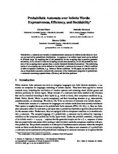
We now provide a few examples of probabilistic ω-automata to illustrate the defini¨ tion. For simplicity, we only give examples of probabilistic ω-automata with a Buchi acceptance condition. Given a PBA P with the acceptance condition F, intuitively, PrP (w) denotes the probability for the event “infinitely often F” under the scheduling policy induced by w. Recalling our LTL notations, this means that PrP (w) = PrP,w ("!F). In the pictures of PBA, we use boxes to denote the accepting states and circles for the non-accepting states. We might simply write a as label for a transition from p to q if δ( p, a, q) = 1. Label a, x with x ∈]0, 1[ for a transition from p to q denotes that δ( p, a, q) = x. An initial state will be indicated through an incoming edge, labeled with the initial probability of the state. Again, if the probability is 1, we might omit it. Example 3.4. Figure 1 shows a PBA P over the alphabet $ = {a, b} such that L>0 (P) = (a + b)∗ aω ,

L=1 (P) = b∗ aω ,

1

L> 5 (P) = b∗ ab∗ ab∗ aω

To see this, we first notice that only the words in (a + b)∗ aω have an accepting run, because the a-labeled self-loop in the accepting state p1 is the only outgoing transition of state p1 . On the other hand, Pr(aω ) = 1 (as the nonaccepting run p0 , p0 , p0 , . . . has probability 0 while all other runs for aω are accepting). Given a word σ = c1 c2 . . . c* baω Journal of the ACM, Vol. 59, No. 1, Article 1, Publication date: February 2012.

JACM5901-01

ACM-TRANSACTION

February 14, 2012

16:56

1:10

C. Baier et al.

b, 1; a, 12 1

a, 12

p0

a, 1 p1

Fig. 1. PBA P with L>0 (P) = (a + b)∗ aω .

P1 :

P2 : p0

b, c

b

q0

a, 12

a, 12

a, 12 p1

c

b

a, 12 p2

q1

q2

Fig. 2. PBA>0 for (ab + ac)∗ (ab)ω and for ∅.

# &k with ci ∈ {a, b}, the precise acceptance probability is therefore PrP (σ ) = 12 where k = |{i ∈ {1, . . . , *} : ci = a}|. Together, this yields L>0 (P) = (a + b)∗ aω , L=1 (P) = b∗ aω 1 and L> 5 (P) = b∗ ab∗ ab∗ aω .

Clearly, any DBA can be viewed as a PBA under any semantics, with δPBA ( p, a, q) = 1 if δDBA ( p, a) = {q} and µPBA (q0 ) = 1. On the other hand, it is well known that the 0 language (a + b)∗ aω cannot be recognized by a DBA, thus this example shows that PBA>0 are strictly more expressive than DBA. It is worth mentioning that the qualitative criteria “accepting runs have positive probability” is different from the acceptance criteria “there is an accepting run” in the context of languages of infinite words, while they agree for probabilistic automata viewed as acceptors for finite words. In fact, the na¨ıve transformation from PBA to NBA which relies on ignoring the probabilities, in general fails to yield an equivalent NBA. Example 3.5. Consider, for example, the automaton P1 on the left of Figure 2. Its underlying NBA (that we obtain by ignoring the probabilities) accepts the language ((ac)∗ ab)ω whereas P1 , under the probable semantics, accepts the language (ab + ac)∗ (ab)ω . The intuitive argument why any word w in (ab + ac)ω with infinitely many c’s is rejected relies on the observation that almost all runs2 for w are finite and end in state p1 (where the next input symbol is c and cannot be consumed in state p1 ). Under the almost-sure semantics, the language accepted by P1 is (ab)ω . Another example is the PBA P2 on the right of Figure 2. It accepts (under any semantics) the empty language as any infinite word in (ab + ac)ω has exactly one accepting run in P2 , but its probability is 0. However, the underlying NBA accepts the language (ab + ac)ω . 2 The formulation “almost all runs have property X ” means that the probability measure of the runs where property X does not hold is 0.

Journal of the ACM, Vol. 59, No. 1, Article 1, Publication date: February 2012.

JACM5901-01

ACM-TRANSACTION

February 14, 2012

16:56

Probabilistic ω-Automata

1:11

a, 1−λ 1

a, λ p0

a, 1 p1

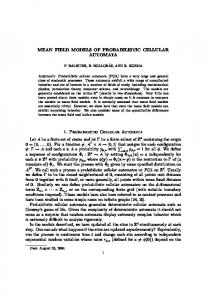
b, 1 Fig. 3. PBA>0 Pλ accepts a non-ω-regular language (where 0 < λ < 1).

4. A CLOSER LOOK ON PBA

In the last section, we introduced general probabilistic ω-automata, and presented a few simple examples of PBA. We now examine PBA a little closer. 4.1. PBA under the Probable Semantics

In this section, we report on results on the expressiveness and efficiency of PBA under the probable semantics. We also show that the precise transition probabilities matter for the accepted language of a PBA>0 and present a pumping lemma. 4.1.1. Expressiveness. First, we establish that the class of languages that can be accepted by a PBA>0 strictly contains the class of ω-regular languages.

THEOREM 4.1 (PBA>0 ARE STRICTLY MORE EXPRESSIVE THAN NBA). ω-reg ! L(PBA>0 ) The proof of Theorem 4.1 is split into two parts. In Lemma 4.2, we show that for any NBA A there exists a PBA P such that L>0 (P) = L(A). Then, in Lemma 4.3 we provide an example of a PBA>0 for which the accepted language is not ω-regular. LEMMA 4.2 (FROM NBA TO PBA>0 ). For any NBA A, there is a PBA P such that L (P) = L(A) and |P| = O(exp(|A|)). >0

PROOF. Following Courcoubetis and Yannakakis [1995], we call an NBA A deterministic in limit if |δ( p, a)| ≤ 1 for any state p that is reachable from an accepting state q ∈ F and any symbol a ∈ $. If we regard an NBA A that is deterministic in limit as a PBA P (with arbitrary probability distributions to resolve the nondeterministic choices) then L(A) = L>0 (P). Courcoubetis and Yannakakis [1995] provided a transformation from a given NBA A into an equivalent NBA that is deterministic in limit and whose size is (single) exponential in |A|. This yields the proof of the lemma. It remains to provide an example of a PBA>0 that recognizes a language that is not ω-regular. LEMMA 4.3 (A PBA>0 THAT ACCEPTS A NON-ω-REGULAR LANGUAGE). picted in Figure 3 accepts a language that is not ω-regular.

The PBA>0 de-

PROOF. For each real number λ ∈]0, 1[, the PBA>0 Pλ depicted in Figure 3 recognizes the language: ( ) ∞ " Lλ = ak1 bak2 bak3 b . . . | k1 , k2 , k3 . . . ∈ N≥1 s.t. (1 − (1 − λ)ki ) > 0 . i=1

Note that L (Pλ ) ⊆ (a b) as every accepting run for an infinite word w that has only finitely many b’s has to stay in state p0 from some point on. But such runs occur with probability 0. Let w = ak1 bak2 . . . ∈ (a+ b)ω . Starting in p0 and reading the first k1 letters a, the automaton reaches state p0 with probability (1 − λ)k1 and thus state p1 with >0

+

ω

Journal of the ACM, Vol. 59, No. 1, Article 1, Publication date: February 2012.

JACM5901-01

ACM-TRANSACTION

February 14, 2012

16:56

1:12

C. Baier et al.

probability 1 − (1 − λ)k1 . Reading the first b the automaton thus rejects with probability (1 − λ)k1 and carries on to read the input word with probability 1 − (1 − λ)k1 . This shows that the probability not to reject while reading the word w is ∞ " i=0

(1 − (1 − λ)ki )

and moreover this agrees with the probability to visit infinitely often the final state p0 . Therefore, L>0 (Pλ ) = Lλ . The following argument shows that L>0 (Pλ ) is not ω-regular. It is easily seen that L>0 (Pλ ) is nonempty and obviously it does not contain any lasso-shaped word, that is, a word of the form xyω , x ∈ $ ∗ and y ∈ $ + . As any nonempty ω-regular language contains a lasso-shaped word (since it can be described by an NBA with an accepting cycle), it follows that L>0 (Pλ ) is not ω-regular.

Remark 4.4 (Nonregular Convergence). The nonregular convergence condition for the words accepted by the PBA>0 Pλ in Figure 3 can be explained by the observation that there are finite input words that Pλ rejects with arbitrary small probability. More precisely, when Pλ tries to read a finite word akb in state p0 then Pλ fails to consume the last letter b (i.e., rejects) with probability (1 − λ)k. If k tends to infinity, the rejecting probability (1 − λ)k tends to 0. Similarly, there are PBA and infinite input words that have accepting runs in the underlying nondeterministic automaton, while the probabilities for the run fragments connecting two accepting states tend to zero. Such an example is described in Section 4.2.

We showed that PBA>0 are strictly more expressive than ω-regular languages. Note that Baier and Gr¨osser [2005] identified a subclass of PBA>0 that corresponds to the class of ω-regular languages. For this purpose, Baier and Gr¨osser [2005] introduced socalled uniform PBA>0 . The uniformity condition is semantic in nature and is motivated by the observation made in Remark 4.4 and serves to rule out PBA>0 with “non-regular converging behaviors”, as it is the case for the PBA>0 Pλ of Figure 3. Just recently, Chadha et al. [2009b] introduced syntactic restrictions on PBA that capture regularity, both for the probable as well as the almost-sure semantics. The restriction considered imposes a hierarchical structure on the PBA. 4.1.2. Efficiency. We saw in Lemma 4.2 that, for each NBA, there exists an equivalent PBA>0 of size exponential in the size of the NBA. We now study the efficiency of PBA>0 in more detail and show that for some languages, PBA>0 can be exponentially better than nondeterministic ω-automata.

LEMMA 4.5 (PBA>0 CAN BE EXPONENTIALLY SMALLER THAN NSA). There exists a family (Ln)n∈N of ω-regular languages in {a, b}ω such that for every n, Ln is accepted by a PBA n under the probable semantics with 2n states, while any NSA for Ln has at least 2n states. PROOF. The language Ln = {xyω : x ∈ {a, b}∗ , y ∈ {a, b}n} is accepted by the PBA>0 P shown in Figure 4. Note that all states of P are accepting and that all states except na have a b-transition to the state 1b and all states except nb have an a-transition to the state 1a . We assume uniform distributions: All edges except the a-edge in state na and the b-edge in state nb are taken with probability 12 . Let w = a1 a2 . . . ∈ / Ln. Then there are infinitely many indices i such that ai = a ∧ ai+n = b. Since every state except the state nb has an a-transition to state 1a , the stochastic process induced by P and the input word w will almost surely be infinitely often in state 1a with the letter b coming up in n steps. But each time (with probability Journal of the ACM, Vol. 59, No. 1, Article 1, Publication date: February 2012.

JACM5901-01

ACM-TRANSACTION

February 14, 2012

16:56

Probabilistic ω-Automata

1:13 a

a

a

a 1a

a, b

2a

3a

a, b

b

a, b

a, b

a, b

a, b

na

b

a

b a

a, b

1b

a

a, b

2b

b

nb

3b

b

b

b

Fig. 4. PBA>0 for Ln as in the proof of Lemma 4.5. 1

) the process will have moved to the state na while reading the upcoming n − 1 2n−1 letters, thus rejecting upon reading the b. Thus, almost surely the process will reject 1 infinitely often with probability 2n−1 which shows that almost all runs are rejecting. P >0 Thus, Pr (w) = 0 and w ∈ / L (P). Therefore, L>0 (P) ⊆ Ln. On the other hand, given a word w ∈ Ln, we can write w as xyω with x ∈ {a, b}∗ and y ∈ {a, b}n. Then, π = 1c1 , . . . , 1ck , 1d1 is a run for xd1 , where x = c1 c2 . . . ck and y = d1 d2 . . . dn. (The c’s and d’s are symbols in {a, b}.) The probability for this run is strictly greater than zero. Since from that state 1d1 on, the process will never reject while reading the remaining suffix of w and since every infinite run is accepting, this shows that w will be accepted with a probability greater than zero. This yields Ln ⊆ L>0 (P). n It remains to show that any NSA for Ln has at least 2n states. Let A be an NSA with L(A) = Ln. Let x = c1 . . . cn, y = d1 . . . dn ∈ {a, b}n such that c1 . . . cn (= di . . . dnd1 . . . di−1 for all i = 1, . . . , n.

(+)

Then any two accepting cycles for (c1 . . . cn) and (d1 . . . dn) are disjoint, or else A would accept some word of the form (a + b)∗ (c1 . . . c j di . . . dnd1 . . . di−1 c j+1 . . . cn)ω . But such a n word is not in Ln because of (+). Thus, A has at least 2n disjoint accepting cycles, which proves the claim. Another example illustrates the efficiency of PBA>0 compared to NBA: ω

ω

LEMMA 4.6 (PBA CAN BE EXPONENTIALLY SMALLER THAN NBA). Let Ln be the language consisting of all infinite words w = a1 a2 a3 . . . ∈ {a, b, c}ω such that for all 0 ≤ i < n: ∞

∞

∃ k such that akn+i = a if and only if ∃ k such that akn+i = b.

Then, Ln is accepted by a PBA #(2n) states.

>0

(++)

2

with O(n ) states, while any NBA that accepts Ln has

PROOF. Safra and Vardi [1989] proved that any NBA that accepts Ln has #(2n) states. But there exists an NSA that accepts Ln and consists of O(n) states. It remains to show that there is a PBA>0 of quadratic size that accepts Ln. For any word w = a1 a2 . . . ∈ Ln, we refer to the suffix arn+1 arn+2 . . . such that

(1) for all 0 ≤ i < n either akn+i = c for all k ≥ r or there are infinitely many k, * with akn+i = a and a*n+i = b and (2) r is minimal with respect to (1) Journal of the ACM, Vol. 59, No. 1, Article 1, Publication date: February 2012.

JACM5901-01

ACM-TRANSACTION

February 14, 2012

16:56

1:14

C. Baier et al.

a,b,c

2

a,b,c

a,b,c

0

a,b,c

a,c

0

1

a

b

b

c

accept(1,b)

a,c

1

2

a

b

b

c

2

4

2

accept(3,b)

3

a

n-1

a,c

a

0

with

2

3

a,b,c

a,b,c

4

a accept(3,a)

c

n-1

a,b,c

b

0

b,c

n-1

a,b,c

accept(0,a)

accept(0,b)

PBA>0

a,b,c

a,b,c

1

a

b

Fig. 5.

3

a,b,c

a,b,c

a,b,c

a,b,c

b

b,c

c

a,b,c

a,b,c

a,b,c

c

c

a,b,c

1 a

2 b

1

b,c

accept(2,a)

a,b,c

a,c

2

a,b,c

a,b,c

a,b,c

a,b,c

a,b,c

accept(2,b)

a,b,c

a,b,c

a

1

a,b,c

0

a,b,c

a,b,c

a,b,c

b,c

accept(1,a)

a,b,c

3

1

O(n2 )

a,b,c

states, while any equivalent NBA has #(2n) states.

as the legal suffix of w. A PBA>0 P with O(n2 ) states that accepts Ln is depicted in Figure 5 (we assume uniform distributions). All following calculations with indices i, j ∈ {0, 1, . . . , n − 1} are modulo n, that is, we simply write i + 1 instead of (i + 1) mod n. The automaton P consists of: —a subautomaton Pinit that serves to wait until the legal suffix of w starts. It consists of a cycle of accepting states 0, 1, . . . , n − 1 that are passed in this order. —subautomata P(i,a) and P(i,b) that are entered from Pinit when reading the letter a (respectively, b) in state i. The automata P(i,a) and P(i,b) consist of a cycle of nonaccepting states 0, 1, . . . , n − 1 that are passed in this order. They are entered in state i + 1 (coming from state i of Pinit upon reading the letter a (respectively b)) and can be left via an accepting state only when reading the letter b (respectively, a) in state i. Note that for all words w ∈ {a, b, c}ω all runs are infinite and almost all runs leave the subautomaton Pinit if w contains infinitely many a’s or b’s. The automaton rejects if it enters P(i,a) or P(i,b) , but there is no following position kn + i with akn+i = b or akn+i = a, respectively. Let w = a1 a2 . . . ∈ / Ln. Without loss of generality, there is some r ≥ 0 and some i ∈ {0, 1, . . . , n − 1} such that akn+i = a for infinitely many k, but akn+i (= b for all k ≥ r. Assume for simplicity that for all j (= i, condition (++) is fulfilled. We now consider the stochastic process induced by P and w. As there are infinitely many such k’s, the process will almost surely enter P(i,a) but never leave it. Hence, almost all runs for w are Journal of the ACM, Vol. 59, No. 1, Article 1, Publication date: February 2012.

JACM5901-01

ACM-TRANSACTION

February 14, 2012

16:56

Probabilistic ω-Automata

1:15

rejecting which yields w ∈ / L>0 (P). If (++) is violated for several indices i ∈ {0, . . . , n−1}, then the process will almost surely end up in several P(i,a) and P(i,b) and never leave those. Hence, almost all runs for w are rejecting which yields w ∈ / L>0 (P). Vice-versa, let w = a1 a2 . . . ∈ Ln and arn+1 , arn+2 , . . . be the legal suffix of w. Then, all runs for w that stay in Pinit for the first rn input symbols (the prefix a1 . . . arn of w) will infinitely often be in Pinit and are therefore accepting. Hence, PrP (w) > 0 and w ∈ L>0 (P).

These examples illustrate that PBA>0 can yield much more compact representations of ω-regular languages than nondeterministic automata. Vice-versa, Baier and Gr¨osser [2005] provides an example for a family of ω-regular languages with nondeterministic ¨ Buchi automata of linear size, while all uniform PBA>0 have at most #(2n) states. It is open whether the uniformity condition in the proof of Baier and Gr¨osser [2005] can be dropped. 4.1.3. The Precise Probabilities Matter under the Probable Semantics. We will show that the precise transition probabilities of a probabilistic automaton play a role for the language that is accepted under the probable semantics. The PBA Pλ , represented in Figure 3, page 11, illustrates this phenomenon.

THEOREM 4.7 (THE PRECISE PROBABILITIES MATTER FOR PBA>0 ). For any 0 < λ < µ < 1, L>0 (Pλ ) (= L>0 (Pµ ). * PROOF. Recall that L>0 (Pλ ) = {ak1 bak2 b . . . | i≥1 (1 − (1 − λ)ki ) > 0}. Assuming λ < µ, it is easy to see that L>0 (Pλ ) ⊆ L>0 (Pµ ) since 1 − (1 − µk) > 1 − (1 − λk) for any k ∈ N. To prove that the inclusion is strict, let us explain how to build a sequence (ki )i∈N such that " " (1 − (1 − λ)ki ) = 0and (1 − (1 − µ)ki ) > 0. i≥1

i≥1

This suffices to prove that L>0 (Pλ ) (= L>0 (Pµ ), since the infinite word ak1 bak2 b . . . will then be in L>0 (Pµ ) \ L>0 (Pλ ). n In order to build such a sequence, let n, m ∈ N such that 1 − µ < m < 1 − λ. We define the sequence (ki )i∈N as a nondecreasing sequence of natural numbers with 3( m )j4 n elements equal to j, where given a positive real number x, 3x4 denotes the integer part of x. Observe first that " + (1 − x ki ) is positive if and only if the series log(1 − x ki ) converges. i≥1

i≥1

!

Since log(1−ε) ∼ε6→0 −ε, the latter series behaves as i≥1 x kj (i.e., either both converge, or both diverge). For our chosen sequence (ki )i∈N , it holds that + + ,- m. j / · x j, x ki = n i≥1

j≥1

!

! which converges if and only if j≥1 3( m ) j 4 · x j + j≥1 (( m ) j − 3( m ) j 4) · x j converges. (Note n n n 1 that the second summand is less than 1−x ). Altogether, + - m. j " ki (1 − x ) is positive if and only if · x j converges, n i≥1

which is equivalent to

j≥1

m n

· x < 1, that is, x
0 ). Let P = (Q, $, δ, µ, F) be a PBA. Then, for each word ρ ∈ L>0 (P) and for all i ∈ N there exist finite words u, v, w ∈ $ ∗ and an infinite word x ∈ $ ω such that (1) ρ = uvwx, (2) |u| = i, |vw| ≤ |Q| and |w| ≥ 1, and (3) uvw * x ∈ L>0 (P) for all * ∈ N.

PROOF. Let n = |Q| be the number of states in P. Given ρ = a1 a2 a3 . . . ∈ L>0 (P) and i ∈ N we regard the finite prefix y = a1 a2 . . . ai . . . ai+n of ρ consisting of the first m = i + n letters of ρ. As PrP (ρ) is positive, there is a run a1

a2

ai

ai+1

am

σ = q0 − → q1 − → ... − → qi − → ... − → qm

for y in P such that the probability of all accepting runs for ρ in P that start with σ is positive. In particular, the probability for the accepting runs for the infinite suffix am+1 am+2 am+3 . . . of ρ that start in state qm is positive. We now pick word positions j and k such that i ≤ j < k ≤ m and q j = qk. Then, a1

ai

q0 − → ... − → qi aj ai+1 qi − → ... − → qj a j+1 ak q j −→ . . . − → qk ak+1 am qk −→ . . . − → qm

is a run for is a run for is a run for is a run for

u= v= w= z=

a1 . . . ai ai+1 . . . a j a j+1 . . . ak ak+1 . . . am

Furthermore, let x = zam+1 am+2 am+3 . . . = ak+1 ak+2 ak+3 . . .. Obviously, the first two conditions hold as we have (1) ρ = uvwx and (2) |u| = i and |vw| = k − i ≤ n. It remains to check the pumping condition (3). Let * ∈ N. As q j = qk the above runs for u, v, w and z can be composed to obtain a run for the finite word uvw* z that starts in q0 and ends in state qm. Since the probability for the accepting runs for the infinite suffix am+1 am+2 am+3 . . . of ρ that start in state qm is positive, we get PrP (uvw * x) > 0, and hence uvw* x ∈ L>0 (P). As for other types of automata, the pumping lemma can be useful to establish that a certain language is not PBA>0 -recognizable. We can show the following, where ω-CF denotes the class of ω-context free languages. COROLLARY 4.9. ω-CF (⊆ L(PBA>0 ).

PROOF. For instance, there is no PBA>0 that accepts the ω-context free language L = {anbn(a + b)ω |n ≥ 1}. Suppose by contradiction that such a PBA>0 P exists. Let n be the number of states in P. We now apply the pumping lemma to the word ρ = anbnaω ∈ L>0 (P) and the word position i = 0, which yields the existence of finite words v, w and an infinite word x such that ρ = vwx, w is nonempty and |vw| ≤ n and vw* x ∈ L>0 (P) for all * ≥ 0. Since |vw| ≤ n, both words v and w contain just a’s, say v = a j , w = ak where k ≥ 1 (as w is nonempty). Then x = an− j−kbnaω and vw 0 x = vx = an−kbnaω ∈ / L, which is a contradiction. 4.2. PBA under the Almost-Sure Semantics

In this section, we investigate the almost-sure semantics for PBA, that is, a PBA accepts a word if the set of accepting runs for this word has measure 1. We start our discussion Journal of the ACM, Vol. 59, No. 1, Article 1, Publication date: February 2012.

JACM5901-01

ACM-TRANSACTION

February 14, 2012

16:56

Probabilistic ω-Automata

1:17 a, 1−λ

p2

b, 1

a, 1

a, λ

p1

a, 1−λ

a, 1−λ

a, λ

a, λ

pF

b, 1

p0

0λ (0 < λ < 1) with L=1 (P 0λ ) non-ω-regular. Fig. 6. PBA P

with an example that has the interesting property that each word is either accepted with probability 0 or 1. 0λ shown in Figure 6. Under the almost-sure seman4.2.1. Example. Regard the PBA P tics it accepts the following language ( ) ∞ " 0 Lλ = ak1 bak2 bak3 b . . . | k1 , k2 , k3 . . . ∈ N≥1 such that (1 − (1 − λ)ki ) = 0 . i=1

0λ ) is indeed 0 We now check that L (P Lλ . Starting in p0 (or pF ), (1−λ)ki is the probability ki ki to be in p2 after reading the word a . Hence, 1−(1−λ)* represents the # & probability to be in state p1 after the input word aki . As a consequence i 1 − (1 − λ)ki is the probability to avoid forever the final state pF . The probability to visit pF after reading the word ak1 bak2 b . . . akN−1 b and to avoid pF from then on is therefore " (1 − λ)kN−1 · (1 − (1 − λ)ki ) =1

i≥N

with the convention k0 = 0. Hence, given an input word w = ak1 bak2 bak3 b . . ., the probability to avoid qF from some point on is   + "# & (1 − λ)kN−1 1 − (1 − λ)ki . N≥1

!

0λ P

i≥N

* kN−1

ki =1 0 0 Thus, Pr (w) = 1 − N≥1 ((1 − λ) i≥N (1 − (1 − λ) )). To prove that L (Pλ ) = Lλ , we need to show that   " + " 0 (1 − λ)kN−1 PrPλ (w) = 1 − (1 − (1 − λ)ki ) = 1 ⇐⇒ (1 − (1 − λ)ki ) = 0. N≥1

⇐ : Suppose that Hence,

i≥1 (1

− (1 − λ)ki ) = 0. Then,

+

N≥1 0λ P

i≥1

i≥N

*

This yields Pr (w) = 1.



(1 − λ)kN−1

"

i≥N

*

i≥N (1

− (1 − λ)ki ) = 0 for all N ∈ N. 

(1 − (1 − λ)ki ) = 0.

Journal of the ACM, Vol. 59, No. 1, Article 1, Publication date: February 2012.

JACM5901-01

ACM-TRANSACTION

February 14, 2012

16:56

1:18

C. Baier et al.

* ⇒ : Assume now that i≥1 (1 − (1 − λ)ki ) > 0. Then   + " " (1 − λ)kN−1 (1 − (1 − λ)ki ) > (1 − λ)k0 (1 − (1 − λ)ki ) > 0 N≥1

i≥1

i≥N

0λ P

and therefore Pr (w) < 1.

Remark 4.10. We are even able to prove that each word w ∈ {a, b}ω is either 0λ with probability 0 or with probability 1, that is, PrP0λ (w) ∈ {0, 1} for all accepted by P ω 0λ is quite remarkable as it has the property that w ∈ {a, b} . Thus, the automaton P 0λ ) = L>0 (P 0λ ). We call such an automaton a 0/1-automaton. L=1 (P * The following calculation shows the claim. Assume that i≥1 (1 − (1 − λ)ki ) > 0. The goal is to show that +

N≥1



(1 − λ)kN−1

"

i≥N



(1 − (1 − λ)ki ) = 1

.

ki

With θi = 1 − (1 − λ) , we obtain:     + " + " (1 − λ)kN−1 (1 − θ N−1 ) (1 − (1 − λ)ki ) = θi  N≥1

i≥N

N

= =



+



N



N

N→∞

N " i=1

θi ·

θi − θ N−1

"

"

i≥N

= lim

0 (= c =

"

i≥N



+

To conclude, we have to show that lim N→∞ *∞ c := i=1 θi > 0. But this is obvious since

i≥N

*

"

i≥N

i≥N θi

∞ "

θi − θi

"

i≥N

i≥N−1



θi 



θi 

since θ0 = 0. = 1, using the assumption

θi .

i=N+1

As the left factor converges to c if N tends to infinity, the right factor has to converge to 1 which shows the claim. 4.2.2. The Precise Probabilities Matter. The previous example shows that alike to the setting of PBA>0 , the precise transition probabilities also matter for PBA under the almost-sure semantics.

THEOREM 4.11 (THE PRECISE PROBABILITIES MATTER FOR PBA=1 ). For any 0 < λ < µ < 0λ ) (= L=1 (P 0µ ). 1, L=1 (P

0λ ) = (a+ b)ω \ PROOF. The theorem follows immediately from Theorem 4.7 since L=1 (P L (Pλ ). >0

Journal of the ACM, Vol. 59, No. 1, Article 1, Publication date: February 2012.

JACM5901-01

ACM-TRANSACTION

February 14, 2012

16:56

Probabilistic ω-Automata

1:19

4.2.3. Expressiveness of PBA under the Almost-Sure Semantics. We first give examples to ¨ show that the class of probabilistic Buchi automata under the almost-sure semantics ¨ is not closed under complementation. We then observe that for probabilistic Buchi automata, the switch from the probable semantics to the almost-sure semantics leads to a loss of expressiveness. At last we show that the class of languages definable by PBA=1 (respectively, its complement) is not comparable to the class of ω-regular languages.

LEMMA 4.12. L(PBA=1 ) is not closed under complementation. PROOF. It is evident that each DBA P can be viewed as a PBA and that LDBA (P) = L=1 (P). The language (a∗ b)ω can be recognized by a DBA and hence by a PBA=1 . However, its complement (a + b)∗ aω cannot be recognized by a PBA=1 . Suppose by contradiction that there is a PBA P = (Q, {a, b}, δ, µ0 , F) such that L=1 (P) = (a + b)∗ aω . Without loss of generality, we may assume that all states p ∈ Q are reachable from some initial state. Let ρ p ∈ {a, b}∗ be a finite word such that p ∈ δ(qinit , ρ p) where qinit is an initial state, that is, µ0 (qinit ) > 0. Since the word ρ paω belongs to (a + b)∗ aω , it holds that PrP (ρ paω ) = 1. But then the set of accepting runs for aω starting in p must have probability measure 1, that is, PrPp (aω ) = 1. Thus, there exists np ∈ N≥1 such that δ( p, anp ) ∩ F (= ∅. Let n = max np and w˜ = (anb)ω ∈ / (a + b)∗ aω . For p ∈ Q, let θ p be p∈Q

the probability to visit at least once an accepting state q ∈ F when scanning the word an from p. Note that θ p > 0 since np ≤ n and δ( p, anp ) ∩ F (= ∅. Let θ = min p∈Q θ p. Then, θ > 0 and for each k ≥ 0 and each state p ∈ δ(Qinit , (anb)k), the probability to enter F at least once while reading an from p is at least θ . But then almost all runs ˜ = 1, which contradicts the assumption for w˜ visit F infinitely often. That is, PrP (w) that L=1 (P) = (a + b)∗ aω . Hence, the class of languages L(PBA=1 ) is not closed under complementation. The next theorem shows that both the class of languages that are accepted by PBA under the almost-sure semantics as well as its complement are strictly included in the class of languages that are accepted by PBA under the probable semantics. THEOREM 4.13. (a) L(PBA=1 ) ! L(PBA>0 ) and (b) L(PBA=1 ) ! L(PBA>0 ). PROOF. (a) Let P = (Q, $, δ, µ0 , F) be a PBA and L = L=1 (P) the language of P under the almost-sure semantics. We will transform P into an equivalent 0/1-PBA P / , that is a PBA that accepts each word either with probability 0 or 1. The idea to define P / is to pick at random some word position i where P could be in a state p ∈ Q \ F and to check whether from this position i on, the probability in P for the event "¬F is positive. If so, then the input word is rejected by P with positive probability, and therefore, it does not belong to L. Formally, we define the PBA P / as (Q / , $ / , δ / , µ/0 , F / ) where Q / = 2 Q ∪ Q × 2 Q,

F / = 2Q

and µ/0 (Qinit ) = 1 where Qinit = {q ∈ Q : µ0 (q) > 0}. The transition probabilities in P / are defined as follows. If R ⊆ Q and a ∈ $ then δ / (R, a, S) = 1 if S = δ(R, a) ⊆ F. For S = δ(R, a) and S \ F (= ∅ we define δ / (R, a, S) = 12 , δ / (R, a, ( p, S)) =

1 2·|S\F|

for all p ∈ S \ F.

For p ∈ R\ F, q ∈ Q and S = δ(R, a) we set δ / (( p, R), a, (q, S)) = δ( p, a, q). For p ∈ R∩ F and S = δ(R, a) we set δ / (( p, R), a, S) = 1. In all remaining cases, we set δ / (·) = 0. Journal of the ACM, Vol. 59, No. 1, Article 1, Publication date: February 2012.

JACM5901-01

ACM-TRANSACTION

February 14, 2012

16:56

1:20

C. Baier et al.

i Now assume w ∈ L=1 (P), thus PrP,w ("!F) = 1. This implies PrP,w↑ ("!F) = 1 for t i−1 all i ∈ N≥1 and all states t ∈ δ(s, w↑ ), where µ0 (s) > 0. Thus, whenever P / enters its Q × 2 Q part while reading w, it will afterwards reach a state ( p, R) where p is an accepting state of P with probability one. As from such states δ / (.) leads to an / accepting state of P / with probability 1 (in one step), this shows that PrP ,w ("!F / ) = 1, >0 / so w ∈ L (P ). Assume w ∈ / L=1 (P), thus PrP,w (!"¬F) > 0. Then, there exists an i ∈ N≥1 such that P,w =i Pr (! "¬F) > 0, where !=i "¬F denotes the event that after the (i − 1)st step only states of ¬F will be visited. Obviously

(i) PrP,w (!= j "¬F) ≥ PrP,w (!=i "¬F) > 0 for all j > i. Let θ := PrP,w (!=i "¬F). As θ > 0, it holds that

(ii) for all j > i and all runs q0/ , q1/ , q2/ , . . . of w in P / : q/j | 2 Q ∩ ¬F (= ∅, where q/j | 2 Q = R j if q/j = R j is a state in the 2 Q part of P / and q/j | 2 Q = R j if q/j = (r j , R j ) is a state in the Q × 2 Q part of P / . Note that for the second statement (ii) the existence of a single run of w in P satisfying !=i "¬F suffices as the automaton P / performs a standard powerset construction on the 2 Q component in all its states. Examining the construction of P / shows that after reading the first i letters of w, whenever P / is in its accepting 2 Q part, it will move with probability 12 to its nonaccepting Q × 2 Q part (because of (ii)) where it will stay forever with probability at least θ (because of (i) and the fact that the nonaccepting Q × 2 Q part can only be left via a state (r, R) where r ∈ F). But this means that after the ith step (after reading w↑i ), the automaton P / will almost surely reach its nonaccepting part and stay there forever which shows / PrP ,w ("!F / ) = 0, thus w ∈ / L>0 (P / ). This shows that L>0 (P / ) = L=1 (P). The strictness of the inclusion L(PBA=1 ) ! L(PBA>0 ) immediately follows from / L(PBA=1 ) (see proof of Lemma 4.12). ω-reg ⊆ L(PBA>0 ) and the fact that (a + b)∗ aω ∈ (b) Given a PBA P = (Q, $, δ, µ0 , F) we can trivially construct a PBA P / = (Q / , $, δ / , µ/0 , F / ) of the same size such that L>0 (P / ) = $ ω \ L=1 (P). We define P / as indicated in the following picture (see Gr¨oßer [2008]).

{

F!

P! P

∈F

s!

a, p

∈F

P

Σ,1 qrej

a,

a, p2

s!

1 2

Q / = Q∪ {qrej }. For q2 ∈ Q, we set δ / (q1 , a, q2 ) = δ(q1 , a, q2 ) if q1 ∈ Q\ F and δ / (q1 , a, q2 ) = 1 · δ(q1 , a, q2 ) if q1 ∈ F. For q1 ∈ F we set δ / (q1 , a, qrej ) = 12 . Moreover δ / (qrej , a, qrej ) = 1 2 for all a ∈ $, µ/0 (q) = µ0 (q) for q ∈ Q (thus µ/0 (qrej ) = 0) and F / = Q. Now assume w ∈ L=1 (P), hence PrP,w ("!F) = 1. Thus, reading w, the automaton P / will almost surely reach the non-accepting state qrej and will then loop in qrej forever. / / L>0 (P / ). So PrP ,w ("!F / ) = 0 and w ∈ =1 Assume w ∈ / L (P), thus PrP,w (!"¬F) > 0. Then there exists an i ∈ N≥1 such that P,w =i Pr (! "¬F) > 0, where !=i "¬F denotes the event that after the (i − 1)st step Journal of the ACM, Vol. 59, No. 1, Article 1, Publication date: February 2012.

JACM5901-01

ACM-TRANSACTION

February 14, 2012

16:56

Probabilistic ω-Automata

1:21 /

/

/

only states of ¬F will be visited. But PrP ,w ("!F / ) = PrP ,w ("F / ) ≥ PrP ,w (!=i "F / ) ≥ i ( 12 ) · PrP,w (!=i "¬F) > 0, so w ∈ L>0 (P / ). This shows that L>0 (P / ) = $ ω \ L=1 (P).

The strictness of the inclusion L(PBA=1 ) ! L(PBA>0 ) immediately follows from ω-reg ⊆ L(PBA>0 ) and the fact that (a∗ b)ω ∈ / L(PBA=1 ) as $ ω \ (a∗ b)ω = (a + b)∗ aω ∈ / =1 L(PBA ) (see proof of Lemma 4.12). Note that the inclusion (b) also follows from (a) and the fact that PBA>0 are closed under complementation (as proven later in Section 6). However, the construction in the proof of (a) as well as the complementation yield each an exponential blow-up.

It remains to show that the class of PBA=1 -recognizable languages and its complement are not comparable to the class of ω-regular languages. THEOREM 4.14. (a) ω-reg " L(PBA=1 ), (b) L(PBA=1 ) " ω-reg, (c) ω-reg " L(PBA=1 ) and (d) L(PBA=1 ) " ω-reg. PROOF. / L(PBA=1 ) (see (a) The claim immediately follows from the fact that (a + b)∗ aω ∈ proof of Lemma 4.12). 0λ from Figure 6, page 17. It holds that L=1 (P 0λ ) = (b) Consider the example PBA=1 P + ω >0 0λ ) ∪ (a b) \ L (Pλ ), where Pλ is represented in Figure 3, page 11. Hence, L=1 (P (a+b)∗ aω ∪b(a+b)ω ∪(a+b)∗ bb(a+b)ω is the complement of L>0 (Pλ ). As L>0 (Pλ ) is 0λ ) is a non-ω-regular language. not ω-regular, this immediately yields that L=1 (P (c)-(d) The claims follow from (b) (respectively, (a)) and the fact that ω-regular languages are closed under complementation. 4.3. PBA under the Threshold Semantics

In this section, we focus on the expressiveness of PBA under the threshold semantics. First, we will show that the exact threshold is of no importance for the class of accepted languages. 4.3.1. Comparison for Different Threshold Values

LEMMA 4.15. For all λ, µ ∈]0, 1[, L(PBA>λ ) = L(PBA>µ ).

PROOF. Let λ (= µ be two real numbers in ]0, 1[. From a given PBA P, we construct another PBA P / with L>λ (P) = L>µ (P / ). The construction depends on whether λ < µ or λ > µ. Assume first λ > µ. P / consists of a copy of P equipped with an extra rejecting sink state qrej . In P / , accepting states are exactly those of P, and the initial distribution µ/0 is defined by µ/0 ( p) = µλ µ0 ( p) for states from P and µ/0 (qrej ) = 1 − µλ . Given a word w, it / holds that PrP (w) = µλ PrP (w) and thus L>µ (P / ) = L>λ (P). Assume now λ < µ. Automaton P / consists of a copy of P with an extra accepting sink state qacc . The accepting states in P / are those of P together with qacc , and the initial probability distribution is defined by µ/0 ( p) = 1−µ µ ( p) for states in P and 1−λ 0 µ−λ P/ µ/0 (qacc ) = µ−λ . Given a word w, it holds that Pr (w) = + 1−µ PrP (w) and thus 1−λ 1−λ 1−λ L>µ (P / ) = L>λ (P). Journal of the ACM, Vol. 59, No. 1, Article 1, Publication date: February 2012.

JACM5901-01

ACM-TRANSACTION

February 14, 2012

16:56

1:22

C. Baier et al.

4.3.2. Comparison with Other Semantics. Let us now compare threshold PBA to PBA under other semantics. The class of languages accepted by PBA under the threshold semantics subsumes the class of languages accepted by PBA under the probable or the almost-sure semantics.

LEMMA 4.16. For every λ ∈]0, 1[, L(PBA>0 ) ⊆ L(PBA>λ ).

PROOF. Let P be a PBA, and λ ∈]0, 1[. The automaton P can be transformed into P / such that L>0 (P) = L>λ (P / ). The new PBA P / consists of a copy of P with an extra accepting sink state qacc . Accepting states of P / are those of P together with qacc , and the initial distribution µ/0 is defined by: µ/0 ( p) = (1 − λ)µ0 ( p) for states of P, and µ/0 (qacc ) = λ.

The latter lemma raises the question whether PBA with the probable semantics are as expressive as PBA with the threshold semantics. The following theorem shows that this is not the case. THEOREM 4.17 (THERE EXIST THRESHOLD-LANGUAGES NOT IN L(PBA>0 )). numbers λ ∈]0, 1[, it holds that L(PBA>λ ) (⊆ L(PBA>0 ).

For all real

PROOF. Note that, because of Lemma 4.15 it is sufficient to show the existence of a PBA P and a threshold λ ∈]0, 1[ such that L>λ (P) ∈ / L(PBA>0 ). The proof is based on an adaption of arguments provided by Paz [1971] for probabilistic finite automata (PFA). We identify any real number λ ∈]0, 1[ with the infinite word a1 a2 a3 . . . ∈ {0, 1}ω obtained by its binary representation λ=

∞ + i=1

ai 2−i = 0.a1 a2 a3 . . .

(where we assume that ai (= 0 for infinitely many indices i). We now consider the following languages Kλ ⊆ {0, 1}∗ : ( ) n + −i bi 2 > λ Kλ = b1 . . . bn | b1 , . . . , bn ∈ {0, 1} such that i=1

Paz [1971] has shown that Kλ is regular if and only if λ is rational. Rabin [1963] provided a PFA R such that for all finite words ρ ∈ {0, 1}∗ , PrR (ρ) > λ if and only if ρ ∈ Kλ . We modify this PFA R to a PBA P over the alphabet $ = {0, 1, c} that under the threshold semantics accepts the language Lλ = Kλ cω = {ρcω | ρ ∈ Kλ }.

when dealing with the threshold λ. For this, we add a new accepting state qacc with a c-self-loop and no other transitions (i.e., we set δP (qacc , c, qacc ) = 1 and δP (qacc , b, ·) = 0 for b ∈ {0, 1}) and c-transitions from each final state p in R to qacc (i.e., we set δP ( p, c, qacc ) = 1 for all final states p of R). The remaining transitions are as in R. Finally the acceptance set of P is defined as F = {qacc } and the initial distribution of P is the same as in R. It then holds for all words ρ ∈ {0, 1}∗ that PrP (ρcω ) = PrR (ρ). Furthermore, PrP (w) = 0 if w contains infinitely many 0’s or 1’s. Thus: L>λ (P) = {ρcω | PrR (ρ) > λ} = Kλ cω = Lλ .

Now fix an arbitrary irrational number λ ∈]0, 1[. Thus, by Paz [1971], Kλ is nonregular. It remains to show that there is no PBA P / such that L>0 (P / ) = Lλ . The intuitive argument will be the following. Suppose by contradiction that P / is a PBA with Journal of the ACM, Vol. 59, No. 1, Article 1, Publication date: February 2012.

JACM5901-01

ACM-TRANSACTION

February 14, 2012

16:56

Probabilistic ω-Automata

1:23

L>0 (P / ) = Lλ ⊆ {0, 1}∗ cω . Thus, each word that will be accepted with a positive probability has a suffix consisting only of c’s. But then, there is some “kind of underlying (finite word) automaton” in P / , that decides which of the prefixes “to accept”. Although this is a probabilistic automaton, as the acceptance threshold in P / is 0, this “underlying (finite word) automaton” will accept a regular language, which will contradict the assumption that λ is irrational. More formally, we first observe that whenever (T , A) is an accepting end component / of P / with PrP ,w ((T , A)) > 0 for some word w ∈ $ ω then A( p) = {c} for all states p ∈ T . (Otherwise, P / would accept some words that do not have a suffix consisting of c’s.) Let T0 be the set of states p in P / such that p ∈ T for some accepting end component (T , A) / of P / with PrP ,w ((T , A)) > 0 for some word w ∈ $ ω . Furthermore, let T0+ be the set of all states q in P / such that p ∈ δP / (q, cn) for some n ≥ 0 and p ∈ T0 . That is T0+ consists of all states from which a relevant accepting end component can be reached via a finite / ρ → q) > 0 for some initial state sequence of c’s. Whenever ρ ∈ {0, 1}∗ such that PrP (q0 − q0 and some state q ∈ T0+ , then /

/

ρ

/

cn

PrP (ρcω ) ≥ PrP (q0 − → q) · PrqP (q − → p) > 0 for some n ∈ N≥0 , some state q ∈ T0+ and some state p ∈ δP / (q, cn), where p is in a relevant accepting end component. This yields ρcω ∈ L>0 (P / ) = Lλ = Kλ cω ,

and therefore ρ ∈ Kλ . Vice-versa, if ρ ∈ Kλ , then ρcω ∈ Lλ = L>0 (P / ). Hence, there exists a state q ∈ T0+ such that q ∈ δP / (q0 , ρ) for some initial state q0 . This shows that Kλ agrees with the set of finite words ρ ∈ {0, 1}∗ such that δP / (q0 , ρ) ∩ T0+ (= ∅. But then, Kλ agrees with the language of the NFA resulting from P / by discarding all c-transitions, interpreting the probabilistic branches by nondeterministic choices and declaring the states in T0+ to be final. Thus, Kλ is regular. This contradicts the assumption that λ is irrational in which case Kλ is not regular, as shown by Paz [1971]. Remark 4.18 (Irrational Coefficients). Note that the PFA R used in the proof of Theorem 4.17 only contains rational transition probabilities as well as rational initial probabilities. So the constructed PBA P also only contains rational transition probabilities as well as rational initial probabilities. It is only the irrational threshold λ that makes the language L>λ (P) not PBA>0 -recognizable. In the transformations provided in this section (i.e., from a PBA>0 to a PBA>λ or from a PBA>λ to a PBA>µ ), it is important to notice that the transition probabilities are not changed. Only the initial probabilities are changed and as soon as λ is irrational, the resulting automaton might contain irrational initial probabilities (even if the original automaton did not). Also we can detail the relationships between L(PBA>0 ) and languages defined by PBA with rational or irrational thresholds. First, on the one hand there are only countably many languages defined by PBA under the threshold semantics and with rational thresholds, whereas as a consequence of Theorem 4.17 there are uncountably many languages defined by PBA under the threshold semantics with irrational thresholds. As a consequence, irrational thresholds do enhance the expressive power of PBA under the threshold semantics. Second, the class L(PBA>0 ) is closed under complementation, as we shall prove in Section 6.2, whereas it was shown in Chadha et al. [2011] that languages defined by PBA under the threshold semantics with rational thresholds are not. Hence, L(PBA>0 ) ! L(PBA>λ ) for irrational values of λ. Journal of the ACM, Vol. 59, No. 1, Article 1, Publication date: February 2012.

JACM5901-01

ACM-TRANSACTION

February 14, 2012

16:56

1:24

C. Baier et al.

5. PRA AND PSA

After the investigation of properties of PBA in the latter section, we now study other ¨ acceptance criteria than the Buchi condition for probabilistic automata as acceptors for infinite words. We concentrate here on Streett and Rabin acceptance since they will play a central role for our complementation operator. For each semantics, any PBA can be trivially seen as a PSA or PRA by replacing ¨ the Buchi acceptance set F with the singleton Streett (respectively, Rabin) acceptance set Acc = {(F, Q)} (respectively, {(∅, F)}). We explore here transformations from PRA>0 and PSA>0 to PBA>0 , and compare the expressiveness of probable and almost-sure semantics for PRA and PSA. In the following, in order to stress the acceptance condition of a given probabilistic ω-automaton P, we often index Pr and L with Rabin, Streett, or ¨ Buchi, and write, for example, PrPStreett or L>0 (P). Rabin 5.1. From GPBA>0 , PSA>0 and PRA>0 to PBA>0

We show that the transformations known for nondeterministic automata can easily be adapted to the probabilistic setting. Moreover, even more efficient transformations can be provided as we will see in the case of Streett acceptance. THEOREM 5.1 (FROM GPBA>0 , PRA>0

AND

PSA>0

TO

PBA>0 ).

(a) For any generalized probabilistic Buchi ¨ automaton P, there exists a PBA P / with >0 >0 / =1 =1 / L (P) = L (P ), L (P) = L (P ), and |P / | = O(m|P|) where m is the number of acceptance sets in P . (b) For any PRA P R, there exists a PBA P with L>0 (P R) = L>0 (P) and |P| = O(m|P R|). Rabin (c) For any PSA P S , there exists a PBA P with L>0 (P S ) = L>0 (P) and |P| = Streett O(m2m|P S |).

¨ PROOF. (a) In generalized Buchi automata, the acceptance condition consists of a set F = {F1 , . . . , Fn} where the Fi ’s are subsets of the state space Q. Acceptance of a run requires that each of the Fi ’s is visited infinitely often. In the nondeterministic case, it ¨ ¨ is well known that the Buchi and generalized Buchi acceptance conditions have equal power, in the sense that any generalized NBA G can be transformed into an equivalent NBA A. The idea behind this transformation is to work with n copies G1 , . . . , Gn of G where the outgoing transitions from an Fi -state in the ith copy are redirected to the (i + 1)th copy (modulo n), while outgoing transitions from other states stay in the same ¨ copy. The Buchi acceptance condition in the so-built NBA A consists of the F1 -states in G1 . The exact same technique yields a polynomial transformation from GPBA>0 to PBA>0 , and from GPBA=1 to PBA=1 . (b) Let P R = (QR, δ R, µ R, {(H1 , K1 ), . . . , (Hn, Kn)}) be a PRA. Then, we define the PBA P by extending P R by copies of the subautomata for the states not in Hi . From any (Ki \ Hi )-state in the main automaton, we have a probabilistic choice to stay in the main automaton or to move to the (QR \ Hi )-copy in which we try to visit infinitely often a Ki -state and which can only 5 be left to a rejecting sink state. Formally, P = (Q, δ, µ, F), where Q = {qrej } ∪ QR ∪ 1≤i≤n((QR \ Hi ) × {i}), µ = µ R and F = ∪1≤i≤n(Ki × {i}). The transition relation δ of P is chosen in such a way that for a ∈ $: δ( p, a, q) > 0 δ( p, a, 9q, i:) > 0 δ(9 p, i:, a, 9q, i:) δ(9 p, i:, a, qrej ) δ(qrej , a, qrej )

iff iff = = =

δ R( p, a, q) > 0 δ R( p, a, q) > 0 and p ∈ Ki \ Hi δ R( p, a, q) $q∈Hi δ R( p, a, q) 1.

(P R). It is straightforward to show that L>0 (P) = L>0 Rabin Journal of the ACM, Vol. 59, No. 1, Article 1, Publication date: February 2012.

JACM5901-01

ACM-TRANSACTION

February 14, 2012

16:56

Probabilistic ω-Automata

1:25

(c) Let P S = (QS , δ S , µ S , {(H1 , K1 ), . . . ,6 (Hn, Kn)}) be a PSA. We first observe n that the Streett acceptance condition i=1 ("!Hi ∨ !"¬Ki ) is equivalent to #6 & 6 7 I⊆{1,...,n} i∈I "!Hi ∧ i ∈I / !"¬Ki . We define the PBA P by extending P S by subautomata P I for any subset I of {1, . . . , n}. In each state of the main automaton we decide randomly to stay in the main automaton or to move to one of the subautomata P I . Once P I has been entered, it can only rejecting sink state. Intuitively, 6 6 be left to a 6 P I realizes the condition i∈I "!Hi ∧ i∈I / Ki ). Note / !"¬Ki ≡ i∈I "!Hi ∧ !"¬(∪i ∈I that such a condition is similar to a single Rabin condition except that it enforces a ¨ generalized Buchi condition on the Hi ’s, where i ∈ I. Thus the construction of the P I ’s is a combination of 5 the constructions used in (a) and (b). P I consists of copies of P S without the states in i∈I The / Ki . Formally, 5 the PBA P = (Q, δ, µ, F) is defined as follows. n state space is Q = {qrej } ∪ QS ∪ I⊆{1,...,n} QI where Q∅ = {9q, ∅: : q ∈ QS \ (∪i=1 Ki )} and $ % QI = 9q, I, i: : i ∈ I, q ∈ QS \ (∪i∈I / Ki ) for ∅ (= I ⊆ {1, . . . , n}. The initial distribution is µ = µ S . For states p, q ∈ QS with δ S ( p, a, q) > 0, we let: —δ( p, a, q) > 0, —δ( p, a, 9q, ∅:) > 0 and —δ( p, a, 9q, I, first(I):) > 0 for any nonempty subset I of {1, . . . , n}, assuming a fixed enumeration i0 , . . . , ik−1 of the elements in I and putting first(I) = i0 .

The transitions inside QI are defined in a similar way as in the transformation from GPBA to PBA: δ(9 p, I, i* :, a, 9q, I, ir :) = δ S ( p, a, q) if either (r = *) ∧ ( p ∈ / H* ) or δ S ( p, a, q) (r = (* + 1) mod |I|) ∧ ( p ∈ H* ) δ(9 p, I, i* :, a, qrej ) = $q∈∪i∈I/ Ki δ S ( p, a, q) δ(9 p, ∅:, a, 9q, ∅:) = δ S ( p, a, q) n δ(9 p, ∅:, a, qrej ) = $q∈∪i=1 Ki δ S ( p, a, q) δ(qrej , a, qrej ) = 1. % 5 $ ¨ The Buchi acceptance set in P is F = Q∅ ∪ I 9 p, I, first(I): ∈ QI : p ∈ Hfirst(I) where I ranges over all nonempty subsets of {1, . . . , n}. This construction ensures L>0 (P) = L>0 (P S ). Streett

As for nondeterministic automata, the transformation of a PSA>0 into an equivalent PBA>0 is more complicated than for Rabin automata and can cause an exponential blowup. However, we show here that a polynomial transformation can be provided. This stands in contrast to the nondeterministic case where it is known that there exist NSA of polynomial size, for which any equivalent NBA has exponentially many states [Safra and Vardi 1989]. THEOREM 5.2 (POLYNOMIAL TRANSFORMATION FROM PSA>0 TO PBA>0 ). For any PSA P S , there exists a PBA P with L>0 (P S ) = L>0 (P) and |P| = O(n2 |P S |), where n is the Streett number of acceptance pairs in P S .

PROOF. Let P S = (QS , $, δ S , µ0S , {(H1 , K1 ), . . . , (Hn, Kn)}) be a PSA. For simplicity, we may assume that Hi ∩ Ki = ∅ as otherwise Ki could be replaced with Ki \ Hi . Intuitively, the PBA P arises from P S by making several copies of P S : a subautomaton Pinit in which the process starts, a subautomaton Paccept which has to be visited infinitely often and which is reachable with positive probability via any outgoing transition from the states in Pinit , and subautomata Pi and Pi, j for i, j ∈ {1, . . . , n}, i (= j, that are reached from Paccept whenever a state in Ki is visited in Paccept . Subautomaton Pi can only be left via transitions from a Hi -state in Pi from which we move back to Paccept . Subautomaton Pi, j behaves as Pi , but in addition it takes into account the Streett-acceptance pair Journal of the ACM, Vol. 59, No. 1, Article 1, Publication date: February 2012.

JACM5901-01

ACM-TRANSACTION

February 14, 2012

16:56

1:26

C. Baier et al.

Fig. 7. Transition probabilities of the PBA constructed in the proof of Theorem 5.2 (where i, j, k ∈ {1, . . . , n} s.th. i (= j and j (= k (but possibly i = k)).

(H j , K j ). When a K j -state in Pi, j is reached, we randomly choose to stay in Pi, j or to move to P j or one of the subautomata P j,k. Formally, the PBA P = (Q, $, δ, µ0 , F) is defined as follows. The state space is 8 8 Q = Qinit ∪ Qaccept ∪ Qi ∪ Qi, j 1≤i≤n

1≤i, j≤n

i(= j

where Q∗ = {9q, ∗: : q ∈ QS }. The set of accepting states is F = Qaccept . The initial distribution is given by µ0 (9q, init:) = µ0S (q) and µ0 (9q, ∗:) = 0 for all other states 9q, ∗: ∈ Q. The transition probabilities in P are shown in Figure 7 where q, p ∈ QS . Here, i, j, k range over all indices in {1, . . . , m} with i (= j and j (= k (but possibly i = k). In the sequel, we refer to the fragment of the Q∗ -states as the P∗ -subautomaton. To explain the role of subautomata Pi, j and Pi , let us assume for simplicity that the acceptance condition consists of two pairs {(H1 , K1 ), (H2 , K2 )} such that K1 \ K2 (= ∅. Pi, j subautomata avoid to accept paths visiting infinitely many K2 states in P1 , without taking care of visiting infinitely many H2 states as well. Let k1 ∈ K1 \ K2 , k2 ∈ K2 , h1 ∈ H1 . Without loss of generality, assume k2 ∈ / H1 . Then, the nonaccepting (possible) path k1 , k2 , h1 , k1 , k2 , h1 , . . .

in the Streett automaton would be lifted with positive probability to accepting paths of the form . . . , 9k1 , accept:, 9k2 , 1:, 9h1 , 1:, 9k1 , accept:, 9k2 , 1:, 9h1 , 1:, . . .

¨ in the Buchi automaton. This kind of behavior is avoided thanks to the Pi, j subautomata. However, Pi subautomata need to be added as well. Indeed, without the Pi Journal of the ACM, Vol. 59, No. 1, Article 1, Publication date: February 2012.

JACM5901-01

ACM-TRANSACTION

February 14, 2012

16:56

Probabilistic ω-Automata

1:27

¨ subautomata, the Buchi automata could visit infinitely many K1 states while being in Paccept moving to P1,2 . If the automaton also visits infinitely many K2 states but no H1 ¨ states, the Buchi automaton will almost surely leave P1,2 and move to P2,1 which it can leave to Paccept if it visits infinitely many H2 states. Thus, it could accept although it might not satisfy the Streett condition {(H1 , K1 )}. This is shown in the following example. Assume the previous construction without the Pi subautomata. Assume that K1 \ K2 (= ∅, K2 \ H1 (= ∅ and H2 \ K1 (= ∅ and let k1 ∈ K1 \ K2 , k2 ∈ K2 \ H1 , h2 ∈ H2 \ K1 . Then, the nonaccepting (possible) path k1 , k2 , h2 , k1 , k2 , h2 , . . . in the Streett automaton would be lifted with positive probability to accepting paths of the form . . . , 9k1 , accept:, 9k2 , 1, 2:, 9h2 , 2, 1:, 9k1 , accept:, 9k2 , 1, 2:, 9h2 , 2, 1:, . . .

¨ in the Buchi automaton. To avoid this, we need the 6 Pi subautomata. S In the following, we will denote by AccPStreett = 1≤ j≤n("!K j ⇒ "!H j ) the Streett 7 S acceptance condition of P S and by AccPRabin = 1≤ j≤n(!"¬H j ∧ "!K j ) the acceptance condition obtained from the acceptance pairs in P S by interpreting them as a Rabin acceptance condition. We now show that L>0 (P) = L>0 (P S ). Buchi ¨ Streett S S (P S ), thus PrPS ,w (AccPStreett ) = 0 and7hence PrPS ,w (AccPRabin ) = 1. Consider ⊆: Let w ∈ / L>0 Streett a run π of P S that satisfies the Rabin condition 1≤ j≤n(!"¬H j ∧ "!K j ), thus there exists an index j such that π |= !"¬H j ∧ "!K j . Consider the liftings of π in the ¨ constructed Buchi automaton P. (By a lifting of π , we mean any run in P for w whose projection to the QS -components agrees with π .) As the above construction ensures that whenever a K j -state is visited in Paccept or Pi, j for some i (= j, then with equal positive probability one of the subautomaton P j or P j,k is entered. Hence, if infinitely often a K j -state is visited and the process does not stay forever in one of the subautomata Pi (for some i (= j) or Pk,* (where it cannot accept), then almost surely P j is entered. But P j can only be left via a H j -state. As π |= !"¬H j this ensures that almost all liftings of π will eventually stay in one of the subautomata Pi or Pi,k, S hence they will almost surely not be accepting. This shows that PrPS ,w (AccPRabin )=1⇒ P >0 >0 PrBuchi (w) = 0 and w ∈ / L (P ) ⇒ w ∈ / L (P). S ¨ Streett ¨ 6 Buchi ⊇: Let w ∈ L>0 (P S ), thus PrPS ,w ( 1≤ j≤n("!K j ⇒ "!H j )) > 0. As {π | π |= Streett 6 ! 6 6 PS 1≤i≤n("!Ki ⇒ "!Hi )} = J⊆{1,...,n} {π | π |= AccStreett ∧ j∈J "!K j ∧ j ∈J / !"¬K j }, there exists J ⊆ {1, . . . , n} such that   9 9 s ∧ "!K j ∧ !"¬K j  > 0. PrPS ,w AccPStreett

j∈J

j ∈J /

Since !"¬K j is the disjoint union of (!=*−1 K j ∧ "≥* ¬K j ), for * ∈ N, and since {j | j ∈ / J} is finite, there exists r ∈ N≥0 such that   9 9 P S ,w  Ps "!K j ∧ ">r ¬K j  > 0. AccStreett ∧ Pr j∈J

6

j ∈J /

6 >r s Let π S be a run in P S with π S |= AccPStreett ∧ j∈J "!K j ∧ j ∈J / " ¬K j . Then almost all liftings of π S to runs for w in P that stay in Pinit for the first r input symbols and

Journal of the ACM, Vol. 59, No. 1, Article 1, Publication date: February 2012.

JACM5901-01

ACM-TRANSACTION

February 14, 2012

16:56

1:28

C. Baier et al.

eventually enter Paccept are accepting. This yields   9 9 1 P P S ,w  Ps PrBuchi (w) ≥ r+1 · Pr "!K j ∧ ">r ¬K j  > 0 AccStreett ∧ ¨ 2 j∈J

j ∈J /

and w ∈ LBuchi (P). ¨ >0

5.2. From PBA>0 to 0/1-PRA

In this section, we will describe how a given PBA>0 P can be transformed into an equivalent 0/1-PRA P R, that is a PRA such that every infinite word is either accepted with probability 0 or 1. This result will play a crucial role in Section 5.3 and for the complementation of PBA under the probable semantics (see Section 6.2). Before we present the theorem let us briefly comment on this transformation which has some similarities with Safra’s determinization algorithm for NBA and also relies on some kind of powerset construction. However, we argue that the probabilistic setting is slightly simpler. Instead of organizing the potential accepting runs in Safra trees, we may deal with up to n independent sample runs (where n is the number of states in P) that are representative for all potential accepting runs. The idea is to represent the current states of the sample runs by tuples 9 p1 , . . . , pk: of pairwise distinct states in P. Whenever two sample runs meet at some point, say the next states p1/ and p2/ in the first two sample runs agree, then they are merged, which requires a shift operation for the other sample runs and yields a tuple of the form 9 p1/ , p3/ , . . . , pk/ , . . . , q, . . .: where pi/ is a successor of pi in the ith sample run. Additionally, new sample runs are generated in case the original PBA P can be in an accepting state q ∈ / { p1/ , . . . , pk/ }. The Rabin condition serves to express that at least one of the sample runs enters the set F of accepting states in P infinitely often and is a proper run in P (i.e., is affected by the shift operations only finitely many times). Intuitively, the automaton P R “simulates” P and moreover each time P could be in an accepting state, P R starts a new sample run (if necessary). Let w ∈ L(P), thus PrP (w) > 0 and with positive probability P can be in an accepting state infinitely often. But then P R almost surely either already is in a corresponding sample run or starts a new sample run infinitely often and from there on accepts the remaining suffix with positive probability > c for some c > 0 (as it “simulates” P and PrP (w) > 0). This yields that the automaton P R accepts w with probability 1. This idea is formalized in the proof of the following theorem. THEOREM 5.3 (FROM PBA>0 TO 0/1-PRA). For any PBA P, there exists a PRA P R with (P R) and such that for every infinite word w, PrP R (w) ∈ {0, 1}. L (P) = L>0 Rabin >0

PROOF. Let P = (Q, δ, µ0 , F) be the given PBA>0 . Without loss of generality, we may suppose that P is total. The idea for the definition of P R is to deal with states of the form 9 p1 , . . . , pk, R: where p1 , . . . , pk are pairwise distinct states that represent the current states of “independent” runs for the given input word. The acceptance condition of P R will then require that at least one of these runs in P is accepting. The last component R is a subset of Q, representing the set of all potential states in which the original automaton P could be. It will be obtained by the standard powerset construction for finite automata. To organize the independent runs in a finite-state automaton (rather than an infinite tree), we abstract away from multiple occurrences of some states and merge runs that meet at some point. This causes some technical difficulties because P R has to recover fictitious sample runs that enter F infinitely often by combining fragments of infinitely many runs. For this reason, we attach a bit ξ j ∈ {0, 1} for each of the states p j which indicates whether the last step results from a proper transition in P (in which case Journal of the ACM, Vol. 59, No. 1, Article 1, Publication date: February 2012.

JACM5901-01

ACM-TRANSACTION

February 14, 2012

16:56

Probabilistic ω-Automata

1:29

ξ j = 0) or p j is the first state of a newly generated run (in which case ξ j = 1). These bits will be used in the definition of the Rabin acceptance condition of P R which requires that for some j, the jth run visits F infinitely often and in some infinite suffix, the attached bits are 0. We will structure our states in P R in such a way that we first list the states that result from a proper transition in P (having the attached bit 0) and then we list the states that are newly generated (because the automaton P could be in an accepting state). The latter have attached bit 1. Thus, for each state 9 p1 , ξ1 , . . . , pn, ξn, R:, ξi = 1 ⇒ ∀i < j ≤ n, ξ j = 1

(†)

Since several sample runs could be in the same next state (with the attached bit 0), we may need to merge them. Therefore, we define a normalization operator ν that takes as input k states p1 , . . . , pk in P augmented with bits ξ1 , . . . , ξk, possibly with multiple occurrences of some states, and returns a normalized tuple where each state in { p1 , . . . , pk} appears exactly once, with an appropriate bit. Formally, given a 2ktuple 9 p1 , ξ1 , . . . , pk, ξk: ∈ (Q × {0, 1})k where k ≥ 1 and the ξi ’s satisfy (†) we now define ν(9 p1 , ξ1 , . . . , pk, ξk:) to be the unique tuple 9 pi1 , ξi/1 , . . . , pi* , ξi/* : where i1 , . . . , i* ∈ {1, . . . , k} are indices such that —i1 < i2 < · · · < i* and { p1 , . . . , pk} = { pi1 , . . . , pi* }, — pi1 , . . . , pi* are pairwise distinct and pih ∈ / { p1 , . . . , pih−1 } for 1 ≤ h ≤ *, —ξi/h = 1 if h < ih and ξi/h = ξih if h = ih.

Note that ξ1/ , . . . , ξ*/ satisfy (†). For example, ν(9 p, 0, q, 1, p, 1:) = ν(9 p, 0, p, 0, q, 0:) = 9 p, 0, q, 1:. The idea is to identify all tuples 9 p1 , ξ1 , . . . , pk, ξk: and 9q1 , ζ1 , . . . , q j , ζ j : such that ν(9 p1 , ξ1 , . . . , pk, ξk:) = ν(9q1 , ζ1 , . . . , q j , ζ j :). The reason why the normalization operator ν requires ξih = 1 if h < ih is that the bit 1 serves as a separation symbol in the state sequence induced by the (2h − 1)-st component of the states in a run in P R. Given a run π in P R such that for infinitely many states in π the bit in the 2h-th component is 1, then the state sequence obtained by the (2h − 1)-st components of the states in π results from the concatenation of fragments of infinitely many runs in P. Hence, it does not necessarily represent a run in P. This will be important for the acceptance condition in P R. We now present the precise definition of the PRA P R. The state space of the PRA P R is 8 Q = Qk 1≤k≤n

where n = |Q| and Qk is the set of all tuples 9 p1 , ξ1 , . . . , pk, ξk, R: ∈ (Q × {0, 1})k × 2 Q such that pi (= p j for 1 ≤ i < j ≤ k and that ξ1 , . . . , ξk satisfy (†). Let us fix the notation 5 Q≥ j = j≤k≤n Qk to denote the set of states of P R that represent at least j sample runs. 5 Similarly, Q< j = 1≤k< j Qk denotes the set of states of P R that represent less than j sample runs. Intuitively, when reading letter a in state q = 9q1 , ξ1 , . . . , qk, ξk, R: in P R, then the possible successors are the tuples where

p = 9 p1 , ζ1 , . . . , pk, ζk, pk+1 , ζk+1 , . . . , pm, ζm, S:

(i) pi ∈ δ(qi , a) for 1 ≤ i ≤ k, (ii) pk+1 , . . . , pm are pairwise distinct states in P such that { pk+1 , . . . , pm} = (δ(R, a) ∩ F) \ { p1 , . . . , pk}, (iii) ζ1 = · · · = ζk = 0 and ζk+1 = · · · = ζm = 1, (iv) S = δ(R, a). Journal of the ACM, Vol. 59, No. 1, Article 1, Publication date: February 2012.

JACM5901-01

ACM-TRANSACTION

February 14, 2012

16:56

1:30

C. Baier et al.

These tuples p might be not contained in Q, but they will be turned into states of P R by applying the ν-operator. The intuitive meaning of condition (i) is the independence of a the transitions qi − → pi , i = 1, . . . , k, that serve to mimick P’s behavior by sample runs. Condition (ii) can be understood as the creation of new sample runs that are potential accepting runs in P. We attach the bit 0 to the first k components to denote that the last step of the sample runs 1, . . . , k was a proper transition in P, while the attached bit 1 for runs k + 1, . . . , m indicate that new runs have been generated (condition (iii)). The last condition (iv) states that the last component is obtained with the standard powerset construction. The probability to obtain the tuple p (note that p ∈ / Q is possible as there might be multiple occurrences of states with the attached bit 0) from state q ∈ Q by reading letter a is given by " ((q, a, p) = δ(qi , a, pi ), 1≤i≤k

provided that these conditions (i), (ii), (iii), and (iv) hold. For all other tuples, we set ((q, a, p) = 0. For given states q ∈ Q and q/ ∈ Q in P R, the transition probability δP R (q, a, q/ ) in P R is obtained by summing up the values ((q, a, p) where p ranges over all tuples that are represented by state q/ in P R and satisfy conditions (i), (ii), (iii), and (iv). Formally, given a state q/ = 9q1/ , ξ1/ , . . . , q*/ , ξ*/ , R/ : ∈ Q,

let [[q/ ]] be the set of all tuples p = 9 p1 , ζ1 , . . . , pm, ζm, S: such that

ν(9 p1 , ζ1 , . . . , pm, ζm:) = 9q1/ , ξ1/ , . . . , q*/ , ξ*/ : and R/ = S.

The transition probabilities in P R are defined by: + δP R (q, a, q/ ) = ((q, a, p). p∈[[q/ ]]

The acceptance condition of the probabilistic Rabin Automaton P R consists of n acceptance pairs (H1 , K1 ), . . . , (Hn, Kn). Intuitively, the jth pair (H j , K j ) formalizes the condition stating that the state sequence obtained by the (2 j − 1)-st components of a given run π in P R stands for an accepting run in P. This requires that F is visited infinitely often and that from some moment on the attached bit at position 2 j is 0. Intuitively, these conditions assert that the state sequence in Q obtained by the (2 j − 1)-st components of the states in π contains an infinite suffix which is the suffix of an accepting run in P. Formally, the set K j ⊆ Q consists of all states 9 p1 , ξ1 , . . . , p j , ξ j , . . . , pk, ξk, R: ∈ Q≥ j such that p j ∈ F.

The set H j ⊆ Q consists of all states

9 p1 , ξ1 , . . . , p j , ξ j , . . . , pk, ξk, R: ∈ Q≥ j such that ξ j = 1.

The initial distribution in P R is given by

µ0 (9 p, 0, Qinit :) = µ0 ( p)

where Qinit is the set of initial states in P, that is, Qinit = {q ∈ Q : µ0 (q) > 0}. Given an infinite word w = a1 a2 a3 . . . ∈ $ ω , we show the equivalence of the following three statements: R (1) PrPRabin (w) > 0 (2) PrPBuchi (w) > 0 ¨

R (3) PrPRabin (w) = 1.

Journal of the ACM, Vol. 59, No. 1, Article 1, Publication date: February 2012.

JACM5901-01

ACM-TRANSACTION

February 14, 2012

16:56

Probabilistic ω-Automata

1:31

This equivalence yields R L>0 (P R) = L>0 (P) and PrPRabin (w) ∈ {0, 1} for all w ∈ $ ω . Rabin Buchi ¨

(3) ⇒ (1) is obvious. R (w) > 0. Then, there is some j ∈ {1, . . . , n} such that (1) ⇒ (2): Suppose that PrPRabin PrP R,w (!"¬H j ∧ "!K j ) > 0.

As the set of runs that satisfy !"¬H j is the disjoint union of the sets of runs satisfying !=k−1 H j ∧ "≥k¬H j , k = 0, 1, 2, . . ., there exists m ∈ N≥0 such that PrP R,w ("≥m¬H j ∧ "!K j ) > 0.

/ H j , for * ≥ k. As the set Q \ H j Here, for every run π , π |= "≥k¬H j if and only if π * ∈ is finite, there exists a state r ∈ / H j , such that $ % PrP R,w π | π |= !=mr ∧ "≥m¬H j ∧ "!K j > 0,

where π |= !=mr if and only if π m = r. It follows from the transition relation of P R that whenever there is a transition from a state q ∈ Qi to a state p ∈ Q j , where i < j, then the jth bit in p is set to 1. Thus, Q≥ j can only be entered from Q< j via a state in H j and therefore a run that satisfies "≥m¬H j ∧ "!Q≥ j satisfies "≥m−1 Q≥ j . As K j ⊆ Q≥ j , the condition !=mr ∧ "≥m¬H j ∧ "!K j can only hold for runs π = q0 , q1 , q2 , . . .

in P R that have an infinite suffix qm, qm+1 , qm+2 , . . . consisting of states qi = 9 p1,i , ξ1,i , . . . , p j,i , ξ j,i , . . . , Ri : in Q≥ j where ξ j,i = 0 for all i ≥ m. Moreover qm = r and there are infinitely many indices i such that p j,i ∈ F. But then the projection to the (2 j − 1)-st components in qm, qm+1 , qm+2 , . . . yields an infinite suffix p j,m, p j,m+1 , p j,m+2 , . . . of an accepting run for w in P. Furthermore, state r j = p j,m is reachable from an initial state q0 ∈ Qinit via a run for the prefix a1 . . . am of w, where r j denotes the (2 j − 1)st component of r. Thus, a1 ...am

in P. Hence

PrP (q0 −−→ r j ) > 0 a1 ...am

(w) ≥ PrP (q0 −−→ r j ) · PrP R,w (!=mr ∧ "≥m¬H j ∧ "!K j ). PrPBuchi ¨

(w) > 0, and therefore, w ∈ L(P). Hence, PrPBuchi ¨ R (2) ⇒ (3): Let us suppose that θ = PrPBuchi (w) > 0 and show that PrPRabin (w) = 1. We ¨ P,w pick some state p ∈ F such that Pr ("! p) > 0. Let Ri = δ(Qinit , a1 . . . ai ) for i ≥ 0. Then, p ∈ Ri ∩ F for infinitely many i ∈ N≥1 . For each such index % i, let θi = PrP {π : π is a run for ai+1 ai+2 ai+3 . . . starting in p such that π |= "! p . Note that θi can be written as a sum θi =

∞ +

j=i+1

ς [i, j] · θ j

where ς [i, j] denotes the probability of the set of runs qi , qi+1 , . . . , q j for the finite subword ai+1 . . . a j of w with qi = q j = p and p ∈ / {qi+1 , . . . , q j−1 }. As + 0 ≤ ς [i, j] ≤ 1 and ς [i, j] ≤ 1, j>i

Journal of the ACM, Vol. 59, No. 1, Article 1, Publication date: February 2012.

JACM5901-01

ACM-TRANSACTION

February 14, 2012

16:56

1:32

C. Baier et al. a, 14

1 u b, 1 a, 1

b, 1

p

a, 1

a, 34

q

b, 1

Fig. 8. PBA P: Example for the transformation into 0/1-PRA.

for each i ∈ N≥1 there exists some j > i with θi ≤ θ j . Hence, there exists an infinite sequence i1 < i2 < i3 < . . . of natural numbers such that p ∈ Rih ∩ F for all h ≥ 1 and 0 < θ = θi1 ≤ θi2 ≤ θi3 ≤ . . .

We now regard the stochastic process induced by P R and the input word w. Let I = {i1 , i2 , i3 , . . .}. For each index i ∈ I, the process enters a state pi = 9 p1,i , ξ1,i , . . . , pk,i , ξk,i , Ri : where p ∈ Ri ∩ F ⊆ { p1,i , . . . , pk,i }.

Say p = p j,i . With probability θi , the state sequence obtained by scanning the suffix ai+1 ai+2 ai+3 . . . of w from p = p j,i is a run pi , pi+1 , pi+2 , . . . in P that visits p infinitely often. Thus, with probability at least θi , the stochastic process induced by P R and w will generate from position i on a run pi , pi+1 , pi+2 , . . . where after at most j −1 shifts via the ν-operator an infinite suffix pi , pi+1 , pi+2 , . . . (with pi = p) of an accepting run in P will be generated in the (2* − 1)-st component for some * ≤ j. This holds for each index i ∈ I. Hence, the probability for P R to generate an accepting run for w is at least     ∞ N + + " "  θih ·  θih · (1 − θik ) = lim (1 − θik ) h=1

1≤k )=0 ,

where |v|2 is the number of 2 symbols in the word v ∈ ($ ∪ {2})∗ . We now show that the language L>ε (R) accepted by R for the threshold ε is empty if and only if L1 ∩ L2 = ∅.

“=⇒”: Assume that L>ε (R) is empty, that is, for every finite word ρ ∈ $ ∗ it holds that / L1 . Since PrR (ρ) ≤ ε. Let w ∈ L2 . The goal is to prove that w ∈ * w ∈ L2 , w can be written as w = v1 $$ v2 $$ . . . with vi ∈ ($ ∪ {2})∗ , |vi |2 ≥ 1 and i (1 − (1 − ε)|vi |2 ) = 0. The subwords vi can be decomposed according to the occurrences of the symbol 2. That is, w = ρ11 2ρ21 2 . . . ρk11 $$ ρ12 2ρ22 2 . . . ρk22 $$ . . . with ρ ij ∈ $ ∗ and ki = |vi |2 + 1. * Hence w ∈ L2 implies i (1 − (1 − ε)ki −1 ) = 0. However:     kj −1 kj −1 "# " " " # && j 1 − 1 − 1 − PrR ρi  ≤ (1 − ε) since L>ε (R) = ∅ j≥1

i=1

j≥1

=

"

j≥1

i=1

(1 − (1 − ε)kj −1 )

=0 since w ∈ L2 . Hence, w ∈ / L1 . Since this holds for every w ∈ L2 , we conclude that L1 ∩ L2 = ∅. “⇐=”: Assume now that L>ε (R) (= ∅. By assumption on the PFA R, this means that there exists a finite word ρ ∈ $ ∗ such that PrR (ρ) ≥ 1 − ε. For every sequence (kj ) j∈N of natural numbers, we define: wk1 ,k2 ,... = (ρ2)k1 ρ$$ (ρ2)k2 ρ$$ . . .,

and prove that there exists a sequence (kj ), such that wk1 ,k2 ,... ∈ L1 ∩ L2 . The acceptance probability of wk1 ,k2 ,... in P1 is   kj " " " 1 − (1 − PrR (ρ)) = (1 − (1 − PrR (ρ))kj ) j≥1

i=1

j≥1

≥

"

j≥1

(1 − (1 − (1 − ε))kj ) =

"

j≥1

(1 − εkj ).

On the other hand, the word wk1 ,k2 ,... can be written as v1 $$v2 $$ . . . with vi ∈ ($ ∪ {2})∗ and |vi |2 = ki . Hence, the acceptance probability of wk1 ,k2 ,... in P2 is: " " (1 − (1 − ε)|vi |2 ) = (1 − (1 − ε)ki ). i≥1

i≥1

We finally apply Theorem 4.7 which yields the existence of a sequence (ki/ )i≥1 that * * / / will ensure at the same time j≥1 (1 − εkj ) > 0 and i≥1 (1 − (1 − ε)ki ) = 0. Hence, wk1/ ,k2/ ,... ∈ L1 ∩ L2 and L(P1 ) ∩ L(P2 ) (= ∅.

Journal of the ACM, Vol. 59, No. 1, Article 1, Publication date: February 2012.

JACM5901-01

ACM-TRANSACTION

February 14, 2012

16:56

Probabilistic ω-Automata

1:41

Let us now come back to the justification for the language accepted by P1 under the probable semantics.We claimed that L>0 (P1 ) =

: j ρ11 2ρ21 2 . . . ρk11 $$ ρ12 2ρ22 2 . . . ρk22 $$ . . . | ρi ∈ $ ∗ , ki ≥ 2 and

"

j≥1

   "# # && j 1 −  1 − PrR ρi  > 0 .  



kj −1 i=1

Indeed, starting in the first copy of R, 1 − PrR (ρ) is the probability for reading the word *kj −1 j (1 − Pr P (ρi )) represents the probρ and ending in some non-final state p. Hence, i=1 j j j ability to stay in the first copy of R after having read the finite word ρ1 2ρ2 2 . . . ρkj −1 2. The complement of this probability is then exactly the probability to jump to the j second copy at some point before reading ρkj . This corresponds to the probability to be j

j

j

j

able to read the symbol $ after the prefix ρ1 2ρ2 2 . . . ρkj −1 2ρkj . Thus, the infinite product * j





 "# # && j 1 −  1 − PrR ρi  kj −1 i=1

is the probability to be able to read the two consecutive $-symbols each time they appear in the input word. This agrees with the probability to visit infinitely often the final state F. This shows that the given expression for L>0 (P1 ) is correct and completes the proof of Theorem 7.2. Remark 7.3. An alternative proof for Theorem 7.2 is based on a recent result by Gimbert and Oualhadj: the undecidability of the value 1 problem for probabilistic finite automata [Gimbert and Oualhadj 2010]. The latter problem asks, given a probabilistic finite automaton (PFA), whether there are words accepted with probability arbitrarily close to 1. Their proof is short, elegant, and only relies on the undecidability of emptiness for PFA with threshold 0 < λ < 1. Let us know show to derive Theorem 7.2 from their result. Take a PFA P and turn it into a PBA>0 P / by adding a new transition from every final state to every initial state labelled with a new symbol 2 and with probability 1. This simple construction ensures that P has value 1 if and only if L>0 (P / ) (= ∅. Indeed, if P has value 1, a sequence (wn)n∈N of words such that wn is accepted with probability say greater than 1 − 1/n2 can be used to derived an infinite word, namely w1 2w2 2 . . ., accepted with positive probability in the PBA>0 P / . Assuming now that the value of P is strictly less than 1, there exists ε > 0 such that for all finite words the acceptance probability in P is bounded by 1 − ε. Hence, the concatenation of any sequence of finite words, alternated with 2 symbols can never yield an infinite word accepted with positive probability in P / . 7.2. Immediate Consequences of the Undecidability of the Emptiness Problem

Since complementation is effective for PBA>0 , the undecidability of the emptiness problem yields immediately that many other interesting algorithmic problems for PBA>0 are undecidable too. Journal of the ACM, Vol. 59, No. 1, Article 1, Publication date: February 2012.

JACM5901-01

ACM-TRANSACTION

February 14, 2012

16:56

1:42

C. Baier et al.

COROLLARY 7.4 (OTHER UNDECIDABILITY RESULTS FOR PBA). Given two PBA P1 and P2 , the following problems are undecidable. universality: equivalence: language containment:

L>0 (P1 ) = $ ω ? L>0 (P1 ) = L>0 (P2 )? L>0 (P1 ) ⊆ L>0 (P2 )?

Remark 7.5. Chadha et al. [2009b] shows that the emptiness, universality (respectively, language containment) problem for PBA>0 with rational coefficients is $20 -complete, where $20 is on the second level of the arithmetical hierarchy. Another immediate consequence of Theorem 7.2 is that the verification problem for finite nondeterministic transition systems T and PBA-specifications is undecidable. Here we assume that the states in T are labeled with sets of atomic propositions of some finite set AP and consider the traces of the paths in T that arise by the projection to the labels of the states. Furthermore, we assume that the given PBA has the alphabet 2AP . COROLLARY 7.6 (VERIFICATION AGAINST PBA-SPECIFICATIONS (I)). lems are undecidable.

The following prob-

(a) Given a finite transition system T and a PBA P, is there a path in T whose trace is in L>0 (P)? (b) Given a finite transition system T and a PBA P, do the traces of all paths in T belong to L>0 (P)?

PROOF. Consider a transition system T such that each infinite word over the alphabet of P is a trace of T and vice-versa. Then, the emptiness problem for PBA reduces to (a) and the universality problem for PBA reduces to (b). We define T as follows. Given a PBA with the alphabet $ = 2AP = {a1 , . . . , an}, we define the state set of T to be S = {s1 , . . . , sn} and the set of actions to be Act = {α1 , . . . , αn}. Each state si is labeled with the set of atomic propositions ai . There is a transition from each si to each s j , 1 ≤ i, j ≤ n via action α j and every state is an initial state of T . Thus $ ω = {trace(π ) | π is an infinite path in T }.

As transition systems are special instances of state-labeled Markov decision processes, the following four cases of the qualitative verification problem for finite statelabeled Markov decision processes M and PBA-specifications P are undecidable too. COROLLARY 7.7 (VERIFICATION AGAINST PBA-SPECIFICATIONS (II)). Given a finite statelabeled Markov decision process M and a PBA-specification P, the problems whether there is a scheduler U for M such that: (i) PrM,U (L>0 (P)) > 0? (iii) PrM,U (L>0 (P)) < 1?

are undecidable.

(ii) PrM,U (L>0 (P)) = 1? (iv) PrM,U (L>0 (P)) = 0?

PROOF. Indeed, problem (a) of Corollary 7.6 reduces to (i) and problem (b) reduces to (iii) when T is viewed as an MDP MT , where we assume the initial distribution to be uniform over the initial states of T . Similarly, problem (a) of Corollary 7.6 reduces to (ii) and problem (b) to (iv). Remark 7.8. Note that owing to the effective constructions given in Section 5 and owing to Proposition 5.5 all the undecidability results from this section also hold for probabilistic Rabin and Streett automata under the probable and the almost-sure Journal of the ACM, Vol. 59, No. 1, Article 1, Publication date: February 2012.

JACM5901-01

ACM-TRANSACTION

February 14, 2012

16:56

Probabilistic ω-Automata

1:43

semantics. However, in the next section, we will show that the emptiness problem is decidable for PBA=1 . 8. POMDP

Partially obserable Markov decision processes (POMDP) have been deeply investigated in the literature. Most of the publications on POMDP focus on finite-horizon properties, and provide algorithms to solve them. More recently, infinite-horizon objectives ¨ have been studied in the verification community. On the one hand probabilistic Buchi automata form a very specific instance of POMDP, but on the other hand, they seem to contain the core problems for partial observation. As a consequence, combining PBA specificities with standard MDP techniques can yield new results for POMDP. Definition 8.1 (Partially Observable MDP). A partially observable MDP (POMDP) is a pair (M, ∼) consisting of an MDP and an equivalence relation ∼ ⊆ S × S over the states of M such that for all states s, t ∈ S, if s ∼ t then the sets of actions enabled in s and t are equal. Given a POMDP (M, ∼), an observation-based scheduler U is a scheduler for the underlying MDP M that is consistent with ∼, that is, which satisfies U(s0 s1 . . . sn) = U(t0 t1 . . . tm) if n = m and si ∼ ti for 0 ≤ i ≤ m. The set of observationbased schedulers is denoted by Sched(M,∼) . Note that probabilistic ω-automata can be seen as particular instances of POMDP. Indeed given a total PBA (respectively, PRA, PSA) P and the trivial equivalence relation over states ∼ = Q × Q, the pair (P, ∼) forms a POMDP, where an observation-based deterministic scheduler represents an input word for P. 8.1. Undecidability Results

Since PBA are a special case of partially observable Markov decision processes, our negative results from Section 7 immediately imply undecidability results for POMDP and qualitative properties. In the literature, some undecidability results for POMDP (or similar models) and quantitative properties (e.g., expected rewards, approximation of the maximal reachability problem) can be found [Madani et al. 2003; Giro and D’Argenio 2007]. However, as far as we know, the undecidability of qualitative ω-regular properties for POMDP is a new result. As POMDP are 1 12 -player games, the following results also apply to the setting of stochastic multi-player games with incomplete information. COROLLARY 8.2 (UNDECIDABILITY RESULTS FOR POMDP). The following problems are undecidable: (a) Given (M, ∼) a finite POMDP and F a set of states in M, is there a deterministic observation-based scheduler U for (M, ∼) such that PrM,U ("!F) > 0? (b) Given (M, ∼) a finite POMDP and F a set of states in M, is there a deterministic observation-based scheduler U for (M, ∼) such that PrM,U (!"F) = 1?

PROOF. Given a total PBA P (i.e., a PBA that has transitions for each pair of a state and input letter) we define the equivalence relation ∼ = Q× Q. Note that each PBA can be trivially transformed into an equivalent total PBA. The pair (P, ∼) forms a POMDP with the action set $ where a deterministic observation-based scheduler U represents an input word wU for the PBA P (and vice-versa). Consider F to be the set of accepting states of P. The undecidability of (a) is an immediate consequence of the undecidability of the emptiness problem for PBA>0 as PrP,U ("!F) = PrP (wU ). The undecidability of (b) follows from the undecidability of the universality problem for PBA>0 . Indeed letting P = M with the set of accepting states Q \ F, the answer to Journal of the ACM, Vol. 59, No. 1, Article 1, Publication date: February 2012.

JACM5901-01

ACM-TRANSACTION

February 14, 2012

16:56

1:44

C. Baier et al.

M! M

∈F

α, p

s!

∈F

M

Act, 1 sacc

α,

s!

α, p2

1 2

Fig. 13. Transformation from M to M/ .

(b) is “yes” is and only if L>0 (P) (= $ ω since:

PrP (wU ) = PrP,U ("!(Q \ F)) = 1 − PrP,U (!"F).

As the universality problem for PBA>0 is undecidable, this shows the claim. 8.2. Decidability Results

Before we show any decidability results for POMDP, we first prove that almost-sure repeated reachability and almost-sure reachability are interreducible for POMDP. LEMMA 8.3. The two following problems are reducible to each other: (1) Given a POMDP (M, ∼) and a set of states F, is there an observation-based scheduler U with PrM,U ("!F) = 1? (2) Given a POMPD (M, ∼) and a set of states F, is there an observation-based scheduler U with PrM,U (!F) = 1?

PROOF. “⇐” Problem (2) reduces to (1) in a straightforward manner: Given an instance for (2) we transform it into an instance for (1) by making all F-states absorbing, that is, by removing all outgoing edges from states in F, and adding self loops for all actions with probability one (to the states of F). “⇒” We now show that problem (1) is reducible to problem (2). Let (M, ∼), F be an instance for (1). We define M/ as follows: M/ consists of a copy of M and some additional state sacc . All transitions (s, α, s/ ) in M with s ∈ / F are left unchanged. The transitions (s, α, s/ ) in M with s ∈ F are kept, but their probabilities are divided by 2 in M/ . Moreover, for all s ∈ F and α ∈ Act, we add a new transition (s, α, sacc ) with probability 12 . Finally, we add a self-loop with probability 1 to state sacc for all action α ∈. Act. The transformation is depicted in Figure 13. The equivalence relation ∼/ on S ∪ {sacc } agrees with ∼ on S and {sacc } forms its own equivalence class, i.e., [s]∼/ = [s]∼ for s ∈ S and [sacc ]∼/ = {sacc }. With F / = {sacc }, (M/ , ∼/ ), F / is an instance for problem (2) satisfying the equivalence: /

/

∃ U ∈ Sched(M,∼) .PrM,U ("!F) = 1 ⇔ ∃ U / ∈ Sched(M ,∼ ) .PrM ,U (!F / ) = 1. /

/

Indeed, if F is visited almost surely infinitely often in M under the scheduler U, F / will be almost surely visited in M/ under the scheduler U / that mimics U. That is, U / (π / ) = U(π / ), if π / is not only a finite path in M/ but also in M and U(π / ) = α if last(π / ) = sacc (where α ∈ Act is arbitrary). Note that all other cases (π / does not end in sacc and is not a path in M) are irrelevant. / / / / Conversely, given U / ∈ Sched(M ,∼ ) with PrM ,U (!F / ) = 1, we define U ∈ Sched(M,∼) to be the restriction of U / on the set of path of M, that is, U(π ) = U / (π ) for all π ∈ PathM fin . M,U M,U M/ ,U / / ("!F) = 1, since Pr (!"¬F) > 0 implies Pr ("¬F ) > 0. The last Then, Pr Journal of the ACM, Vol. 59, No. 1, Article 1, Publication date: February 2012.

JACM5901-01

ACM-TRANSACTION

February 14, 2012

16:56

Probabilistic ω-Automata

1:45

claim is easy to see. We denote by [(F)= j (¬F)> j ] the set of infinite paths π such that / F, k > j. But then it holds that π j ∈ F and π k ∈ /

/

PrM ,U ("¬F / ) ≥

1 2 .

/

/

· PrM ,U ([(F)= j (¬F)> j ]) ≥

1 2 j+1

· PrM,U ([(F)= j (¬F)> j ]).

As {π | π |= !"¬F} = ∪ j≥−1 [(F)= j (¬F)> j ], assuming PrM,U (!"¬F) > 0 yields the existence of an index k, such that PrM,U ([(F)=k(¬F)>k]) > 0 which, together with the above chain of inequalities (for j = k), shows the claim. Note, that U and U / are of the same type, that is, U is deterministic (respectively, memoryless) if and only if U / is. Remark 8.4. Note that the construction in Figure 13 also ensures that /

/

∀ U ∈ Sched(M,∼) .PrM,U ("!F) = 1 ⇔ ∀ U / ∈ Sched(M ,∼ ) .PrM ,U (!F / ) = 1. /

/

Indeed, let us assume that there exists an observation-based scheduler U of M such that PrM,U ("!F) < 1. By Lemma 2.8, it follows that there exists an end component (T , A) of M with T ∩F = ∅ such that PrM,U ({π ∈ PathM inf | Lim(π ) = (T , A)}) > 0. This immediately / / / / / shows that PrM ,U ({π ∈ PathM | Lim(π ) = (T , A)}) > 0 and therefore PrM ,U (!F / ) < 1. inf / / Here, U is the scheduler of M that mimics U (as in the proof of Lemma 8.3). On the other hand, assume that there exists an observation-based scheduler U / of M/ such / / that PrM ,U (!F / ) < 1. Note that for each end component (T , A) of M/ , either T = F / or T ∩ F = ∅. By Lemma 2.8, it follows that there exists an end component (T , A) of M/ / / / with F / (= T and T ∩ F = ∅ such that PrM ,U ({π ∈ PathM inf | Lim(π ) = (T , A)}) > 0. Thus, for the restriction U of U / to M, we derive that PrM,U ({π ∈ PathM inf | Lim(π ) = (T , A)}) > M/ ,U / M,U M/ ({π ∈ Pathinf | Lim(π ) = (T , A)}) > 0 and therefore Pr ("!F) < 1, which was Pr to show. By Lemma 8.3, we can reduce the almost-sure repeated reachability problem for POMDP to the almost-sure reachability problem for POMDP for which we now show decidability (see Alur et al. [1995] and Littman [1996] for related results). THEOREM 8.5 (ALMOST-SURE REACHABILITY PROBLEM FOR POMDP). Let a POMDP (M, ∼) and a state set F ⊆ S be given. It is decidable, whether there exists an observation-based scheduler U ∈ Sched(M,∼) such that PrM,U (!F) = 1.

PROOF. We reduce the almost-sure reachability problem for POMDP to the almostsure reachability problem for (fully observable) MDPs, which is known to be solvable by means of graph-algorithms. Let M = ((S, Act, δ, µ), ∼) be a (without loss of generality, total) POMDP and F ⊆ S. Without loss of generality, we assume that the states in F are absorbing, that is, for all states q ∈ F, δ(q, α, q) = 1 for all α ∈ Act. We define an MDP M/ = (S/ , Act, δ / , µ/ ) as follows. The set of states S/ of M consists of pairs (r, R) with r ∈ R ⊆ [r]∼ and an extra state qF that has a self-loop with probability one for all α ∈ Act. Given α ∈ Act and R ⊆ S, let R/ = δ(R\ F, α). If δ(r, α) ∩ F = ∅, then δ / ((r, R), α, (r / , R/ ∩ [r / ]∼ ) = δ(r, α, r / ) for each r / ∈ S. If δ(r, α) ∩ F (= ∅, then δ / ((r, R), α, (r / , R/ ∩ [r / ]∼ )) = 2·|R1/\F| for all r / ∈ R/ \ F and

δ / ((r, R), α, qF ) = 12 (in case R/ \ F = ∅, δ / ((r, R), α, qF ) = 1). Moreover µ/ (q, [q]∼ ) = µ(q) for all q (∈ F and µ/ (qF ) = $r∈F µ(r). We set F / = {qF }. Before we show that this construction ensures that there exists an observation-based scheduler U of M with PrM,U (!F) = 1 if and only if there exists a scheduler U / of M/ / / such that PrM ,U (!F / ) = 1, we fix some notation. For each action α we define the set of / / pre-final states of M/ as Fpre (α) = {(r, R) | δ(r, α) ∩ F (= ∅}. So Fpre (α) is the set of states Journal of the ACM, Vol. 59, No. 1, Article 1, Publication date: February 2012.

JACM5901-01

ACM-TRANSACTION

February 14, 2012

16:56

1:46

C. Baier et al.

((= qF ) from which M/ reaches its accepting state via the action α. Given a position in some path π we denote by NextAct the action that occurs after this position in π . So / / / PrM ,U ("!(∨α (Fpre (α) ∧ NextAct = α))) denotes the probability under the scheduler U / of the set of paths in which infinitely often a pre-final state for some action α appears and is followed by the action α, that is, it denotes the value & ∞ / /# / PrM ,U {π / | ∃ i : ∨α (πi/ ∈ Fpre (α) ∧ Acti+1 (π / ) = α)} . /

/

/ Similarly, PrM ,U (!"(∧α (¬Fpre (α) ∨ NextAct (= α))) denotes the probability under the / scheduler U of the set of paths for which from some point it holds that, whenever a pre-final state for some action α appears, then the following action is not α. Now assume that there exists an observation-based scheduler U ∈ Sched(M,∼) such / that PrM,U (!F) = 1. We define U / ∈ SchedM as follows: αn

α1

αn

α1

U / ((r0 , R0 ) − → (r1 , R1 ) . . . − → (rn, Rn)) = U([r0 ]∼ − → [r1 ]∼ . . . − → [rn]∼ ) /

/

/ (α) ∧ NextAct = α)) ∨ !"qF ) = 1. Assume the contrary. We claim that PrM ,U ("!(∨α (Fpre M/ ,U / / So Pr (!"(∧α (¬Fpre (α) ∨ NextAct (= α)) ∧ "!¬qF ) > 0. As qF is absorbing, this / / / implies PrM ,U (!"(∧α (¬Fpre (α) ∨ NextAct (= α)) ∧ "¬qF ) > 0. Since M/ is a finite state system, there exists a finite path π˜ / = (r0 , R0 ), (r1 , R1 ), . . . , (rn, Rn) of M/ such that /

/

/ PrM ,U ({π / | π /↑n = π˜ / ∧ π / |= !=n"(∧α (¬Fpre (α) ∨ NextAct (= α)) ∧ "¬qF }) > 0.

Then,

M/ , U / /

/ (α) ∨ NextAct (= α)) ∧ "¬qF ) > 0, Pr(rn,Rnπ)˜ ("(∧α (¬Fpre

where Uπ/˜ / (πˆ / ) = U / (π˜ / πˆ / ) for all finite paths πˆ / with first(πˆ / ) = last(π˜ / ). For all other paths πˆ / with first(πˆ / ) (= last(π˜ / ), let Uπ/˜ / (πˆ / ) be defined arbitrarily. Note that M/ , U / /

Uπ˜ / ("¬F) ≥ Pr(rn,Rnπ)˜ ("(∧α (¬Fpre (α) ∨ NextAct (= α)) ∧ "¬qF ) > 0 PrrM, n

(+),

where π˜ is the state-wise projection of π˜ to its first component, that is, π˜ = r0 , r1 , . . . , rn. This implies /

Uπ˜ PrM,U ("¬F) ≥ PrM,U ({π | π↑n = π}) ˜ · PrrM, ("¬F) > 0, ? @A B ? n @A B >0

>0

M,U

(!F) = 1. This shows our claim that which is a contradiction as we assumed Pr / / / PrM , U ("!(∨α (Fpre (α) ∧ NextAct = α)) ∨ !"qF ) = 1. Inspecting the construction of M/ / / / / it easily follows that PrM , U (!"qF ) = 1, so PrM , U (!qF ) = 1, which we wanted to show. It remains to show (+), that is M/ , U / /

Uπ˜ / PrrM, ("¬F) ≥ Pr(rn,Rnπ)˜ ("(∧α (¬Fpre (α) ∨ NextAct (= α)) ∧ "¬qF ). n

Indeed, consider the infinite Markov chains M/U / / and MUπ˜ that evolve when applying π˜ the scheduler Uπ/˜ / to M/ and the scheduler Uπ˜ to M. Then, the state-wise projection on the first component of each path π / of M/U / / is also a path of MUπ˜ . Moreover, the π˜

/ (α) ∨ NextAct (= α)) ∧ "¬qF 3 , construction of M/ ensures that if π / satisfies "(∧α (¬Fpre

3 Note

that the states of M/U / are finite paths of M/ . A state x1 , x2 , . . . , xn of M/U / is said to satisfy a property, π˜ /

if the last M/ -state of its sequence, namely xn, satisfies the property.

π˜ /

Journal of the ACM, Vol. 59, No. 1, Article 1, Publication date: February 2012.

JACM5901-01

ACM-TRANSACTION

February 14, 2012

16:56

Probabilistic ω-Automata

1:47

then the transition probabilities of π / in M/U / / agree with the transition probabilities of π˜ its projection in MUπ˜ . As the projection of each such path satisfies "¬F, this shows (+). We now show the other direction. So we assume that there exists a scheduler U / of / / M/ such that PrM ,U (!F / ) = 1. We have to construct an observation-based scheduler ˜ and a U ∈ Sched(M,∼) such that PrM,U (!F) = 1. Note that given a standard MDP M ˜ the existence of a scheduler under which M ˜ reaches F˜ almost surely also state set F, ˜ reaches ensures the existence of a memoryless deterministic scheduler under which M ˜ F almost surely Hart et al. [1983] and Bianco and de Alfaro [1995]. So, without loss of generality, we assume that U / is memoryless and deterministic. . . Let S = S1 ∪ . . . ∪ Sn be the partition of the state set of M with respect to ∼, that is, for all p ∈ Si it holds that [ p]∼ = Si . For each equivalence class Si and each set R ⊆ Si , we define a representative piR ∈ Si such that the state ( piR, R) is reachable in M/ (if possible). If no such state exists, the representative is undefined (R is then of no importance with respect to, to the equivalence class Si ). First, we define a new scheduler U // of M/ that makes the same decision for states of M/ that have a state of the same equivalence class in their first component and have the same second component. That is, U // (( p, R)) := U / (( piR, R)),

where the index i is such that p ∈ Si . Note that R ⊆ [ p]∼ = [ piR]∼ and that the scheduler U // is memoryless and deterministic. The construction of M/ ensures that / // α1 α2 → p1 − → PrM ,U (!F / ) = 1. Now we define a scheduler U for M for all finite paths p0 − αn → pn of M with p1 , . . . , pn ∈ / F (recall that the states in F are absorbing). For such ... − a path, there is a unique corresponding run α1

α2

αn

( p0 , [ p0 ]∼ ) − → ( p1 , R1 ) − → ... − → ( pn, Rn)

in M/ . We define the scheduler U of M as α1

α2

αn

U( p0 − → p1 − → ... − → pn) := U // (( pn, Rn)).

Note that U is not only an observation-based scheduler, but also PrM,U (!F) = 1. This can be seen as follows. Any infinite path of M that never visits the set F has a / // corresponding path in M/ . As PrM ,U (!F / ) = 1, such a path almost surely satisfies the condition that under the scheduler U //# at infinitely many indices, the # & had the & next action / // / state qF as a successor (since PrM ,U "! ∨α (Fpre (α) ∧ NextAct = α) ∨ !"qF = 1). But this means that the original path in M (which never visits F) almost surely satisfies the condition that under the scheduler U at infinitely many indices the next action had a successor in F. Since M is finite, all the transition probabilities are bounded by some ε > 0. This then ensures that the set of infinite paths never visiting F has measure zero under the scheduler U.

Our algorithm uses a powerset construction and hence runs in time exponential in the size of the given POMDP. However, given the EXPTIME-hardness results established by Reif [1984] and by Chatterjee et al. [2006] for 2-player games with incomplete information and by de Alfaro [1999] for POMDP, we do not expect more efficient algorithms.

Remark 8.6. Inspecting the proof of Theorem 8.5, we see that given a POMDP (M/ , ∼/ ) and a state set F / , the existence of a scheduler under which M/ reaches F / almost surely also ensures the existence of a finite-memory deterministic scheduler under which M/ reaches F / almost surely. But then the construction used in the proof of Lemma 8.3 ensures that given a POMDP (M// , ∼// ) and a state set F // , the existence of a scheduler under which M// repeatedly reaches F // almost surely also ensures Journal of the ACM, Vol. 59, No. 1, Article 1, Publication date: February 2012.

JACM5901-01

ACM-TRANSACTION

February 14, 2012

16:56

1:48

C. Baier et al.

the existence of a finite-memory deterministic scheduler under which M// repeatedly reaches F // almost surely. THEOREM 8.7 (DECIDABILITY RESULTS FOR POMDP). Let a POMDP (M, ∼) and a state set F ⊆ S be given. It is decidable, (a) whether there exists an observation-based scheduler U for (M, ∼) such that PrM,U ("!F) = 1. (b) whether there exists an observation-based scheduler U for (M, ∼) such that PrM,U (!"F) > 0. PROOF. (a) The claim follows immediately from Lemma 8.3 together with Theorem 8.5. (b) It holds that ∃ U ∈ Sched(M,∼) such that PrM,U (!"F) > 0 ⇔ & # PrM,U (!"F) = 0 ⇔ ¬ ∀ U ∈ Sched(M,∼) . & # (see Remark 8.4) M,U (M,∼) . Pr ("!¬F) = 1 ⇔ ¬ ∀ U ∈ Sched # / & M/ ,U / (M/ ,∼/ ) / ¬ ∀ U ∈ Sched . Pr (!F ) = 1 ⇔ /

/

∃ U / ∈ Sched(M ,∼ ) such that PrM ,U (!F / ) < 1 /

/

(M/ ,∼/ )

M/ ,U /

⇔

∃ U ∈ Sched such that Pr ("¬F ) > 0. The latter problem (confinement with positive probability: PrU ("F) > 0) has been proven to be EXPTIME-complete by de Alfaro [1999]. /

/

As PBA are a special case of POMDP, we can now show THEOREM 8.8 (DECIDABILITY OF THE EMPTINESS PROBLEM FOR PBA=1 ). Checking emptiness is decidable for PBA under the almost-sure semantics. PROOF. As PBA are a special case of POMDP, the claim is an immediate consequence of Theorem 8.7 and Remark 8.6 (since each deterministic scheduler can be seen as an input word). Remark 8.9. The decidability of the emptiness problem for PBA under the almostsure semantics might be surprising at a first glance, since we proved earlier (see Theorem 4.11, page 18) that the language of a PBA (under the almost-sure semantics) depends on the exact probability distributions. However, whether the language is empty or not does not depend on the precise values of probability distributions. Indeed solving the almost-sure reachability problem for standard MDPs is done by means of graph algorithms [Hart et al. 1983; Vardi 1985; Courcoubetis and Yannakakis 1995] that do not take into account the precise transition probabilities (just whether they are (= 0). It shows that the almost-sure repeated reachability problem for POMDP and therefore the emptiness problem for PBA under the almost-sure semantics do not depend on the precise transition probabilities. For each PBA P / that evolves from P by altering the transition probabilities in a legal way, that is, δ(s, α, t) > 0 if and only if δ / (s, α, t) > 0, if L=1 (P) (= ∅, then there exists a word in L=1 (P) that is contained in L=1 (P / ) for all such PBA P / , that is, C if L=1 (P) (= ∅, then L=1 (P / ) (= ∅, P/

where P ranges over all PBA evolving from P by legally altering the transition probabilities. This follows immediately from Remark 8.6, as L=1 (P) (= ∅ ensures the /

Journal of the ACM, Vol. 59, No. 1, Article 1, Publication date: February 2012.

JACM5901-01

ACM-TRANSACTION

February 14, 2012

16:56

Probabilistic ω-Automata

1:49

existence of a finite-memory word w, such that PrP (w) = 1. The behavior of P under this finite-memory word can be described by a finite Markov chain P w and the almost-sure acceptance of the word in P is equivalent to the almost-sure repeated reachability of a set F / in P w . As the latter does not depend on the exact transition probabilities of P w , but only on its underlying graph [Hart et al. 1983], this shows the claim. Remark 8.10. Note that Chadha et al. [2009b] shows that the emptiness (respectively, universality) problem for PBA=1 with rational coefficients is PSPACE-complete. However it is also shown that the language containment problem for PBA=1 with rational coefficients is $20 -complete. It is moreover shown that given a PBA P with L=1 (P) (= ∅ (respectively, L=1 (P) (= $ ω ), then L=1 (P) (respectively, $ ω \ L=1 (P)) contains a lasso-shaped word (called ultimately periodic in Chadha et al. [2009b]), that is, a word of the type uv ω with u, v ∈ $ ∗ , |v| ≥ 1. 9. CONCLUSION

¨ We introduced and studied probabilistic ω-automata with Buchi, Rabin, and Streett acceptance conditions under several acceptance semantics, namely positive acceptance, almost-sure acceptance and threshold acceptance. An overview of the expressiveness of the different classes is depicted in Figure 10, page 35. In this context we established a couple of remarkable results. First, under the probable semantics PBA are more expressive than NBA. The analogue result is known for PFA and NFA, but PFA are equipped with a threshold λ ∈]0, 1[ for the acceptance probability. Second, PBA can be exponentially more efficient than nondeterministic Streett automata. We are not aware of such a result for finite automata. As far as we know, the best known result to illustrate the efficiency of PFA in contrast to (non-probabilistic) finite automata has been established by Ambainis [1996] who proved the existence of a PFA with O(n) # & states while any equivalent DFA has # 2n/ log n states. Surprisingly, there is a polyno¨ mial transformation from probabilistic Streett to probabilistic Buchi automata, both under the probable semantics, which is impossible in the nondeterministic case [Safra and Vardi 1989]. As for nondeterministic ω-automata, complementation of PBA is difficult. We proposed a complementation operator that has some similarities with Safra’s algorithm for the generation of an equivalent DRA for a given NBA [Safra 1988], but is simpler since the probabilistic setting permits to argue by means of sample runs that avoid the organization of the potential accepting runs in Safra-trees. However, the asymptotic bound is the same as in the nondeterministic case. The undecidability of the emptiness problem for PBA>0 has many important consequences, including undecidability results for stochastic games under incomplete information and ω-regular winning objectives and the undecidability of the model-checking problem for transition systems and (possiby non-ω-regular) linear time properties specified by PBA. In the introduction we mentioned several potential application areas, for example, security in multi-agent systems, where the model of PBA appears to be natural and could play a central role. ACKNOWLEDGMENTS The authors are particularly grateful to the anonymous referees who provided very interesting comments, especially on two issues: (1) the expressivity of PBA under the threshold semantics when the threshold is irrational and (2) a simpler proof of the undecidability of emptiness for PBA under probable semantics.

REFERENCES ALUR, R., COURCOUBETIS, C., AND YANNAKAKIS, M. 1995. Distinguishing tests for nondeterministic and probabilistic machines. In Proceedings of the 27th ACM Symposium on Theory of Computing (STOC’95). ACM, 363–372. Journal of the ACM, Vol. 59, No. 1, Article 1, Publication date: February 2012.

JACM5901-01

1:50

ACM-TRANSACTION

February 14, 2012

16:56

C. Baier et al.

AMBAINIS, A. 1996. The complexity of probabilistic versus deterministic finite automata. In Proceedings of the 7th International Symposium on Algorithms and Computation (ISAAC’96). Lecture Notes in Computer Science, vol. 1178, Springer, 233–238. ANDRE´ S, M. E., PALAMIDESSI, C., VAN ROSSUM, P., AND SOKOLOVA, A. 2010. Information hiding in probabilistic concurrent systems. In Proceedings of the 7th International Conference on Quantitative Evaluation of Systems (QEST’10). IEEE Computer Society, 17–26. ¨ ¨ BAIER, C., BERTRAND, N., AND GROSSER , M. 2008. On decision problems for probabilistic Buchi automata. In Proceedings of the 11th International Conference on Foundations of Software Science and Computation Structures (FOSSACS’08). Lecture Notes in Computer Science, vol. 4962, Springer, 287–301. ¨ BAIER, C. AND GROSSER , M. 2005. Recognizing ω-regular languages with probabilistic automata. In Proceedings of the 20th IEEE Symposium on Logic in Computer Science (LICS’05). IEEE Computer Society, 137–146. BERTRAND, N., GENEST, B., AND GIMBERT, H. 2009. Qualitative determinacy and decidability of stochastic games with signals. In Proceedings of the 24th IEEE Symposium on Logic in Computer Science (LICS’09). IEEE Computer Society, 319–328. BIANCO, A. AND DE ALFARO, L. 1995. Model checking of probabilistic and non-deterministic systems. In Proceedings of the 15th Conference on Foundations of Software Technology and Theoretical Computer Science (FSTTCS’95). Lecture Notes in Computer Science, vol. 1026, Springer, 499–513. BLONDEL, V. AND CANTERINI, V. 2003. Undecidable problems for probabilistic finite automata. Theory Comput. Syst. 36, 231–245. BURAGO, D., DE ROUGEMONT, M., AND SLISSENKO, A. 1996. On the complexity of partially observed Markov decision processes. Theoret. Comput. Sci. 157, 2, 161–183. CHADHA, R., SISTLA, A. P., AND VISWANATHAN, M. 2009a. On the expressiveness and complexity of randomization in finite state monitors. J. ACM 56, 5. CHADHA, R., SISTLA, A. P., AND VISWANATHAN, M. 2009b. Power of randomization in automata on infinite strings. In Proceedings of the 20th International Conference on Concurrency Theory (CONCUR’09). Lecture Notes in Computer Science, vol. 5710, Springer, 229–243. ¨ CHADHA, R., SISTLA, A. P., AND VISWANATHAN, M. 2011. Probabilistic Buchi automata with non-extremal acceptance thresholds. In Proceedings of the 12th International Conference on Verification, Model Checking, and Abstract Interpretation. Lecture Notes in Computer Science, vol. 6538, Springer, 103–117. CHATTERJEE, K., DOYEN, L., AND HENZINGER, T. 2009. Power of randomization in automata on infinite strings. In Proceedings of the 20th International Conference on Concurrency Theory (CONCUR’09). Lecture Notes in Computer Science, vol. 5710, Springer, 244–258. CHATTERJEE, K., DOYEN, L., AND HENZINGER, T. A. 2010. Qualitative analysis of partially-observable markov decision processes. In Proceedings of the 35th International Symposium on Mathematical Foundations of Computer Science (MFCS’10). Lecture Notes in Computer Science, vol. 6281, Springer, 258–269. CHATTERJEE, K., DOYEN, L., HENZINGER, T. A., AND RASKIN, J.-F. 2006. Algorithms for omega-regular games with imperfect information. In Proceedings of the 20th International Workshop on Computer Science Logic (CSL’06). Lecture Notes in Computer Science, vol. 4207, Springer, 287–302. CHATTERJEE, K., DOYEN, L., HENZINGER, T. A., AND RASKIN, J.-F. 2007. Algorithms for omega-regular games with imperfect information. Log. Meth. Comput. Sci. 3, 3. CHATTERJEE, K. AND HENZINGER, T. A. 2010. Probabilistic automata on infinite words: Decidability and undecidability results. In Proceedings of the 8th International Symposium on Automated Technology for Verification and Analysis (ATVA’10). Lecture Notes in Computer Science, vol. 6252, Springer, 1–16. CHATZIKOKOLAKIS, K. AND PALAMIDESSI, C. 2010. Making random choices invisible to the scheduler. Inf. Comput. 208, 6, 694–715. CHEUNG, L., LYNCH, N. A., SEGALA, R., AND VAANDRAGER, F. W. 2006. Switched PIOA: Parallel composition via distributed scheduling. Theoret. Comput. Sci. 365, 1-2, 83–108. CONDON, A. 2001. Bounded error probabilistic finite state automata. In Handbook of Randomized Computing. Vol. II, Springer, 509–532. COURCOUBETIS, C. AND YANNAKAKIS, M. 1995. The complexity of probabilistic verification. J. ACM 42, 4, 857–907. DE ALFARO, L. 1997. Formal verification of probabilistic systems. Ph.D. dissertation, Stanford University, Department of Computer Science. DE ALFARO, L. 1998. Stochastic transition systems. In Proceedings of the 9th International Conference on Concurrency Theory (CONCUR’98). Lecture Notes in Computer Science, vol. 1466, Springer, 423–438. DE ALFARO, L. 1999. The verification of probabilistic systems under memoryless partial-information policies is hard. In Proceedings of the 2nd International Workshop on Probabilistic Methods in Verification (ProbMiV’99). 19–32.

Journal of the ACM, Vol. 59, No. 1, Article 1, Publication date: February 2012.

JACM5901-01

ACM-TRANSACTION

February 14, 2012

16:56

Probabilistic ω-Automata

1:51

DWORK, C. AND STOCKMEYER, L. 1990. A time-complexity gap for two-way probabilistic finite state automata. SIAM J. Comput. 19, 1011–1023. FELLER, W. 1950. An Introduction to Probability Theory and Its Applications. Wiley, New York. FREIVALDS, R. 1981. Probabilistic two-way machines. In Proceedings of the 10th International Symposium on Mathematical Foundations of Computer Science (MFCS’81). Lecture Notes in Computer Science, vol. 118, Springer, 33–45. GIMBERT, H. AND OUALHADJ, Y. 2010. Probabilistic automata on finite words: Decidable and undecidable problems. In Proceedings of the 37th International Colloquium on Automata, Languages and Programming (ICALP’10). Lecture Notes in Computer Science, vol. 6199, Springer, 527–538. GIRO, S. AND D’ARGENIO, P. 2007. Quantitative model checking revisited: neither decidable nor approximable. In Proceedings of the 5th International Conference on Formal Modelling and Analysis of Timed Systems (FORMATS’07). Lecture Notes in Computer Science, vol. 4763, Springer, 179–194. GRA¨ DEL, E., THOMAS, W., AND WILKE, T., Eds. 2002. Automata, Logics, and Infinite Games: A Guide to Current Research. Lecture Notes in Computer Science, vol. 2500, Springer. GRIPON, V. AND SERRE, O. 2009. Qualitative concurrent stochastic games with imperfect information. In Proceedings of the 36th International Colloquium on Automata, Languages and Programming (ICALP’09). Lecture Notes in Computer Science, vol. 5556, Springer, 200–211. ¨ ¨ GROSSER , M. 2008. Reduction methods for probabilistic model checking. Ph.D. thesis, Technische Universitat Dresden. HART, S., SHARIR, M., AND PNUELI, A. 1983. Termination of probabilistic concurrent programs. ACM Trans. Prog. Lang. Syst. 5, 3, 356–380. KAELBLING, L., LITTMAN, M., AND CASSANDRA, A. 1995. Partially observable markov decision processes for artificial intelligence. In Lecture Notes in Computer Science, vol. 981, Springer, 1–17. LITTMAN, M. 1996. Algorithms for sequential decision making. Ph.D. thesis, Brown University, Department of Computer Science. LOVEJOY, W. 1991. A survey of algorithmic methods for partially observable Markov decision processes. Ann. Oper. Res. 28, 1, 47–65. MADANI, O., HANKS, S., AND CONDON, A. 2003. On the undecidability of probabilistic planning and related stochastic optimization problems. Artif. Intell. 147, 1-2, 5–34. MONAHAN, G. 1982. A survey of partially observable Markov decision processes: Theory, models, and algorithms. Manag. Sci. 28, 1, 1–16. PAPADIMITRIOU, C. AND TSITSIKLIS, J. 1987. The complexity of Markov decision processes. Math. Oper. Res. 12, 3, 441–450. PAZ, A. 1966. Some aspects of probabilistic automata. Inf. Comput. 9, 1, 26–60. PAZ, A. 1971. Introduction to Probabilistic Automata. Academic Press. PERRIN, D. AND PIN, J.-E. 2004. Infinite Words: Automata, Semigroups, Logic and Games. Pure and Applied Mathematics, vol. 141, Elsevier. PNUELI, A. AND ZUCK, L. D. 1993. Probabilistic verification. Inf. Comput. 103, 1, 1–29. RABIN, M. O. 1963. Probabilistic automata. Information and Control 6, 3, 230–245. REIF, J. H. 1984. The complexity of two-player games of incomplete information. J. Comput. Syst. Sci. 29, 2, 274–301. REISZ, R. D. 1999a. A characterization theorem for probabilistic automata over infinite words. In Proceedings of the Symposium on 50 Years Jubilee of Mathematics Faculty, Timisoara. Analele Universitatii din Timisoara, seria Matematica-Informatica, vol. 37, 156–168. REISZ, R. D. 1999b. Decomposition theorems for probabilistic automata over infinite objects. Informatica, Lithuanian Acad. Sci. 10, 4, 427–440. ROSIER, L. E. AND YEN, H.-C. 1986. On the complexity of deciding fair termination of probabilistic concurrent finite-state programs. In Proceedings of the 13th International Colloquium on Automata, Languages and Programming (ICALP’86). Lecture Notes in Computer Science, vol. 226, Springer, 334–343. SAFRA, S. 1988. On the complexity of ω-automata. In Proceedings of the 29th Symposium on Foundations of Computer Science (FOCS’88). IEEE Computer Society, 319–327. SAFRA, S. AND VARDI, M. Y. 1989. On ω-automata and temporal logic. In Proceedings of the 21st ACM Symposium on Theory of Computing (STOC’89). ACM, 127–137. SEGALA, R. 1995. Modeling and verification of randomized distributed real-time systems. Ph.D. thesis, Massachusetts Institute of Technology. SONDIK, E. J. 1971. The optimal control of partially observable Markov processes. Ph.D. thesis, Stanford University.

Journal of the ACM, Vol. 59, No. 1, Article 1, Publication date: February 2012.

JACM5901-01

ACM-TRANSACTION

February 14, 2012

16:56

1:52

C. Baier et al.

THOMAS, W. 1990. Automata on infinite objects. In Handbook of Theoretical Computer Science. Vol. B: Formal Models and Semantics. Elsevier Science, 133–191. THOMAS, W. 1997. Languages, automata, and logic. In Handbook of Formal Languages. Vol. 3: Beyond Words. Springer, 389–455. VAN GLABBEEK, R., SMOLKA, S., STEFFEN, B., AND TOFTS, C. 1990. Reactive, generative, and stratified models of probabilistic processes. In Proceedings of the 5th IEEE Symposium on Logic in Computer Science (LICS’90). IEEE Computer Society, 130–141. VARDI, M. Y. 1985. Automatic verification of probabilistic concurrent finite-state programs. In Proceedings of the 26th Symposium on Foundations of Computer Science (FOCS’85). IEEE Computer Society, 327–338. VARDI, M. Y. 1994. Nontraditional applications of automata theory. In Proceedings of International Conference on Theoretical Aspects of Computer Software (TACS’94). Lecture Notes in Computer Science, vol. 789, Springer, 575–597. VARDI, M. Y. AND WOLPER, P. 1986. An automata-theoretic approach to automatic program verification. In Proceedings of the 1st IEEE Symposium on Logic in Computer Science (LICS’86). IEEE Computer Society, 332–345. Received February 2011; revised October 2011; accepted November 2011

Journal of the ACM, Vol. 59, No. 1, Article 1, Publication date: February 2012.