Colloidal. Processing. Wolfgang Sigmund, Georgios Pyrgiotakis, and Amit Daga. CONTENTS. Notations ..... So, for example, if a gold surface, which is positively ...
DK4027_book.fm Page 269 Friday, February 25, 2005 8:25 AM
PE, AU: Figures 11.9, 11.10, and 11.11 are out of order in the text callout. Please fix.
11
Theory and Applications of Colloidal Processing Wolfgang Sigmund, Georgios Pyrgiotakis, and Amit Daga
CONTENTS Notations ...........................................................................................................269 I. Colloidal Processing Theory.................................................................271 A. Van der Waals Forces ....................................................................271 B. Electric Double Layer Forces........................................................276 C. Colloidal Stability ..........................................................................280 D. Coagulation Kinetics......................................................................281 E. Steric and Electrosteric Forces ......................................................284 F. Depletion ........................................................................................285 G. Rheology of Ceramic Slurries .......................................................286 II. Colloidal Forming Techniques..............................................................288 A. Introduction ....................................................................................288 B. Prediction of Gel Strength.............................................................289 C. Chemical Gelation Techniques: Gelcasting...................................290 D. Other Chemical Gelation Direct Casting Methods .......................292 E. Direct Coagulation Casting ...........................................................292 F. Temperature-Induced Forming and Temperature-Induced Gelation ..........................................................................................294 III. Conclusion.............................................................................................297 References .........................................................................................................297
NOTATIONS The following is a list of symbols and notations used in text. Symbols not included in this list are assumed constants.
269
DK4027_book.fm Page 270 Friday, February 25, 2005 8:25 AM
270
Chemical Processing of Ceramics, Second Edition Symbol P V ,α, β kB T W(r) r α0 D,d R. α ρ A εi , i=1,2,3 V ni, i=1,2,3 Ψ (x ) Ψδ , Ψ0 Ψζ , ζ Z 1/κ D Deff η P Eb W V(d) χ φp δ Mp ρp τ · γ G φ φmax φg s
Meaning Gas pressure Volume Van der Waals Constants Boltzmann constant Temperature Energy Distance from the center of the mass Atomic radius Separation distance Radius Density Hamaker constant Dielectric permittivity Frequency Index of refraction Surface potential Surface potential at the surface Zeta potential Ionic strength Debye length Diffusion coefficients Effective diffusion coefficients Viscosity Probability Energy barrier Stability ratio Energy Florry Huggins Parameter Average polymer volume fraction Polymer layer thickness Average molecular weight Polymer density Shear stress Shear rate Shear modulus Solids loading Maximum solids loading Gelation threshold Structural parameter
Due to the high melting temperatures and the inherent brittle nature of ceramic materials 90% of the ceramics on the world market are processed via powdermetallurgical routes. Furthermore, advanced ceramics require beneficiation steps to optimize particle mixing and particle packing. This is usually done in liquids; therefore particles need to be wetted by the liquid and then dispersed, yielding
DK4027_book.fm Page 271 Friday, February 25, 2005 8:25 AM
Theory and Applications of Colloidal Processing
271
slurry. For pressing techniques, slurries are typically spray dried to form granules. Alternatively, it is possible to use these slurries directly in either drained casting, where the liquid is removed by suction into pores, leaving the touching particles behind, or by direct casting, where the entire slurry system is transferred into a gel. This chapter introduces the fundamental physics and chemistry for colloidal processing and demonstrates their application in direct casting techniques. The reader will learn about the origins of attractive forces between particles and how to overcome these forces, yielding a dispersed system. Furthermore, it is shown how these interparticle forces relate to the flow behavior of the slurry system, and finally, how this knowledge can be applied to current direct casting techniques. Before we go into detail it is important to note that due to the interdisciplinary nature of this field, certain words have different meanings to physicists, surface scientist, and ceramists, especially the word force. Today’s physics knows only four forces; two forces of very short range that are responsible for acting on neutrons, protons, electrons, and other subatomic particles; and two forces of longer range—electromagnetic and gravitational force. This chapter deals with variations in electromagnetic force only. Due to the specific shape of the forcedistance curves, surface scientists give new names to interactions that are all based on electromagnetic force.
I. COLLOIDAL PROCESSING THEORY A. VAN
DER
WAALS FORCES
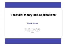
The behavior of particles larger than 100 µm in diameter is mainly controlled by gravity, that is, they do not tend to stick. This changes dramatically for particles less than 100 µm in diameter. Surface forces govern them. These forces can be a million times or more stronger than the gravitational pull and therefore these particles have a tendency to stick. As mentioned above, even though all surface forces are of electrodynamic origin, several interactions have specific names. First, we look into the most important and ubiquitous force responsible for sticking, the so-called van der Waals force. The origin of the theory on van der Waals forces dates back to the late 18th century. At that time the ideal gas equation was used to characterize and predict the behavior of every molecular or atomic gas. This approximation seemed to work well for monatomic gases like helium, xenon, and neon, as well as for simple diatomic gasses like Cl2 and H2. It seemed to fail though for compound gases with polar behavior, like H2O (Figure 11.1). In 1876 Johannes D. van der Waals ascribed this behavior to possible intermolecular interaction (despite the fact that the model of matter consisting of atoms was not accepted at that time) and suggested a modification to the well-established ideal gas equation known today as the van der Waals equation of state:1 (P /V2)(V ) = kBT
(11.1)
DK4027_book.fm Page 272 Friday, February 25, 2005 8:25 AM
272
Chemical Processing of Ceramics, Second Edition 1000
800
P (Atm)
600
400 (b) 200
(a)
0.2
0.4
0.6
0.8
1
Volume (lt)
FIGURE 11.1 Figure .showing (a) Van der Waals and (b) ideal gas equation for water. For Low energy (low pressure, high volume) the equations are similar, for high energy though there is a big difference.
Today, collectively those interactions are called van der Waals interactions. Electrostatic (coulomb) and hydrogen-bonding forces, however, are excluded from this group basically due to the nature of the force. The origin of the van der Waals forces is known to be electromagnetic, and more specifically, dipole interaction. All gases, despite the fact that they are neutral, might have a nonhomogeneous charge distribution (e.g., in water, the shared electrons are pulled closer to the oxygen than the hydrogen) and with the proper molecule structure (in water, the two hydrogen atoms and the oxygen atom form a 109.47° angle) can result in a dipole. Those dipoles produce vibrating electromagnetic waves and they interact with each other by inducing attractive or repulsive forces. By 1930 the dipole-dipole interaction had already been studied by classical physics and the interaction energy had been calculated to be W(r) = C/r6.
(11.2)
In the 1930s, Eisenschitz and London2 did analytical calculations with the perturbation theory in quantum mechanics and estimated the interaction energy between two induced dipoles as
()
3 1 W r = − α 20 I , 4 4 πε 0 r 6
(
)
(11.3)
DK4027_book.fm Page 273 Friday, February 25, 2005 8:25 AM
Theory and Applications of Colloidal Processing
273
Keesom interaction dipole-dipole
Debye interaction dipole-induced dipole
London interaction fluctuating dipole-induced dipole
FIGURE 11.2 The three major types of van der Waals interactions.
which is very similar to the classic expression, with the only difference being the numerical prefactor. The fluctuating dipole-induced dipole interaction is the strongest of the van der Waals interactions and is called a London interaction, but there are also dipole-dipole and dipole-induced dipole interactions that are called Keesom and Debye interactions, respectively (Figure 11.2). In 1937 Hamaker had the idea of expanding the concept of the van der Waals forces from atoms and molecules to solid bodies.3 He assumed that each atom in body 1 interacts with all atoms in body 2, and with a method known as pairwise summation, found an expression for the interaction between two spheres of radius R1 and R2:
( )
W d =−
A R1R2 , 6d R1 + R2
(11.4)
where A is a material constant, called the Hamaker constant, and depends on the geometry: A = 2C12.
(11.5)
This theory can be extended to several other geometries and many kinds of interaction can be predicted (Table 11.1). The major disadvantage of this microscopic approach theory was the fact that Hamaker knowingly neglected the interaction between atoms within the same solid, which is not correct, since the motion of electrons in a solid can be influenced by other electrons in the same solid. So a modification to the Hamaker theory came from Lifshitz in 1956 and is known as the Lifshitz or macroscopic theory.4 Lifshitz ignored the atoms completely; he assumed continuum bodies with specific dielectric properties. Since both van der Waals forces and the dielectric properties are related with the dipoles in the solids, he correlated those two quantities and derived expressions for the Hamaker constant based on the
DK4027_book.fm Page 274 Friday, February 25, 2005 8:25 AM
274
Chemical Processing of Ceramics, Second Edition
TABLE 11.1 Van der Waals Forces for Different Geometries Two atoms
( )
W D =−
Two Spheres
C D6
Atom surface
( )
W D =−
πC ρ 6D3
Parallel chain molecules
( )
W D =−
A R1R2 6 D R1 + R2
Sphere-Surface
( )
W D =−
AR 6D
Surface-Surface
( )
W D =−
A 12 πD 2
DK4027_book.fm Page 275 Friday, February 25, 2005 8:25 AM
Theory and Applications of Colloidal Processing
275
dielectric response of the material. The detailed derivations are beyond the scope of this book and readers are referred to other publications. The final expression that Lifshitz derived is
A132 =
3 k BT 2
∞
( )
( )
( ) ( )
∑ ( ) ( ) n= 0
( ) ( )
ε1 i νn − ε3 i νn ε 2 i νn − ε3 i νn , ε1 i νn + ε3 i νn ε 2 i νn + ε3 i νn
(11.6)
where the pointers 1, 2, and 3 refer to material 1 and 2 interacting in medium 3, and ε(v) is the dielectric permittivity of the material in frequency v. The expression, although it looks simple, is not easily calculated because there are complications in finding the dielectric permittivity in every frequency and is even more difficult at frequencies of zero and infinity. A simplification of this expression is to assume that the main contribution is coming from the ultraviolet (UV) and infrared (IR) part of the spectrum. Under this approach, the expression of the dielectric permittivity can be written as
()
ε ν = 1+
CIR CUV . + 1 − i ν ν IR 1 − i ν νUV
(11.7)
More approximations can be made from this point to further simplify the calculations, but all of them require experimental inputs at some point about the optical properties of the material. If the optical data of the materials are known, then the calculation of the Hamaker constant can be completed. At the frame of the Lifshitz theory, there is an important aspect to be noted. The Hamaker constant can be positive or negative5,6 depending on the materials, and sometimes even zero; something that has critical importance for colloidal stability, as will be explained later. This can be seen easier in the Tabor-Winterton approximation, which, starting from the Lifshitz theory, simplifies the Hamaker constant:7 A132 =
+
ε −ε ε −ε 3 k BT 1 3 1 3 4 ε1 + ε3 ε1 + ε3
(n
)( 2 n +n ( ) ( n + n ) {( n 2 1
3hνe 8
2 1
2 3
12
2 2
2 3
− n32 n22 − n32 12
2 1
+ n32
)
(11.8)
) + (n 12
2 2
+ n32
)
12
}
In the case where the medium and the solids have the same index of refraction (n1 = n2 and ε1 = ε2), the Hamaker constant A132 goes to zero. This method is known as index matching and is used to minimize or eliminate the effect of the Hamaker constant. Table 11.2 lists Hamaker constants for several materials.
DK4027_book.fm Page 276 Friday, February 25, 2005 8:25 AM
276
Chemical Processing of Ceramics, Second Edition
r R AU: Figure 11.3 is not called out in the text.
FIGURE 11.3 Principles of pairwise summation used by Hamaker.
TABLE 11.2 Isoelectric Point and Hamaker Constants in Vacuum and Water for Various Materials106 Material TiO2 SiO2 (amorphous) α-Al2O3 Si3N4 BaTiO3 ZnO
Hamaker Constant in Vacuum (10–20 J) 15.3 6.5 15.2 16.7 18 9.21
Hamaker Constant in Water (10–20 J)
Isoelectric Point
5.35 0.46 3.67 4.85 8 1.89
4–6 2–3 8–9 9 5–6 9
Figure 11.4 demonstrates the van der Waals forces for the system of aluminaalumina in water for three different particle radii. As mentioned earlier, the van der Waals interaction occurs due to the synchronization of dipoles. The electromagnetic field travels with the speed of light, so time is required for dipole synchronization. For long distances, the dipoles fail to synchronize properly so the effect is not as strong as predicted by the theory. This phenomenon is known as the retardation of van der Waals force or CasimirPolder8 correction and starts to be noticeable at distances greater than 5 nm. Similar decay of the van der Waals interaction can be observed in the case of two particles in a polar medium. In this case the free charges of the medium are screening the dipoles. This phenomenon is known as screened van der Waals force and is important in small distances, about half the Debye length, 1, the meaning of which is explained later in this chapter.
B. ELECTRIC DOUBLE LAYER FORCES For the processing of ceramics in liquids, it is important to introduce repulsive forces to overcome attractive van der Waals forces. One type of force is the socalled electric double layer (EDL) force. Some books refer to this force as electrostatic force. To avoid confusion, the term EDL force is used throughout this chapter to clearly show that the physics of particles in liquids strongly differs
DK4027_book.fm Page 277 Friday, February 25, 2005 8:25 AM
Theory and Applications of Colloidal Processing
277
2
0
R = 100 nm
−2
500 nm Wvdw −4 kB T
1 µm
−6
−8
0
0.2
0.4 0.6 Separation distance (µm)
0.8
1
FIGURE 11.4 Van der Waals energy for three sizes of spherical particles (Al2O3 in water). R = radius of the spherical particle. The ordinate is normalized by a Boltzmann factor to make for easy comparison to Brownian energy (EBr = 2/3 kb T).
AU: Table 11.3 is not called out in the text.
TABLE 11.3 The Debye Length as a Function of the Concentration for Different Types of Electrolyte 1/κ (nm)
0.304 AX 0.176 AX 2 0.152 A2 X 2
Electrolyte Valence For 1:1 electrolyte (NaCl, KCl)
For 2:1 electrolyte (CaCl2, Na2SO4)
For 2:2 electrolyte (CaCO3, MgSO4)
DK4027_book.fm Page 278 Friday, February 25, 2005 8:25 AM
278
Chemical Processing of Ceramics, Second Edition +
Counter ions
−
Adsorbed co-ions
Diffusion layer −
Solvent ions
+
+
+ −
+
− − +
+ −
+
Outer helmholtz plane Inner Shear plane helmholtz plane
−
−
Gouy plane
Bulk solution
FIGURE 11.5 Electric double layer (EDL). In this example: the surface selectively adsorbs negative ions and a second layer is formed from the counter ions.
from particles in air, where electrostatic forces apply that follow Coulombs law. This section describes the chemistry in the development of surface charges on particles and the physics equation that governs the forces. A perfect stoichiometric crystal with complete absence of defects is considered neutral, which implies that the surface will be neutral too, thus there is no net surface charge. This is true for diamond. As soon as the surface is oxidized, hydroxyl and other groups form that develop a charge as soon as it is immersed in a protic liquid. For any material, there are four major sources of this charge: ionization or dissolution of surface groups, specific ion adsorption, ion exchange, and solution of specific ions out of the surface. In 1901 Stern9 assumed that when particles are submerged in an electrolyte containing solvent, there is a second layer of charges with opposite sign (counter ions) formed on top of the first layer.10,11 Thus he called the system electric double layer (EDL) (Figure 11.5). Later Gouy12 and Chapman13 modified the Stern theory by assuming that the EDL is formed between the surface charge and a diffusion (buffer) layer that extends to a certain distance from the surface (a few nanometers).14 The EDL is creating a potential known as surface potential, and decays away from the surface. The general solution of this potential is given from the combination of two equations, the Poisson equation for the potential decay and the Boltzmann equation describing the statistical distribution of ions. The Poisson-Boltzmann equation, zeρ0 − zeΨ / kT d 2Ψ( x ) = − e , 2 εε 0 dx
(11.9)
DK4027_book.fm Page 279 Friday, February 25, 2005 8:25 AM
Theory and Applications of Colloidal Processing
279
does not have an analytical solution, but can be solved numerically for a specific case. A simplification of this is the Debye-Hückel15 equation, which assumes simple exponential decay: Ψ ( x ) = Ψ 0e − κx ,
(11.10)
where Ψ is the potential, Ψ0 is the value at the surface, and 1/κ is known as the Debye length, which physically gives the range of the field and is given as a function of the electrolyte concentration (ρ) and valence (z): 12
ε 0 εk BT 1κ= e2 ρi zi2 el i
∑
.
(11.11)
The measurement of this surface potential (Ψδ or Ψ0) is impossible due to the hydrodynamic behavior of the system that generates a thin layer of attached liquid around the particles. However, there is a plane where the shear starts (shear plane), and at this plane the surface potential can be measured and the value is known as the zeta (ζ) potential (Ψζ). Besides the indifferent counter- and co-ions in solution, there are also so-called potential determining ions (chemists call them adsorbing ions). For most systems these are H+ and OH ions that can adsorb directly on the particle surface and alter the ζ potential. There is a pH value for which the ζ potential becomes zero and is called the isoelectric point (IEP), as shown in Figure 11.6. For another pH value (usually very close to the IEP) there is the point of zero charge (PZC) where the surface potential becomes zero. For every application, the IEP and the PZC are to be the same, as well as Ψδ and the Ψζ. Increasing the concentration of an indifferent monovalent electrolyte in a solution will decrease the value of ζ potential and the Debye length, and eventually the EDL will collapse, but it will not change the IEP. For divalent electrolytes, however, and for high concentrations, the sign of the ζ potential can be reversed and the IEP is shifted. So, for example, if a gold surface, which is positively charged, is submerged in a Na2SO4 solution, the SO42 ions will adsorb on the surface, and if the concentration is enough, all the surface sites are covered. In this case there will be an excess of negative charge that will inverse the sign of ζ-potential. This change will shift the IEP because now the H+ ions and not the OH ions are the potential determining ions. If this happens, the ions are referred to as potential determining or specifically adsorbing. The surface charge is important for the colloidal stability because the induced entropic forces can separate or coagulate the particle suspension. For two particles of radius R1 and R2, the interaction energy is16 2
RR k T W d = 64 πε 0 εr γ 1γ 2 1 2 B e −κd , R1 + R2 ve
( )
(11.12)
DK4027_book.fm Page 280 Friday, February 25, 2005 8:25 AM
Chemical Processing of Ceramics, Second Edition
Zeta potential (mV)
280
80
80
40
40
pHIEP = 9.1 0
−40
0
2
3
4
5
6
7
8
9
10
−40 11
pH
FIGURE 11.6 Zeta potential as function of pH for Alumina (Al2O3).
where
(
γ i = tanh veΨ iδ 4 kB T
)
ε0 is the vacuum dielectric permittivity, εr is the medium dielectric constant, e is the elementary charge, and v is the number of electrons. For same-material particles, the force will always be repulsive, but the range will differ depending on the electrolyte concentration (Figure 11.7). For particles of different material or different surface chemistry that are in a medium at a pH that is between the two IEPs, then the ζ- potentials will have different signs, and thus the force will be attractive. For any other pH value, the force will be repulsive, but the magnitude will depend on the pH. It must be noted here that for very short distances (less than 10 nm), the surface charge interaction is very strong and it forces the charges to be redistributed on the surfaces, and while the separation distance approaches zero, the surface charge density becomes a function of the distance. This phenomenon is known as charge regulation17 and reduces the effective EDL stabilization.
C. COLLOIDAL STABILITY In 1942 Derjaguin and Landau18 and Verwey and Overbeek19 (DLVO) suggested that the total energy of a colloidal system is the summation of van der Waals and EDL interactions. For the case of spherical particles of radius R, this has the form 2
RR k T 6 R1R2 . W d = 64 πε 0 εr γ 1γ 2 1 2 B e − κd − 6 D R1 + R2 R1 + R2 ve 1444444 24444443 1442 44 3
( )
EDL
vdW
(11.13)
DK4027_book.fm Page 281 Friday, February 25, 2005 8:25 AM
Theory and Applications of Colloidal Processing
281
60
50
40 Vtot 30 kB T 20 0.001 M NaCl 10
0.01 M 0.1 M 0
10
20 30 Surface separation (nm)
40
FIGURE 11.7 Electric double layer interaction between two spheres of 100 and 500 nm, and for three different values of monovalent electrolyte (0.1 M, 0.01 M and 0.001 M), which results three different values for the EDL thickness (0.96 nm, 3.04 nm, and 9.61 nm, respectively).
In most cases of colloidal suspensions, the attraction part comes from van der Waals forces and repulsion comes from EDL forces. A graph of these interactions is shown in Figure 11.8, where, for specific parameters, a repulsive barrier is created. In order for the particles to coagulate they must overcome this barrier and reach the primary minimum. For small barriers, simple mechanical energy, like vibration, is enough to cause coagulation, but for larger barriers, addition of electrolyte or a shift in pH toward the IEP is usually used to collapse the EDL and destabilize the suspension. As shown in Figure 11.8, just before the barrier there is a small, but significant minimum where the system is stable and still at a significant separation distance. This is known as the secondary minimum, and at this point the system is weakly flocculated and only small energies are required to move it from this position.
D. COAGULATION KINETICS For the case where the system has no barrier, the primary minimum will cause two particles to coagulate every time they collide. This is known as fast coagulation, and since the sticking coefficient is almost one, the coagulation kinetics are governed by diffusion. According to the Smoluchowski20–22 theory of fast coagulation, the rate at which primary particles disappears is dn/dt = 8rcDn2
(11.14)
DK4027_book.fm Page 282 Friday, February 25, 2005 8:25 AM
282
Chemical Processing of Ceramics, Second Edition 50 40 30 C = 0.001 M NaCl (barrier) Vtot kB T
20 10
C = 0.02 M NaCl (secondary minimum)
0 −10
C = 1 M NaCl (primary minimum)
0
5
10 15 20 Surface separation (nm)
25
30
FIGURE 11.8 DLVO interaction for Al2O3 in water with three different electrolyte concentrations. For low electrolyte concentration the effective barrier can stabilize the particles at distance κ-1 (~9 nm). For larger concentrations a secondary minimum can cause weak coagulation of the suspension at the secondary minimum. Even higher concentrations can completely eliminate any repulsion (fast coagulation).
and the number of collisions per unit time is J = 4Drcn0
(11.15)
D = kT/6rc,
(11.16)
and the diffusion coefficient, D, is
where n is the number of primary particles (which have not yet coagulated), n0 is their number at t = 0, rc = 2R, and η is the viscosity of the system. An important parameter to characterize the coagulation kinetics is the time required for 50% coagulation and is calculated from the previous equation to be t1 2 =
1 . 8πrc Dn0
(11.17)
Typical values calculated from the previous equations are approximately 0.1 to 1 s. In reality, coagulation times are longer. This can be attributed to the fact that for large distances the solvent acts as a continuum medium, so the opposition of the medium to the particle movement is incorporated in the equations with the viscosity coefficient. However, for smaller separation distances the solvent cannot
DK4027_book.fm Page 283 Friday, February 25, 2005 8:25 AM
Theory and Applications of Colloidal Processing
283
be considered as a continuum any more. This results in a reduced diffusion coefficient for smaller distances. The analytical solution to this problem is very difficult; however, there are some empirical equations that can be used. The effective diffusion coefficient as a function of the separation distance r is23 Deff = D
6 x 2 − 20 x + 16 , 6 x 2 − 11x
(11.18)
where x = d/R. Even with this correction there is some deviation from the actual time, because the theory is neglecting the presence of particle clusters, although they are constantly forming via the collisions. In the case of energy barriers, the previous theory is not applicable anymore, since besides diffusion, the coagulation depends on the barrier threshold, too. The coagulation rate is expected to be less, and so it is called slow coagulation. The probability for the particles to overcome the barrier depends on the energy barrier (Eb) and the temperature according to the Boltzmann distribution, P ∝ e − Eb
k BT
.
(11.19)
So a reasonable modification of the disappearing rate equation, for the case of the slow coagulation will be dn = −8πrc Dn 2 e − Eb dt
kB T
.
(11.20)
The ratio between the two rates is called the stability ratio, W, and is W=
n& fast = e Eb n&slow
k BT
W =
η fast ηslow
= e − Eb
kB T
.
(11.21)
Still that theory is not fully satisfying because it does not include the particleparticle interactions, which in this case are long range (~1). A more accurate expression for the stability ratio for this case is d =∞
W = rc
1
∫ d e
( )
W d k BT
dd ,
(11.22)
d =2 R
which for the case of an EDL stabilized suspension can be approximated with 1 Eb / k B T W = e . κrc
(11.23)
DK4027_book.fm Page 284 Friday, February 25, 2005 8:25 AM
284
E. STERIC
Chemical Processing of Ceramics, Second Edition AND
ELECTROSTERIC FORCES
As seen in Figure 11.4, van der Waals forces are size and material dependent, so there are cases where the EDL barrier is too low to stabilize the colloid, especially when there is only a small potential (less than 15 mV) and high ionic strength involved. For those cases, other techniques, such as steric24 and electrosteric25 stabilization, have been developed. For steric stabilization, selected organic macromolecules—polymers— are added to the suspension. These molecules are designed to adsorb on the particle surface. In order to be a good dispersant the polymer has to adsorb on the surface and have good solubility in the dispersing medium. There are three main categories of theories that have been developed for polymers on surfaces for colloidal stabilization: mean field theories,26–31 scaling theories,32–34 and Monte Carlo theories.35–38 These theories have all been successfully applied to describe the impact on colloidal stability. It has been shown that mean field theories work best for polymers at the temperature, Monte Carlo for poor solubility and scaling theory for well-soluble polymers. Even though some theories, such as scaling theory, have been developed for endgrafted polymers on surfaces, they can be applied for adsorbed polymer layers. Since this theory applies to well-soluble polymers, that is, the polymer segment-solvent interaction is more favorable than the segment-segment interaction, a few quantitative formulas will be presented that apply to ceramic processing. The interaction of two adsorbed polymer layers in close proximity depends on the polymer solubility (polymer segment-solvent interaction), the surface coverage (adsorption density), as well as the chain length. At low polymer concentrations and with high chain length, one polymer chain can adsorb on more than one particle, and thus flocculate the system. This is referred to as bridging flocculation. At high polymer concentrations, that is, full polymer surface coverage of adsorption sites on the particle, the polymer can form two conformations: mushroom or brush.39–41 When polymer-coated surfaces come together the layers are forced to penetrate into other. The increase in segment density removes freedom of movement of the polymer chains, which results in a sudden drop in entropy. This is not a physically favorable process, so the particles cannot come closer than roughly twice the layer thickness. If the layer thickness is larger than the range of the van der Waals interaction, then it will act as an effective barrier, by preventing the coagulation, called steric stabilization. For layer thickness δ and separation distance 2δ > d > δ, the repulsive interaction is due to the layer mixing opposition and is equal to42
mix steric
V
(
)
32παk BT φ p 0.5 − χ d δ− d = 4 2 5vδ
( )
6
(11.24)
where v is the molar volume, χ is the Flory-Huggins parameter, and φ p is the average volume fraction of segments in the adsorbed layer. At smaller separation
DK4027_book.fm Page 285 Friday, February 25, 2005 8:25 AM
Theory and Applications of Colloidal Processing
285
distances, in addition to the mixing constraint, there is the elastic behavior of the layers, so the interaction is the summation of the two contributions:23
( )
( )
( )
mix elastic Vsteric d = Vsteric d + Vsteric d
(11.25)
where ρp is the density, and Mp is the molecular weight of the adsorbed polymer. There are five kinds of steric stabilizers: Homopolymers: Simple polymer chains that can adsorb on the surface and entropic repulsion stabilizes the particles. Branched polymers usually adopt more complicated conformations which results in a further entropy increase and more effective stabilization. Diblock copolymer: Where one block is strongly adsorbed on the surface and the other is extended into the solvent. Comb-like copolymer: A combination of two polymers, one that strongly adsorbs on the surface (train configuration) and acts as an anchored backbone for the other polymer to attach and extend into the solvent. Surfactants: Short chains consisting of an anchoring functional group and a short organic chain, usually hydrophobic or hydrophilic. Polyelectrolytes: Polymers that contain at least one ionizable group (i.e., carboxylic acid) such as polyacrylic acid (PAA). In the last case, the repulsion is even greater due to the strong long-range EDL repulsion between the charged molecules, known as electrosteric stabilization.43 In the case of high ionic strength, the polymer chains are neutral so they act like a polymer, and depending on the conditions they can have brush, pancake, or mushroom conformation. At low ionic strength, however, the charge is not screened and the electrostatic interaction among the chains pushes them to extend away from the surface, to brush conformation, or to adsorb flat in the pancake conformation if other interactions are stronger than the charge repulsion.
F. DEPLETION The origin of the depletion forces is attributed to a concentration gradient that may exist in the solution from the region around the particles to the region between the particles.44,45 This happens only for large particles (approximately 500 nm) and at the presence of a solute, known as depletant, usually polymer or nanoparticles (