Steven Brown, Frank Chance, Jennifer Robinson, and Rus- sell Barton. We thank Steven Brown for helping us under- stand backend manufacturing and for ...
Proceedings of the 2001 Winter Simulation Conference B. A. Peters, J. S. Smith, D. J. Medeiros, and M. W. Rohrer, eds.
IMPLEMENTATION OF RESPONSE SURFACE METHODOLOGY USING VARIANCE REDUCTION TECHNIQUES IN SEMICONDUCTOR MANUFACTURING Charles D. McAllister Bertan Altuntas Matthew Frank
Juergen Potoradi
Marcus Department of Industrial and Manufacturing Engineering The Pennsylvania State University University Park, PA 16802, U.S.A.
Infineon Technologies Advanced Logic SDN. BHD. Free trade zone Batu Berendam 75914 Melaka, MALAYSIA
complete, the wafers are sent to the backend process. The backend operations are comprised of three main facilities: Pre-assembly, assembly, and test/pack operations. After leaving the frontend process, the wafer is thinned in preassembly in order to fit in the required package. The back is covered with a thin coating of metal to allow attachment of the wafer to the package. The wafer is then scribed and separated into individual chips. The electrically functioning chips are selected and sent to an assembly operation (Aguilar 2000).
ABSTRACT Semiconductor manufacturing is generally considered a cyclic industry. As such, individual producers able to react quickly and appropriately to market conditions will have a competitive advantage. Manufacturers who maintain low work in process inventory, ensure that specialized equipment is in good repair, and produce quality products at least possible cost will have the best opportunities to effectively compete and excel in these challenging venues. To support this nimble business model, our current efforts are directed toward creating efficient, accurate metamodels of the impact of maintenance policies on production efficiency. These validated polynomial approximations facilitate rapid exploration of the design region, compared with the original simulation models. The experiment design used for metamodel construction employed variance reduction techniques. When compared to a similar experiment design using independent streams, the variance reduction approach provided a decrease in standard error of the regression coefficients and smaller average error when validated against the simulation response. 1
Figure 1: Silicon Ingot and Wafers This study covers the assembly portion of the backend operations. At the first assembly step, the chip is soldered or glued in the lead frames. Contacts on the dies are then wire-bonded to the leads. The thin gold or aluminum wires are typically 2.5 microns in diameter, and the package may have from eight to several hundred leads. The bonded chips are encapsulated in ceramic or mold compound to hermetically protect the die. The simulation model used in this study was supplied by one of the world’s largest semiconductor manufacturers, Infineon Technologies, originally a part of the Siemens Corporation. The model represents the Malacca Factory, which produces memory products. There are three product families:
INTRODUCTION
1.1 System Description Semiconductor manufacturing is one of the world’s most rapidly developing and growing industries. Manufacturing of semiconductors consists of two consecutive main operations which are called frontend and backend. The base for most semiconductors today is silicon, which is simply the main element found in sand. Basically, the frontend is the manufacturing of silicon-wafers used to produce the semiconductors. Figure 1 shows a silicon ingot with the slices from it, which will be silicon wafers after patterns are printed and etched on it. After all wafer-level processing is
•
1225
16M SS8 P-TSOPII-50-1: 0.25 micron process 16 megabit SDRAM
McAllister, Altuntas, Frank, and Potoradi •
64M S20 P-TSOPII-54-1: 0.20 micron process 64 megabit SDRAM 256M S20 P-TSOPII-54-1: 0.20 micron process 256 megabit SDRAM
•
DB1
The simulation model contains five different products each of which is a member of one of the above mentioned product families. These five products are distinguished by different processing times and different dedicated tools. These products are: • • • • •
DB2
WB6
WB1
WB7
WB2
Tsop54_ss4_x4 Tsop54_ss4_x8 Tsop54_ss4_x16 Tsop54_256M Tsop54_S19_x8
WB5 WB8
WB3
WB9
WB4
In the assembly area all five products follow the same process flow. The process flow chart of the assembly operations is provided in Figure 2. The flow contains ten main steps: die bonding, wire bonding, prebake, molding, post mold cure, dedam/dejunk, plating, trim and form, PC by off, and packing.
Key: DB WB
diebonder wirebonder
Figure 3: Autoline Configuration 1.2 Measures of Performance and Key Variables
TSOP54_SS4_x4, TSOP54_SS4_x8 TSOP54_SS4_x16, TSOP54_S19_x8
Diebonder_1 wirebonder_1
TSOP54_256M
1.2.1 Model 1
Diebonder_2
wirebonder_12
wirebonder_2
Split lots region
Diebonder_3 wirebonder_3
50Kbuffer
Diebonder_11
wirebonder_34
5%
95%
Ams_36
Ams_24 Pcs_oven
Ams_312
Bake_oven
Molding
1.2.2 Model 2
Post mold cure
Taf-1a
Dedam dejunk
Msts-1
Plating
Tmf-2a
Trim and form
Pc
Initial analysis efforts revealed that the processing time of the molding machines and the time between releases were significant determinants of system performance. We used both to predict work in process (WIP).
wirebonder_11
To optimize Model 1, one would minimize WIP by maximizing the time between releases and minimizing the processing time. Due to the practical limitations of Model 1, we also considered a cost model. The decision variables in this model were the time between, and duration of, both scheduled and unscheduled maintenance. These variables have an effect on both WIP and Cycle Time, which are performance measures used to calculate cost per part in the objective function.
Packing
Test
Figure 2: Process Flow Diagram As seen in the flow chart of Figure 2, there are 11 parallel lines, each of which has a diebonder and a number of wirebonders. These lines are called autolines, and the configuration is depicted in Figure 3. The configuration depends on the number of the diebonders and the wirebonders. One autoline can have up to two diebonders and 10 wirebonders. As shown in Figure 3, some of the autolines share one wirebonder. The initially formed product lots are split into magazines before going into the autolines and combined after the post mold cure operation. The default magazine size is 480 units for all of the products (Potoradi 2000).
1.3 Optimization When the objective to be optimized depends on a complex model, one can use Response Surface Methodology (RSM) (Neddermeijer et al. 2000; Myers and Montgomery 1995; Barton 2000). The steps of RSM are presented in Figure 4. At the core of this process is the fitting of a full quadratic model and is the focus of our study.
1226
McAllister, Altuntas, Frank, and Potoradi Hence, we seek negative correlation between Y~1 and Y to reduce the variance. (Schmeiser 1999). To induce this correlation structure, we use complementary random numbers. If random number U is used for a particular purpose in the model, we use 1-U for this same purpose in the second run. The use of common random numbers is restricted to comparisons of two or more alternative system configurations. Considering responses Y1 and Y2 from two configurations, ~2
Var (Y1-Y2) = Var(Y1) + Var(Y2) – 2Cov(Y1, Y2)
If the simulations are conducted with different random numbers, the two configurations will be independent. Hence, Cov(Y1, Y2) = 0. However, if we can induce a positive correlation between Y1 and Y2, then Cov(Y1, Y2) > 0, and we will have reduced the variance of (Y1-Y2) in Equation (2) compared to the independent configurations. Hence, we seek positive correlation between Y1 and Y2 to reduce the variance. We attempt to induce this correlation by using the same random numbers to simulate each configuration. Further, these random numbers must be synchronized for use in the same purpose within every configuration. Law and Kelton (2000, pp. 586) summarize, “Ideally, a specific random number used for a specific purpose in one configuration is used for exactly the same purpose in all other configurations.” For example, if a particular random number is used to generate the arrival time of a lot of chips to backend assembly, then it should be used in future configurations to generate the same arrival time rather than for the generation of a processing time or other purpose. If we cannot ensure this synchronization, the full benefit of CRN will be lost. Despite concerted effort, it is possible that a CRN implementation will lead to an increase in variance of (Y1Y2) by causing negative correlation. Therefore, validation is required.
Figure 4: Response Surface Methodology 1.4 Purpose of the Paper This paper shows the application of RSM technology to a backend assembly maintenance decision. A variance reduction technique was employed to observe its impact on the precision of the metamodels. Towards this end, we present the implementation of RSM using variance reduction in Section 2. The results of this approach are outlined in Section 3, while recommendations are presented in Section 4. 2
RESPONSE SURFACE MODELS
2.1 Variance Reduction Techniques Using antithetic variates to reduce the variance of a single system, we seek to induce negative correlation between separate simulation runs. In this way, a small observation in one run is offset by a large observation in the complementary run. Taking the average of the pair, it will tend to be closer to the common expectation m of an observation than if the two observations were generated independently (Law and Kelton 2000). We observe a pair of responses Y~1 and Y~2 where Y~2 is the obtained from the properly synchronized antithetic run corresponding to Y~1. We take the average of these two responses as the estimate of the true performance mean. Then, Y ~1 + Y ~ 2 Var 2
(2)
2.2 Factory Explorer Implementation Antithetic variate implementation in Factory Explorer was accomplished with a beta version of the software. It contains a run option that allows the user to specify antithetic random numbers for a given starting stream. Using a common random number scheme in Factory Explorer involved assigning a separate random number stream to each source of variation in the backend assembly model. By dedicating streams to specific purposes, we have a much better chance of using the same random numbers for the same purpose as the system configuration is altered. As explained by the Factory Explorer documentation (1995), the synchronization of the random number streams gradually degrades with multiple replications. The rec-
Var (Y ~1 ) + Var (Y ~ 2 ) + 2Cov(Y ~1 , Y ~ 2 ) (1) = 4
1227
McAllister, Altuntas, Frank, and Potoradi part cost is a summation of the components of production cost divided by the total production volume in a unit period. The four terms in this cost function are: manufacturing cost, inventory cost, unscheduled maintenance cost, and scheduled maintenance cost. Manufacturing cost, Mc, as defined above is the manufacturing cost per day of the backend assembly. The total inventory cost is calculated by a product of the per part daily inventory holding cost and average daily work in process for a given run length. Unscheduled and scheduled maintenance costs are determined in a similar manner; labor rates are multiplied by the total required maintenance time. There is a perceived inverse relationship between the amount of scheduled maintenance and the subsequent occurrences of unscheduled maintenance required. This is captured through Equations (3) and (4) where, as the time between scheduled maintenance increases over the nominal time, the frequency and duration (1/Tu and Du, respectively) of unscheduled maintenance will increase.
ommended remedy is to specify an arbitrary stream offset. Suppose we choose an offset of 500 and consider any one random number stream. Then, when the first replication is complete, the stream would effectively be “rewound” to begin at the 500th random number obtained in the first replication. The documentation describes this as resetting the synchronization. We implemented this offset refinement to CRN in our models with an arbitrary value of 100. 2.3 Use of the Schruben-Margolin Design The Schruben-Margolin experimental design as shown in Figure 5 is based on a central composite design (Schruben and Margolin 1978). Ts
Key: Ts: Time between scheduled maintenance
Ds: Duration of scheduled maintenance Common Random Number Streams
Ds
Table 1: Cost Model Components
Antithetic to
Quantity Cp: Cost/part Du: Duration of unscheduled maintenance Ds: Duration of scheduled maintenance Dso: Initial duration of scheduled maintenance Tu: Time between unscheduled maintenance Ts: Time between scheduled maintenance Tso: Initial time between scheduled maintenance TTu: Total unscheduled maintenance time TTs: Total scheduled maintenance time Mu: Unscheduled maintenance cost rate Ms: Scheduled maintenance cost rate Ic: Inventory holding cost CT: Cycle Time WIP: Work in Process TP: Throughput Mc: Manufacturing cost of back-end factory RL: Simulation run length
Independent Stream Antithetic to
Figure 5: Schruben-Margolin Graphical Design It incorporates variance reduction techniques in the following manner. Corner points are run using a common random number strategy. Axes points are antithetic runs corresponding to the corner points. Typically, there are antithetic and independent runs made at the center to aid the estimation of lack of fit. Compared to the use of common random numbers for all points, the Schruben-Margolin approach reduces the bias of the fitted model coefficients. Compared to a corresponding design made only with independent streams, the Schruben-Margolin design results in decreased standard errors of the fitted model coefficients (Schruben and Margolin 1978). A rotatable central composite design formed the basis of our particular Schruben-Margolin implementation. Thus, axes and corner points were equidistant from the center of the design. Geometrically, this distance was sqrt(2)*design range/2. Four independent runs were made at the center with two additional antithetic replications corresponding to two of the independent runs.
Units $/part days days days days days days days days $100/hour $100/hour $1/part/day hours/part parts/day parts/day $150,000/day days
TTs = RL(Ds/Ts) TTu = RL(Du/Tu) Tu = Tuo + (Tso – Ts) + (Ds – Dso) Du = Duo + .01(Ts – Tso) + (Dso – Ds)
(3) (4)
Cp = (Mc+Ic*WIP*RL+Mu*TTu+Ms*TTs)/(TP*RL)
(5)
2.5 Experiment Designs and Implementation A summary of the experimental approach is depicted by Figure 6. For a Schruben-Margolin design on time between scheduled maintenance (Ts) and duration of scheduled maintenance (Ds), the simulation runs were made to observe the corresponding factory performance characteristics. We used the resulting data to calculate the cost per
2.4 Key Factors and Objectives Derivation of the objective function is summarized by Table 1. A cost model was developed to capture the effect of model changes on the cost per part, Equation (5). This per
1228
McAllister, Altuntas, Frank, and Potoradi Table 2: Schruben-Margolin vs. Independent Stream Designs for Model 1 Standard Error Independent Schruben-Margolin Coefficient INT 9321 8832 PTM 14181 13437 TBR 14181 13437
part according to the cost model and fit a polynomial metamodel for use with Response Surface Methodology. WIP CT TP
Back-end Factory Simulation
Ts Ds 2-Factor Schruben-Margolin
Polynomial Response Surface
Table 3: Schruben-Margolin vs. Independent Stream Designs for Model 2 Standard Error Independent Schruben-Margolin Coefficient INT 6.306 3.000 Ts 8.526 4.056 Ds 8.526 4.056 Ts*Ds 5.265 2.505 Ts*Ts 3.932 1.871 Ds*Ds 3.932 1.871
Cost Model
Ts* Ds*
Figure 6: Experimental Procedure 3
RESULTS
The Schruben-Margolin design was used in the analysis for two reasons. First, we wanted to explore the ramifications of using a design strategy based on variance reduction techniques in Response Surface Methodology. Secondly, this design, in theory, reduces the error in the regression models. To validate this premise a study was conducted to compare the Schruben-Margolin design with a design that only used independent random number streams. The validation was conducted for both models used in this study, time between releases (TBR) and processing time of the bottleneck molding machines (PTM) as determinants of WIP, and time between scheduled maintenance (Ts) and duration of scheduled maintenance (Ds) as predictors of cost. The same central composite design that was used in the first iteration of each optimization was run using only independent random number streams. Then, a first order regression model was fit for Model 1, and a full quadratic was fit for Model 2. Standard errors were computed for the coefficients of the regression model created using the Schruben-Margolin design and the independent stream design. The results provided in Tables 2 and 3 show the standard error is less for the coefficients generated by the Schruben-Margolin design for both models. We conclude that the use of Schruben-Margolin design provides a model with less error and therefore, creates a more accurate model. Figure 7 presents a graphical representation of one of the response surfaces generated through RSM using a full quadratic model of time between and duration of scheduled maintenance to predict the cost per part. As depicted, the normalized search direction to minimize the unit cost is (+1, +1).
1.8
1.7
Cost 1.6 0.95 0.85 0.65
0.75
Ds
0.75 0.85
0.95
Ts
0.65
Figure 7: Predicted Response of Cost vs. Duration and Time Between Scheduled Maintenance for a Quadratic Model Fit During RSM Implementation 4
RECOMMENDATIONS
With respect to the semiconductor manufacturer, it appears that a reduction in time between and duration of scheduled maintenance could yield a reduction in cost per part. From the results of the RSM implementation, a 10-15% reduction would be appropriate. Metamodeling efforts using the variance reduction techniques led to a decrease in standard errors of the fitted regression model coefficients compared to a similar design implemented with independent replications. Further, the Schruben-Margolin design had lower average absolute error when validated against the simulation response. In closure, it would be advisable to use common random numbers and antithetic variates in RSM.
1229
McAllister, Altuntas, Frank, and Potoradi Schruben, L.W. and B.H. Margolin. 1978. Pseudorandom number assignment in statistically designed simulation and distribution sampling experiments. Journal of the American Statistical Association 73, 504-525.
ACKNOWLEDGMENTS We gratefully acknowledge the assistance and insight of Steven Brown, Frank Chance, Jennifer Robinson, and Russell Barton. We thank Steven Brown for helping us understand backend manufacturing and for spending many hours in consultation and travel on this project. We appreciate the Factory Explorer assistance provided by Frank Chance and Jennifer Robinson, with particular recognition for the beta version that incorporated antithetic random variates. We acknowledge the insight and constructive comments provided by Russell Barton.
AUTHOR BIOGRAPHIES CHARLES D. MCALLISTER is a pursuing a Ph.D. in Industrial Engineering and Operations Research at Penn State. He is supported by a graduate fellowship from the Office of Naval Research and maintains research interests in stochastic multidisciplinary design optimization and simulation modeling. He received his B.S.I.E (Honors; Distinction) at the University of Nebraska and M.S.I.E. from Purdue University. His email address is .
REFERENCES Aguilar, R. A. 2000. Assembly and Test Process Overview. Internet document, , Arizona State University. Barton, R. R. 2000. IE 578: Using Simulation Models for Engineering Design. Fall semester lecture notes, The Pennsylvania State University. Factory Explorer User Manual. 1995. Pleasanton, CA: Wright Williams & Kelley. Grewal, N.S., A.C. Bruska, T.M. Wulf, and J.K. Robinson. 1998. Integrating Target Cycle-Time Reduction into the Capital Planning Process, Proceedings of the 1998 Winter Simulation Conference, eds. D.J. Medeiros, E.F. Watson, J.S. Carson and M.S. Manivannan, 10051010. Piscataway, New Jersey: IEEE Press. Law, A. W. and W. D. Kelton. 2000. Simulation Modeling and Analysis (3rd ed.). New York: McGraw-Hill, Inc. Murray, S., G.T. Mackulak, J.W. Fowler, and T. Colvin. 2000. A Simulation-Based Cost Modeling Methodology for Evaluation of Interbay Material Handling in a Semiconductor Wafer Fab, Proceedings of the 2000 Winter Simulation Conference, eds. J.A. Joines, R.R. Barton, K. Kang and P.A. Fishwick, 1510-1517. Piscataway, New Jersey: IEEE Press. Myers, R.H. and D.C. Montgomery. 1995. Response Surface Methodology: Process and Product Optimization Using Designed Experiments. New York: Wiley. Neddermeijer G. H., G.J. van Oortmarssen, N. Piersma and R. Dekker. 2000. A Framework For Response Surface Methodology For Simulation Optimization, Proceedings of the 2000 Winter Simulation Conference, eds. J.A. Joines, R.R. Barton, K. Kang and P.A. Fishwick, 129-135. Piscataway, New Jersey: IEEE Press. Potoradi, J., 2000. Documentation of Simulation Model for Semiconductor Backend Manufacturing, Technical Paper, Infineon Technologies, Inc. Schmeiser, B. W. 1999. IE 581: Simulation Design and Analysis. Spring semester lecture notes, Purdue University.
BERTAN ALTUNTAS is a Master’s Student in the Department of Industrial and Manufacturing Engineering at PSU, specializing in automated manufacturing systems. Mr. Altuntas received his B.S.I.E. from the Middle East Technical University, Turkey. His email address is . MATTHEW FRANK is a Ph.D. Student in the Department of Industrial and Manufacturing Engineering at PSU, specializing in integrated product and process design. Mr. Frank received his B.S.M.E and M.S.M.E from Penn State University. His email address is and his web page address is . JUERGEN POTORADI is a Production Control Manager with Infineon Technologies (formerly Siemens Semiconductor Division). He is currently responsible for the short term planning and logistics in a backend factory in Malaysia. Before, he was a Factory Modeling and Simulation analyst and project leader for implementing simulation techniques and methodologies in Singapore and Malaysia. Mr. Potoradi received his undergraduate and graduate degrees in Computer Science from the University of Wuerzburg in Germany. He has extensive experience in simulation analysis of semiconductor wafer fab and backend production operations. His email address is .
1230