Mirko Eickhoff. LS Informatik IV. Universität Dortmund. D-44221 Dortmund, GERMANY. ABSTRACT. In steady-state simulation the output data of the transient.
Proceedings of the 2003 Winter Simulation Conference S. Chick, P. J. Sánchez, D. Ferrin, and D. J. Morrice, eds.
TRUNCATION POINT ESTIMATION USING MULTIPLE REPLICATIONS IN PARALLEL Falko Bause Mirko Eickhoff LS Informatik IV Universität Dortmund D-44221 Dortmund, GERMANY
determine this distribution or derived measures. In practice, the calculation of F(x) is only possible for special cases, because the output process might never reach steadystate in finite time. By eliminating the transient phase, the steady-state distribution or derived measures are estimated on the basis of the observations xl+1 , . . . , x n , hopefully giving results close to the theoretical steady-state distribution. In the following we will call the observations xl+1 , . . . , x n the steady-state phase. In the literature the steady-state phase is, e.g., defined by the remark "relatively free of the influence of initial conditions" (Fishman 2001) or by the remark X l+1 , X l+2 , . . . X n "will have approximately the same distribution" (Law and Kelton 2000). These definitions are not precise enough for an algorithmic detection of the truncation point l and the practical knowledge of the analyst is still very important. It is therefore not much surprising, that the most common methods for detection of the truncation point are based on a visual inspection of the output data. Other, completely algorithmic methods give only proper results under special conditions (see (Gafarian, Ancker, and Morisaku 1978)) and are mostly based on one long simulation run. Nearly all methods use as a criterion convergence of the mean, although the steady-state phase is defined by the convergence of F j (x|S(0)) towards the steady-state distribution F(x). In this paper we focus on the output analysis of MRIP. One main advantage of k independent replications is, that it is possible to get k random values of F j (x|S(0)) and thus an estimation of the CDF of F j (x|S(0)). The accuracy of this estimation increases with an increasing number of replications. A significant advantage of MRIP is that the execution of k replications in parallel needs about the same amount of time than one single simulation run (provided we use, e.g., k computers), but gives more data for a better estimation of F j (x|S(0)). Since the prices of hardware are decreasing and performance is increasing, the execution of MRIP becomes a feasible method in practice.
ABSTRACT In steady-state simulation the output data of the transient phase often causes a bias in the estimation of the steadystate results. A common advice is to cut off this transient phase. Finding an appropriate truncation point is a wellknown problem and is still not completely solved. In this paper we consider two algorithms for the determination of the truncation point. Both are based on a technique which takes the definition of the steady-state phase more closely into consideration. The capabilities of the algorithms are demonstrated by comparisons with two methods most often used in practice. 1
INTRODUCTION
The output process {X j }nj =1 of a discrete-event simulator is influenced by the initial state S(0) chosen by the analyst. In general this influence is significant in the beginning and decreases with increasing model time. If one is interested in the steady-state behavior of the model, this initialization bias is obviously undesirable. A common way to reduce the influence of S(0) is to truncate the “most” influenced observations x 0 , . . . , xl−1 . Following this strategy the problem is to find an appropriate truncation point l. Many detection rules and methods can be found in the literature. Some are based on one simulation run (see (Pawlikowski 1990)) and some employ many independent simulation runs starting with the same initial state (cf. (Fishman 2001, Welch 1983)). The latter approach is called multiple (independent) replications in parallel (MRIP, see (Ewing, Pawlikowski, and McNickle 1999)) and will be considered in this paper. Let F j (x|S(0)) := Pr[X j ≤ x|S(0)] denote the cumulative distribution function (CDF) at model time index j . Assuming an ergodic system we have F j (x|S(0)) → F(x) if j → ∞. F(x) is called the steady-state distribution and the primary concern of steady-state simulation is to
414
Bause and Eickhoff 2.2 Method of Welch
(a) Linear Transient Mean
(c) Exponential Mean
Transient
(e) Periodic
The method of Welch extends the method of Fishman. It is based on the following experiences. The random error appears as a high-frequency oscillation in the sequence of column averages whereas the systematic error is in most cases a low-frequency oscillation. A sliding window comprising a sequence of column averages might be able to reduce the effect of the random error. Given a particular window size we can define an overall average from these column averages. Since the window is moving this average is called the moving average and sliding of the window results in a sequence of such moving averages. In practice, this sequence often seems to converge after some point l giving the wanted truncation point. For details see (Law and Kelton 2000, Welch 1983). 1. Compute {x¯ j }nj =1 . 2. Move a window of size w = 2K +1 across {x¯ j }nj =1. Calculate and plot the average of the interval in each single step. In order to avoid conflicts at the beginning, one starts with a window of size 1 (K = 0), which is increased until the desired size w is reached. After that, the window size is kept constant. 3. As long as the plot is not smooth, increase the window size by some value v > 0 and repeat step 2 with w := 2(K + v) + 1. As mentioned, the methods of Fishman and Welch require interaction of an experienced user. In the following we introduce two algorithms which need less user interaction. In practice, different situations might be encountered. On the one hand, one might has to deal with a static set of data, e.g., if the simulation has been terminated. On the other hand, one might be confronted with a dynamic set of data. E.g., if analysis of the output data is performed on-the-fly, additional data will become available during the simulation experiment. The following two algorithms take these two possible scenarios into account. One algorithm deals with a static set of data, the other deals with a dynamic set of data. Both aim at the detection of the truncation point l and are based on convergence characteristics of the empirical CDF of the random samples of X i .
(b) Linear Transient Variance
(d) ARMA(5, 5)
(f) Non-ergodic
Figure 1: PDF Over Time: Abscissa Represents Index of Model Time; Ordinate Shows Range of Y Divided Into Equally Spaced Y-intervals (A Dark Gray Point at Interval v Represents a High Probability of [Yt ∈ v], while a Light Gray Represents a Low Probability) 2
MULTIPLE REPLICATIONS IN PARALLEL
Let F˜ j (x|S(0)) denote the empirical CDF of the k values from the independent replications. F˜ j (x|S(0)) is an estimation of F j (x|S(0)) and, of course, the accuracy of this estimation increases with increasing k. Let x i, j denote the j th observation of the i th replication with 1 ≤ i ≤ k and 1 ≤ j ≤ n. If all x i, j are observations of the same measure and all x 1, j , . . . , x k, j are observed at the same model time or event, than the sequence {x i, j }ki=1 can be considered as an P independent random sample of X i . Let x¯ j = 1k ki=1 x i, j denote the column average. 2.1 Method of Fishman It is the nature of simulation that all estimated measures have a random error. In addition, measures might have a systematic error caused by the transient phase. This systematic error is known as the initialization bias and Fishman’s advice to detect it, is to examine the sequence of column averages {x¯ j }nj =1 (cf. (Fishman 2001)). Increasing the number of replications k decreases the random error, but the systematic error remains unaffected. 1. Compute and plot {x¯ j }nj =1 . 2. If the graph does not show a suitable “warm-up interval”, increase n and goto step 1.
3
415
STATIC DATASET
Assume that F˜n (x|S(0)) is the latest estimation of the steadystate distribution F(x), because the simulation terminated at model time index n. In order to find a proper truncation point, the first model time index l must be detected such that F˜ j (x|S(0)) ≈ F˜n (x|S(0)) for all j > l. One measure for equality of two random variables is the maximum difference of their empirical CDFs. The maximum difference of two CDFs X 1 and X 2 is given by maxx |F1 (x) − F2 (x)| where Fi (x) is the proportion of X i values less than or equal to x.
Bause and Eickhoff 10
10
column average
6
Fishman
4 2
6
2
0
0 -2 50
100 150 200 time index
250
300
0
(a) { x¯ j }nj =1 (Fishman)
rejections "a" (probability)
0.8 0.6
ASD 0.4 0.2 0 0
50
100 150 200 time index
250
50
100 150 200 250 time index (welch)
4.1 Algorithm for a Dynamic Dataset (ADD)
300
1.
(b) Moving Average (Welch; w = 11)
300
(c) Normalized Number of Rejections of Null Hypothesis (ASD) Giving l = 95
rejections of null hypothesis
1
Welch
4
-2 0
rejections of null hypothesis
The decision whether to terminate or to continue the simulations can be based on specific analysis results. Thus the set of data is now not limited a priori and its size varies dynamically with proceeding execution of the simulations.
moving average (w = 11)
8 measure
measure
8
1
2.
rejections "p" (probability)
3. 4.
0.8 0.6
ADD
n Compare T S with {x i, j }ki=1 for j = r+1 +1, . . . , n using the Kolmogoroff-Smirnov two-sample test. If more than ( p ∗ 100)% of the compared random samples {x i, j }ki=1 have a different probability distribution than T S: goto 2. n . Otherwise terminate with l := r+1 In (Bause and Eickhoff 2002) this algorithm for a dynamic dataset (ADD) was first introduced. Similar to ASD, this algorithm is based on the maximum difference of the empirical CDFs. ADD divides the observed random samples into three parts. The first part comprises the random samples, which have been assigned to the transient phase. The second part is the random sample, denoted as the testsample T S, which is tested whether it is a proper estimation for l. Finally, the third part are those random samples, which are assumed to be in the steady-state phase. This last part might be used to estimate F(x). Note that n is not bounded and therefore the algorithm need not terminate, which, e.g., might happen in case of a non-stationary model. Since the analysis can be performed in parallel to the simulation, the algorithm might be employed to determine a suitable stopping criteria for the simulation (cf. (Bause and Eickhoff 2002)). One key property of ADD is, that it preserves a predefined ratio of 1 : r between the transient and the steady-state phase, following an advice of Law and Kelton (Law and Kelton 2000). Surely, a proper choice of r depends on the model. Our experiences show, that r = 10 is a proper choice for many datasets and we used this choice in the following experiments. Testing whether two random samples originate from the same distribution is again performed using the KolmogoroffSmirnov two-sample test. Selecting this test seems reasonable, since it makes no assumptions on the distribution of the X j . When using ADD we selected an α-level of 0.05 and also set p to 0.05.
5.
0.4 0.2 0 0
50
100 150 200 time index
250
300
(d) Normalized Number of Rejections of Null Hypothesis (ADD) Giving l = 99
Figure 2: Plots of a Linear Transient Phase (Yt(1)) Given two empirical CDFs by two samples, the maximum difference can be determined by sorting these samples and comparing indices of corresponding X-values. All this gives the following algorithm. 3.1 Algorithm for a Static Dataset (ASD) Calculate F˜ j (x|S(0)) for 1 ≤ j ≤ n by sorting {x i, j }ki=1 . 2. Compute the maximum differences {d j }n−1 j =1 of ˜ ˜ F j (x|S(0)) and Fn (x|S(0)). 3. Compute for all j with 1 ≤ j ≤ n−1 the number of differences which miss the threshold in the interval [ j, n − 1]. 4. Choose l to be the minimum value of j after which only (a ∗ 100)% of the d j , d j +1 , . . . , dn−1 exceed the threshold z 2,k;1−α . The threshold z 2,k;1−α is the same threshold used in the Kolmogoroff-Smirnov two-sample test. Values of the threshold are tabulated. For details see (Hartung, Elpelt, and Klösener 1985). In our experiments we used an α-level of 0.05 and set a = 0.02. 1.
4
Choose a ratio 1 : r , and a level p, 0 ≤ p ≤ 1. Initialize n := 0 Observe r + 1 new X-intervals of all replications and compute the r + 1 new random samples: {x i,n+1 }ki=1 , . . . , {x i,n+r+1 }ki=1 Set n := n + (r + 1) n }k Set T S := {x i, r+1 i=1
DYNAMIC DATASET
Analysis of the output data parallel to the execution of the numerous simulations in the MRIP approach has some advantages. Most important is that the analysis process has the opportunity to guide the execution of the replications.
5
EXPERIMENTAL COMPARISON
As mentioned, it is well-known that a proper estimation of the truncation point has a significant impact on the quality of
416
Bause and Eickhoff
Fishman 0
Welch 0
-5
-5
-10 50
1
100 150 200 time index
250
300
0
rejections of null hypothesis
0
rejections "a" (probability)
0.8 0.6
ASD 0.4 0.2 0 0
50
100 150 200 time index
250
300
50
1
100 150 200 250 time index (welch)
300
rejections "p" (probability)
0.8 0.6
ADD 0.4 0.2 0 0
50
100 150 200 time index
250
10 9 8 7 6 5 4 3 2 1 0 -1
column average
Fishman
0
rejections of null hypothesis
-10
rejections of null hypothesis
measure
5 measure
measure
5
moving average (w = 101)
300
measure
10
column average
50
1
100 150 200 time index
250
rejections "a" (probability)
0.6
ASD 0.4 0.2 0 50
100 150 200 time index
250
moving average (w = 11)
Welch
0
0.8
0
10 9 8 7 6 5 4 3 2 1 0 -1
300
rejections of null hypothesis
10
300
50
1
100 150 200 250 time index (welch)
300
rejections "p" (probability)
0.8 0.6
ADD 0.4 0.2 0 0
50
100 150 200 time index
250
300
Figure 3: Plots for a Constant Mean with a Transient (2) Variance (Yt ) – ASD Gives l = 87 and ADD l = 91
Figure 4: Plots of an Exponential Transient Phase (3) (Yt ) – ASD Gives l = 149 and ADD l = 115
the simulation results (cf. (Fishman 2001, Law and Kelton 2000, Welch 1983)). Gafarian, Ancker and Morisaku define quality in more detail by attributes like accuracy, precision and generality (see (Gafarian, Ancker, and Morisaku 1978)). Here we want to deal with the quality in a more general view and test ASD, ADD and the methods of Fishman and Welch on some typical attributes of the output data of common models. In the following examples we use output data, that is not taken from simulations of "real" models. Instead we employ some well-known artificial processes with known properties. Especially characteristics of the truncation point are known in advance giving a precise criterion for comparison. We used the random number generator described in (L’Ecuyer, Simard, Chen, and Kelton 2002) and some additional transformations, described below. Let {�t }∞ t =1 denote an independent Gaussian white noise process (Hamilton 1994). This process is transformed into six processes with different attributes. In the following we employ k = 100 independent replications for each process.
f t is defined such that the transient phase ends at index l and Y (1) is the white noise process beyond index l. The parameter x describes the offset. Figures 2(a)- 2(d) show results obtained from applying the methods of Fishman and Welch, ASD and ADD for x = 10 and l = 100. As depicted, all methods give a good estimation of l. In Fig. 2(c) a cross represents the percentage of all dh with j ≤ h ≤ n − 1, which exceed the threshold z 2,k;1−α . In Fig. 2(d) a cross represents the normalized result of all performed Kolmogoroff-Smirnov two-sample tests at one step of the ADD. Normalization is done with respect to all tests, i.e. the normalized number of rejections of the null hypothesis is plotted. At about t = l we find the first random sample being (approximately) equal to all remaining random samples. Obviously, due to randomness some “outlier” test samples still show differences, but the algorithm determines the truncation point accurately near t = 100.
5.1 Linear Transient Mean
The second considered process (see Fig. 1(b)) has a constant mean, but there is a transient behavior of the variance.
(1)
5.2 Linear Transient Variance
The first inspected dataset (see Fig. 1(a)) is a realization of the process (1)
(1)
= ft
Yt
+ �t . (1)
A transient phase originates from f t ( (1)
ft
=
x −t 0
x l
(2)
Yt
(2)
= ft
· �t
(3)
(1) (
which is defined as
if t < l, else.
f t(2)
(2)
=
if t < l, x − t x−1 l 1 else.
(4)
Multiplication in equation (3) stretches the y-range of the (2) white noise process. Again, f t describes a linear transient behavior (x = 10, l = 100).
417
Bause and Eickhoff 55
55
column average
2
moving average (w = 51)
Fishman
2
column average
1.5
35
-1 -1.5
0.6
ASD 0.4 0.2 0 0
50 100 150 200 250 300 350 400 450 500 time index
1
rejections "p" (probability)
0.8 0.6
ADD 0.4 0.2 0 0
50 100 150 200 250 300 350 400 450 500 time index
Figure 5: ARMA(5, 5) Process Yt(4) – ASD Gives l = 428 and ADD Gives l = 288.
+ �t .
(3)
= x · e(t
ln(0.05) ) l
0.2 0 0
50 100 150 200 250 300 350 400 450 500 time index
Yt(4) = 1 + �t +
(5)
.
ASD 0.4
rejections "p" (probability)
0.8 0.6
ADD 0.4 0.2 0 0
50 100 150 200 250 300 350 400 450 500 time index
The fourth dataset (see Fig. 1(d)) is created by multiple realizations of the ARMA(5, 5) process which is defined by 5 X 1 (Yt −i + �t −i ), t ≥ 0. 2i
(7)
i=1
(4)
(4)
(4)
(4)
(4)
We selected Y−5 , Y−4 , Y−3 , Y−2 = 0, Y−1 = 100 as start-
In contrast to the first dataset exhibiting a linear transient phase, the addend now has an impact which is exponentially disappearing ft
0.6
1
50 100 150 200 250 300 350 400 450 500 time index (welch)
5.4 ARMA(5, 5)
Our third example considers a dataset (cf. Fig. 1(c)) being realizations of the process =
rejections "a" (probability)
0.8
0
ference between the first random sample and the steady-state distribution. In this example there is obviously no clear defined truncation point, but this represents a typical situation encountered in practice. Since the influence of the initial state is not disappearing completely, it is difficult to estimate the truncation point visually (see Fig. 4(a) and 4(b)). A decision where to define the truncation point now depends very much on experience of the analyst. Figures 4(c) and 4(d) show the results for ASD and ADD. Both algorithms give a truncation point in the interval [100, 150]. Their advantage is the automatic determination of the truncation point due to statistical assumptions.
5.3 Exponential Transient Mean
f t(3)
1
50 100 150 200 250 300 350 400 450 500 time index
Figure 6: Plots of a Periodic Process (Yt(5) , No Steadystate) –ASD Gives l = 498 and ADD Gives No Truncation Point
The large variance has an influence on the column averages. Since the random error is larger at the beginning, also the column average has a larger variance at the beginning (see Fig. 3(a)). But with an increasing number of replications, the random error decreases. The moving average smoothes the column averages. The random error is covered with increasing window size. In this example the method of Welch is not able to discover the end of the transient phase correctly (see Fig. 3(b)), because the standard hint to enlarge the window size leads to a smoothed curve without any slope. Figs. 3(c) and 3(d) show, that ASD and the ADD are able to find an appropriate truncation point, because they are based on the empirical CDFs. The run of the curves in both plots show a sharp drop near the “theoretically best” truncation point.
Yt(3)
-2 0
rejections of null hypothesis
rejections "a" (probability)
0.8
-0.5
-1.5 50 100 150 200 250 300 350 400 450 500 time index (welch)
Welch
0
-2 0
rejections of null hypothesis
1
50 100 150 200 250 300 350 400 450 500 time index
0
-1
30 0
1 0.5
-0.5
35
30
rejections of null hypothesis
Welch 40
1 0.5
measure
Fishman 40
45
moving average (w = 47) moving average (w = 51)
1.5
rejections of null hypothesis
45
measure
50 measure
measure
50
(4)
ing conditions giving a transient behavior, since E(Yt ) = 32 for t → ∞. The results are shown in Fig. 5. The methods of Fishman and Welch give no clear indication of a proper truncation point. Theoretically the sample at l = 183 differs at most by 5% from the steady-state distribution. Also ASD gives no proper truncation point. The reason is that the sample at t = 500 (i.e. F˜n (x|S(0))) is an outlier and thus ASD gives a cautious estimation of the truncation point. The analyst would probably reject ASD’s choice and thus avoids running
(6)
The definition of f t(3) results in permanent differences between two consecutive random samples, but beyond time index l (again x = 10, l = 100) a test sample will differ from the steady-state distribution at most by 5% of the dif-
418
Bause and Eickhoff 10
10
column average
measure
6
Fishman
4 2
6
2
0
0 -2 50
1
100 150 200 time index
250
300
rejections "a" (probability)
0.8 0.6
ASD 0.4 0.2 0 0
50
100 150 200 time index
250
300
Welch
4
-2 0
rejections of null hypothesis
In contrast to the method of Welch, ASD shows a periodic behavior (cf. Fig. 6(c)), since the differences of the empirical CDFs are oscillating, too. ASD outputs l = 498 as truncation point, indicating that the inspected data set shows no steady-state behavior. Figure 6(d) displays the results for ADD, which again gives the best result. Here the curve remains on a high level and does not reach the threshold, simply because there is no steady-state phase.
moving average (w = 21)
8
0
rejections of null hypothesis
measure
8
50
1
100 150 200 250 time index (welch)
300
rejections "p" (probability)
0.8
5.6 Non-Ergodic
0.6
ADD 0.4
A principal problem when applying simulation is its limited model time horizon. The observed data might satisfy some criteria at the beginning, but after the horizon something “unexpected” might happen. E.g., the system might show non-ergodic behavior (cf. (Bause and Beilner 1999)). Such an “unexpected” behavior is shown in Fig. 1(f) and the corresponding process is defined by
0.2 0 0
50
100 150 200 time index
250
300
Figure 7: (Yt(6) , No Steady-state) – ASD Gives l = 231 and ADD Gives No Truncation Point into further problems, since the resultant steady-state phase contains too few data for statistical analysis. Not surprisingly, the results of ADD are the best. ADD determines a truncation point at l = 288. Beyond index l there are some peaks, e.g. at t ≈ 300 and t ≈ 350 − 400. These peaks result from the memory of the ARMA(5, 5) process. In comparison to the outliers seen before (e.g. in Fig. 2(d)), which are limited to a single point in time, an outlier of an ARMA(5, 5)-process is reproduced in the following 5 values. Thus, many outliers occurring close together will give a curve shown in Fig. 5(d).
(6)
Yt
(6)
ft
f t(5) = b · sin(ωt)
(9)
(10)
= ct.
(11)
f t(1) again results in a process with a typical initial transient behavior, but due to f t(6) the process will not become ergodic afterwards. We used the following parameters for experiments: c = 0.01, x = 10, l = 100. Not surprisingly, the methods of Fishman and Welch fail detecting non-ergodicity, see Fig. 7. ASD outputs a truncation point at t = 231, but again this is a cautious choice and the analyst will probably refuse to analyze the resultant short “steady-state phase”. In comparison to the other methods ADD gives a definite result and is able to show that there is no truncation point.
A periodic process (see Fig. 1(e)) is non-stationary and has no steady-state distribution. This implies that there is no truncation point. (8)
(1)
with
5.5 Periodic
Yt(5) = f t(5) + �t
(6)
= f t �t + f t
6
COMPARISON OF RUNNING TIMES
It is well-known that the amount of data collected during a simulation might become very large. In the previous section we pointed out the potential benefits of the proposed algorithms, ASD and ADD. In this section we consider the price one has to pay for better results and determine the worst-case time complexity of all the methods considered in this paper. As before, let k denote the number of replications and n the amount of observations of each single replication. So the total number of observations is kn. Assume, that all basic arithmetic operations are in O(1) (cf. (Cormen, Leiserson, and Rivest 1994)). In the following the mentioned running times consider worst-case time complexity.
Equation (9) defines a periodic process using a sine oscillation with amplitude b and cycle length T = 2π ω . Of course, the column averages give also a sine oscillation (cf. Fig. 6(a), here b = 1, T = 50). The method of Welch aims at smoothing the column averages with the advice to increase the window size whenever the resultant curve is not smooth. So there is some chance that the analyst will select (after some experiments on initially, maybe, smaller data sets) a window size close to the cycle length. Selecting a window size which conforms to the cycle length, results in a smooth curve of the moving average (cf. Fig. 6(b)). Based on such a curve, the analyst would be inclined to select an incorrect truncation point.
419
Bause and Eickhoff The only maximum of (12) subject to 1 ≤ r ≤ n − 1 is at 1 2 r = n+1 n−1 giving at most 8 (1 + n) comparisons. Altogether the running time of ADD is given by the number of comparisons multiplied by the running time of one comparison, which results in a total running time of O(n 2 k log(k)). All worst-case running times can be limited by a polynomial and are thus “theoretically efficient”. Not surprisingly (having in mind the results from the previous section), the methods of Fishman and Welch are the fastest. But ASD is not significantly slower, since in practice n >> k holds for most cases, so that the factor log(k) does not increase the running time significantly. ADD needs the most steps (additional factor n log(k)), but the algorithm can be executed parallel to the execution of all replications (cf. (Bause and Eickhoff 2002)) giving a moderate overhead in practice.
Theorem 1 The running time of the method of Fishman is O(nk). Proof: One column average can be calculated in O(k) steps. Altogether n column averages have to be calculated giving a running time of O(nk). Theorem 2 The running time of Welch’s method is O(nk). Proof: Since the method of Welch is based on the results of the method of Fishman, it needs a running time of O(nk) and some additional time in order to calculate the moving average. The window slides through the observations in at most n steps. Since each value of the moving average can be calculated by adding one new observation, subtracting the oldest observation and finally dividing by the window size, we have an additional overhead of O(1). Thus the moving averages can be calculated in O(n) steps and the resultant running time of Welch’s method is therefore O(nk)+O(n) = O(nk). Theorem 3 The running time of ASD is O(nk log(k)). Proof: Determination of the maximum difference of two CDFs from two random samples of size k has a running time of O(k log(k)), because the random samples have to be sorted. Thus sorting all n random samples needs O(nk log(k)) steps. The maximum difference of two CDFs (both given by sorted random samples) takes 2k steps. Since we do n − 1 random sample comparisons, additional O(nk) steps are necessary. The threshold is tabulated and a lookup is done in O(1) steps. In order to determine the number of differences for all intervals [ j, n − 1] (1 ≤ j ≤ n − 1) having missed the threshold, we have to inspect each d j once. Traversing this range in reverse order, starting with j = n − 1, gives the opportunity to rely on previous results. So the amount of differences, which missed the threshold, can be calculated in O(1) per interval. Because there are n − 1 intervals this takes additional O(n) steps. Altogether this gives a running time of O(nk log(k)) + O(nk) + O(n) + O(1) = O(nk log(k)). Theorem 4 The running time of ADD is O(n 2 k log(k)). Proof: As mentioned, the difference of the CDFs of two random samples can be calculated in O(k log(k)). The lookup of the threshold takes O(1), so one KolmogoroffSmirnov two-sample test has a running time of O(k log(k)). In the pth step of the algorithm pr comparisons have to n steps. Therefore the amount of comparisons be done in r+1 is given by n
r
r+1 X
p=1
p=r
n n r+1 ( r+1
2
+ 1)
=
r n2 + r 2n + r n . 2r 2 + 4r + 2
7
SUMMARY AND CONCLUSIONS
The method of Fishman (Fishman 2001) smoothes the simulation data by calculating the mean at each time index. This method is easy to implement and therefore very popular. It creates expressive plots for simple transient behavior (cf. Fig. 2(a), 4(a) and 6(a)). But analysis of the steady-state phase just on the basis of the mean might lead to problems. As Welch remarked (cf. (Welch 1983)), convergence of the mean is a necessary, but not a sufficient condition for stationarity. Therefore, this method is not suitable for the analysis of complex transient behavior. In such cases, it is advisable to compare the results with a plot of the original data (cf. Figs. 1(b) and 3(a)). The method of Welch (cf. (Welch 1983)) is based on the column average, too. It has the same advantages as the method of Fishman, but suffers also from the same disadvantages. The extension is, that the column averages are smoothed, again by calculating the means of the sliding window. This gives a better distinction between the random and the systematic error. But smoothing might lead to inaccurate results: The moving average is calculated from the means at different points in time and, in general, the process changes over time. E.g., smoothness of the kink in Fig. 2(b) depends on the window size. A more serious problem occurs, e.g., when analyzing periodic processes, especially if the window size conforms to the cycle length (cf. Fig. 6(b)). ASD and ADD solve some problems of the methods of Fishman and Welch, because they are based on the CDFs and not only on the mean. Thus they take the definition of steady-state better into account. Even though the implementations of ASD and ADD are not difficult, they are more complicated than the methods of Fishman and Welch. Their execution is more costly, too. But this pays off, when analyzing real-world models with a complex transient behavior.
(12)
420
Bause and Eickhoff Table 1: Comparison of Example Results (No Problems: +; Minor Problems: ◦; Method Fails: –) Process Fishman Welch ASD ADD Yt(1) Yt(2) (3) Yt (4) Yt (5) Yt (6) Yt
(l
= 100)
(l
= 100)
(l
≈ 100)
(l
≈ 183)
(no
l)
(no
l)
runtime
+ (l ≈ 100) ◦ [50, 100] ◦ [100, 200] ◦ [150, 400] + – (l ≈ 100)
+ (l ≈ 100) – (l ≈ 10) ◦ [100, 200] ◦ [150, 400] – (l ≈ 25) – (l ≈ 100)
+ (l = 95) + (l = 87) + (l = 149) – (l = 428) ◦ (l = 498) ◦ (l = 231)
+ (l = 99) + (l = 91) + (l = 115) ◦ (l = 288) + +
nk
nk
nk log(k)
n 2 k log(k)
Law, A. M., and W. D. Kelton. 2000. Simulation modeling and analysis. McGraw-Hill Higher Education. L’Ecuyer, P., R. Simard, E. J. Chen, and W. D. Kelton. 2002. An object-oriented random-number package with many long streams and substreams. Operations Research 50 (6): 1073–1075. Pawlikowski, K. 1990. Steady-state simulation of queueing processes: a survey of problems and solutions. ACM Computing Surveys 22:123–170. Welch, P. D. 1983. The statistical analysis of simulation results. In The Computer Performance Modeling Handbook, ed. S. Lavenberg, Academic Press:268–328.
Table 1 summarizes the results from our experiments. The methods of Fishman and Welch are very useful when estimating a steady mean. If the transient behavior is roughly known, these two methods are adequate. Whenever steadystate can not be deduced from a steady mean or the transient behavior is not roughly known, ASD and ADD are a more adequate choice. Their additional running time is acceptable, since they are able to find a proper truncation point for a larger amount of models.
AUTHOR BIOGRAPHIES FALKO BAUSE holds a Ph.D. in computer science from the University of Dortmund. Since 1987 he has taught and done research work in the area of system engineering with emphasis on Stochastic Petri Nets. He initially defined the Queueing Petri Net formalism, which combines Queueing Networks with Stochastic Petri Nets. He also coauthored a book with the title “Stochastic Petri Nets – An Introduction to the Theory”. He currently leads a project concerning the modeling and analysis of logistics networks supported by the Deutsche Forschungsgemeinschaft as part of the Collaborative Research Center "Modelling of large logistics networks" (559). His e-mail address is .
ACKNOWLEDGMENTS This research was supported by the Deutsche Forschungsgemeinschaft as part of the Collaborative Research Center “Modelling of large logistics networks” (559). REFERENCES
MIRKO EICKHOFF holds a Diploma degree (Dipl.Inform.) in Computer Science from the University of Dortmund. Since the beginning of 2002 he has taught in operating and distributed systems. He has done research work in the area of system modeling and output analysis with emphasis on simulation techniques using multiple replications. He has been involved in a research project concerning the modeling and analysis of logistics networks supported by the Deutsche Forschungsgemeinschaft as part of the Collaborative Research Center "Modelling of large logistics networks" (559). Currently, he works for Delmia (Germany) in the area of workload balancing in manufacturing industry. His e-mail address is .
Bause, F., and H. Beilner. 1999. Intrinsic problems in simulation of logistic networks. Proc. of the 11th European Simulation Symposium and Exhibition (ESS99):193– 198. Bause, F., and M. Eickhoff. 2002. Initial transient period detection using parallel replications. Proc. of the 14th European Simulation Symposium:85–92. Cormen, T. H., C. E. Leiserson, and R. L. Rivest. 1994. Introduction to algorithms. MIT Press. Ewing, G., K. Pawlikowski, and D. McNickle. 1999. Akaroa-2: Exploiting network computing by distributing stochastic simulation. Proc. of the 1999 European Simulation Multiconf :175–181. Fishman, G. S. 2001. Discrete-event simulation. Springer. Gafarian, A. V., C. J. Ancker, and T. Morisaku. 1978. Evaluation of commonly used rules for detecting steady state in computer simulation. Naval Research Logistics Quarterly 78:511–529. Hamilton, J. D. 1994. Time series analysis. Princeton University Press. Hartung, J., B. Elpelt, and K.-H. Klösener. 1985. Statistik. R. Oldenbourg Verlag.
421