2005: Enhancing Evolutionary Algorithms with Statistical Selection ...

Proceedings of the 2005 Winter Simulation Conference M. E. Kuhl, N. M. Steiger, F. B. Armstrong, and J. A. Joines, eds.

ENHANCING EVOLUTIONARY ALGORITHMS WITH STATISTICAL SELECTION PROCEDURES FOR SIMULATION OPTIMIZATION Peter Buchholz Axel Thümmler University of Dortmund Department of Computer Science August-Schmidt-Str. 12 44227 Dortmund, GERMANY

same way. Since φ is only implicitly represented as a simulation model or in other words as a black box, only those optimization methods can be applied which do not exploit the structure of function f. Due to the stochastic nature of the simulation model φ(x) can only be observed with some statistical fluctuation but confidence intervals can be computed to obtain some confidence in the result estimators (Law and Kelton 2000). From this viewpoint, simulation optimization is similar to multi-dimensional optimization of stochastic functions. On the other hand, the variance of simulation results can be reduced by running longer simulations. However, in contrast to other applications, the evaluation of simulation models is costly such that efficiency is a major aspect in the combination of simulation and optimization. The straightforward combination of an optimization algorithm with a simulation tool where the optimization algorithm calls the simulation tool to perform simulation runs of a fixed length and collects afterwards the results will usually not result in an efficient realization. The problem is that the acceptable variability of simulation results depends on the state of the optimization approach such that optimization algorithm and simulation model have to be tightly coupled (Fu 2002). Since both, optimization algorithm and simulation model are programs running on a computer, such a tight coupling is in principle possible, but requires some new concepts. Different optimization techniques have been applied for the optimization of simulation models including the response surface method, random search, Kriging models, and stochastic optimization (Fu 2002; Kemper, Müller, and Thümmler 2005). In this paper we develop an approach using evolutionary algorithms and specifically evolution strategies for optimization (Schwefel 1995). Evolution based approaches like evolution strategies or genetic algorithms are robust optimization procedures for the optimization of complex functions. Recently these algorithms have been applied to stochastic functions/models (Arnold and Beyer 2003, Hedlund and Mollaghasemi 2002, Nissen and Propach

ABSTRACT In this paper, we present an evolution strategy for the optimization of simulation models. Our approach incorporates statistical selection procedures that efficiently select the best individual, where best is defined by the maximum or minimum expected simulation response. We use statistical procedures for the survivor selection during the evolutionary process and for selecting the best individual from a set of candidate best individuals, a so-called elite population, at the end of the evolutionary process. Furthermore, we propose a heuristic selection procedure that reduces a random-size subset, containing the best individual, to at most a predefined size. By means of a stochastic sphere function and a simulation model of a production line, we show that this procedure performs better in terms of number of model evaluations and solution quality than other state-of-the-art statistical selection procedures. 1

INTRODUCTION

Simulation models are often used to improve the design of a system or to improve a running system. Improvements often can be achieved by tuning some of the system parameters such that the problem becomes a multi dimensional optimization problem. In fact, the combination of discrete event simulation and optimization is one of the most important and challenging problems in the simulation area and a large number of approaches exists. For recent overviews see (Fu 2002, Law and McComas 2002). From an abstract mathematical point of view the simulator represents a function φ(x1,…,xn) for some input parameter vector x = (x1,…,xn). The optimization goal is to find maxx∈W E[φ(x)] where the response E[φ(x)], also denoted as f(x), is the expectation of φ(x) and W is a feasible range for the parameters. Throughout this paper we consider maximization, but using a negative goal function, minimization problems can be formulated in exactly the

842

Buchholz and Thümmler 1998, Sriver and Chrissis 2004). However, most times evolutionary algorithms have been studied on benchmark functions providing artificial landscapes with some added noise (Nissen and Propach 1998). This scenario is often far away from real simulation responses where the function is smooth over large parts of the parameter space, the noise depends on the parameter values and the evaluation of the function is costly. To the best of our knowledge, the above-mentioned integration of optimization algorithm and simulation model has been realized only very rudimentarily for evolutionary algorithms with a few notable exceptions, e.g., (Hedlund and Mollaghasemi 2002). Evolution strategies are population based algorithms, from a given population the best individuals are selected as parents and from these individuals an offspring is generated which builds the next generation together or without the parents. The choice of the parents, which is done deterministically by choosing the individuals with the best responses, depends in a stochastic environment on the quality of the result estimators. Consequently, the evolution strategy has to select the best individuals from a population with a high probability and with a low effort. This is, of course, a stochastic ranking and selection problem, which is commonly known in discrete event simulation and a large number of approaches exists in this area. Early twostage procedures are Rinott’s (1978) procedure or the procedure from Koenig and Law (1985), heuristic extensions to Rinott’s procedure are given in (Chen and Kelton 2000, Chen 2002, Chen and Kelton 2003) and novel approaches combining screening and selection are proposed by Boesel, Nelson, and Kim (2003). A recent overview paper of Swisher, Jacobson, and Yücesan (2003) compares different methods. In combination with evolution strategies, the methods are used to select the parents in each step of the algorithm and to select the final optimum. The goal is to find a good result with a low effort, which is different from the goal to avoid a wrong decision in every single step as it is usually assumed for ranking and selection. In this paper, we propose an enhanced evolution strategy for the optimization of stochastic models that uses statistical selection procedures (i) for the survivor selection during the evolutionary process and (ii) for selecting the best individual from a set of candidate best individuals at the end of the evolutionary process. We compare the performance of evolution strategies when applying different selection procedures in these two phases. In particular, we investigate the impact of different levels of model noise on the quality of the optimal solutions found by the evolution strategy and the number of model evaluations required. Furthermore, we present results for various sizes of the set with best individuals, the elite population, which is kept during the optimization process. Additionally, we propose a heuristic procedure that reduces the random size of the subset found by the screen-to-the-best procedure of Boesel, Nelson, and Kim (2003) to at most a fixed predefined size.

Unfortunately, this procedure cannot guarantee a certain probability of correct selection but experimental results show that it performs better in terms of number of model evaluations and solution quality than other state-of-the-art statistical selection procedures. This holds especially when system configurations are in the indifference-zone (i.e., the difference between the best and second-best configuration is below some threshold d*). The paper is organized as follows. In the following section we give a brief overview of evolution strategies, as used for our problem. Afterwards we introduce our evolutionary optimization strategy for discrete event simulation by first introducing ranking and selection procedures and then integrating these procedures within the optimization algorithm. Section 4 evaluates the quality of different selection strategies by means of two examples. Finally, concluding remarks are given. 2

EVOLUTION STRATEGIES

Evolution strategies (ES) (Schwefel 1995) are a class of optimization algorithms adopting strategies from natural evolution to perform optimization. The algorithms are population based. A population contains a fixed number of individuals where an individual is described by a parameter vector x and possibly a vector of strategy variables m. In ES from a parent population of size μ a set of λ offspring is generated. New offspring are generated by randomly modifying individuals from the parent population. This operation is denoted as mutation and is done by adding a normally distributed random variable with mean zero to each factor. In some variants also recombination is used such that the factors of two parent individuals are combined to form a new individual, e.g., by selecting the first half of the factors from the first parent and the second half from the second parent. An ES is generation based and generations are numbered consecutively. Let P(t) be the parent population of the t-th generation. One can distinguish between (μ+λ)-ES (plus-ES) and (μ,λ)-ES (comma-ES). In the former case the new parents are selected from the old parents and the offspring. In the latter case, new parents are selected only from the offspring. It is problem dependent which of both strategies is superior. Thus, in every generation t, a set Q(t) of λ new candidate solutions is created from P(t) by means of variation operators consisting of recombination and mutation of candidate solutions. The candidate solutions to form the population P(t+1) of generation t+1 are selected on the basis of their individual objective function values, called fitness in ES jargon. The selection is deterministic, by selecting the best individuals. Depending on the selection type, selection can be either from P(t) ∪ Q(t) or only from Q(t). Let xij ∈ R, i = 1,…,λ and j = 1,…,n, be the j-th factor of the i-th individual of Q(t) and let mij ∈ R be the corresponding mutation strength which corresponds to the stan-

843

Buchholz and Thümmler sponse (i.e., the j-th fitness value) of individual i, for i = 1,…,k individuals. For fixed i, we will always assume that the simulation responses of individual i, i.e., Xi1, Xi2, Xi3, …, are independently and normally distributed random variables with (unknown) means μi = E[Xij] and unknown and possibly unequal variances σi2 = Var[Xij]. This assumption is usually realistic since the Xij may be obtained from independent replications of a simulation or appropriately defined batch means from a single simulation. In the following we assume the μi to be ordered such that μ1 ≤ μ2 ≤ … ≤ μk, so that individual k is the best individual among all individuals. We call the event “CS” of selecting individual k a correct selection. Note that it is not possible to develop a selection procedure which is independent of the true mean values μi and that can guarantee a certain probability of correct selection (Law and Kelton 2000). However, in practice one might not care if we wrongly choose individual k-1 if μk and μk-1 are close together, i.e., if μk – μk-1 ≤ d*, where d* > 0 is the smallest difference the experimenter feels is worth detecting. The parameter d* is called the indifference-zone parameter. A widely applied selection procedure in the statistical literature is Rinott’s (1978) two-stage procedure. Given the indifference-zone parameter d* this procedure can guarantee to select the best individual with a predefined probability of at least P*, with 1/k < P* < 1, provided μk – μk-1 ≥ d*. Let n0 be the number of initial replicated simulations of each individual. Then the first-stage sample means Xi (n 0 ) and sample variances Si2 (n 0 ) are computed, i.e.,

dard deviation of the normal distribution used for mutation. The mutation of individuals of Q(t) is performed by first adjusting the mutation strength according to mij := mij· e

ui

2n + u ij

2 n

, for i=1,…,λ and j=1,…,n, (1)

where the ui and uij are drawn from a standard normal distribution N(0,1) and then mutating the factor values of each individual with its adjusted mutation strength xij := xij + mij·uij, for i=1,…,λ and j=1,…,n,

(2)

where the uij are again drawn from a standard normal distribution N(0,1). Eqs. (1) and (2) describe an adaptive mutation strategy where the mutation strength is also modified during the evaluation process. This is usually superior to fixed mutation strength for all individuals. If the factors have to observe restrictions (e.g. xij > 0), then either a new offspring is only accepted if it observes the restrictions or it is modified to observe the restrictions. The algorithm is driven towards the optimum by selecting good solutions as parents and it explores the search space by randomly modifying the factors of good individuals. Since ES is an iterative algorithm, a stopping criterion has to be defined which has to be based on the available information and therefore cannot use the distance to the true optimum as a criterion. Usually a fixed number of generations or missing progress during several generations are used as stopping criteria. ES falls into the class of metaheuristic optimization procedures. The advantage of the approach is its flexibility and robustness according to wrong decisions during the optimization process and therefore also its robustness according to noisy functions. However, the disadvantage is often a huge effort, since a large number of function evaluations are usually necessary to reach the optimum. The former aspect makes the approach very suitable for optimization of stochastic simulation models, whereas the latter aspect shows that an efficient realization of the approach is of major importance for the practical use of the technique in combination with simulation. This implies that simulation runs have to be long enough to distinguish good from worse individuals in a population, but they need not provide an exact ranking of all individuals since a small percentage of wrong decisions is tolerated by ES. 3

Xi (n 0 ) =

Si2 (n 0 ) =

1 n0

n0

∑ Xij

1 n0 ∑ Xij − Xi (n 0 ) n 0 − 1 j=1

(

and

(3)

)

(4)

j=1

2

, for i=1,…,k.

Based on the number of initial replications and the sample variances Si2 (n 0 ) obtained from the first stage, the number of additional simulation replications for each individual in the second stage is Ni – n0, with

{

}

h 2 Ni = max n 0 , ⎡( d* ) ⋅ Si2 (n 0 ) ⎤⎥ , ⎢

(5)

where h = h(k, P*, n0) is a constant depending on k, P*, and n0 which solves Rinott’s (1978) integral (see also tables in Bechhofer, Santner, and Goldsman 1995). From the first-stage and second-stage samples the overall sample mean Xi = N1 ∑ Nj=i1 X ij is computed and the individual with i the largest overall sample mean is selected as the best. Note, that Rinott’s procedure is a conservative procedure that obtains the predefined probability of correct selection P* by assuming the least favorable configuration

OPTIMIZING STOCHASTIC MODELS WITH EVOLUTION STRATEGIES

3.1 Statistical Ranking and Selection Procedures In this section our goal is to select an individual from a population with k individuals that has the largest expected response value. Let Xij represent the j-th simulation re-

844

Buchholz and Thümmler (LFC), i.e., an arrangement of the μi such that μk – d* = μk-1 = … = μ1, which rarely occurs. Furthermore, the procedure has no mechanism to consider the sample mean of the responses after the first stage, and therefore cannot eliminate clearly inferior individuals prior to conducting additional sampling which introduces unnecessary effort. To overcome the deficits of Rinott’s procedure Chen and Kelton (2000) proposed an enhanced two-stage selection procedure (ETSS) that uses the sample means Xi (n 0 ) after the first stage to adjust the second-stage sample sizes. In fact, they replaced the constant h in Eq. (5) with hi =

h ⋅d* , max {d*, X max (n 0 ) − X i (n 0 )}

INPUT:

Probability of correct selection P*, indifference-zone parameter d*, set H with k individuals in contention, number of already computed samples n0i, i=1,…k. OUTPUT: Set H with retained individuals.

(1) (2)

FOR i = 1,…,k DO Compute sample mean and sample variance

Xi =

Wij =

j =1

n

0i 1 X ij − Xi ∑ n 0i − 1 j=1

(

)

2

2 2 t i2Si2 t j S j + n 0i n0 j

IF X i < X j − max{0, Wij − d*} DO Remove ind. i from H.

(7)

where X max (n 0 ) = max i =1,...,k {X i (n 0 )} is the mean of the best individual after the first stage. Note, that the adjusted values hi are random variables (since Xi (n 0 ) are random variables) this procedure is only heuristic and cannot guarantee anymore the predefined probability of correct selection P*. In fact, the probability of correct selection decreases with decreasing first stage sample sizes n0. More conservative adjustments of h are recently proposed (Chen 2002, Chen and Kelton 2003). A further concern with Rinott’s procedure is that the first-stage sample sizes n0 must be the same for each individual i = 1,…,k. In an evolutionary algorithm where after each generation a selection is performed some individuals will survive for the next generation, and thus, it is desirable to reuse the simulation responses already computed in past generations as initial samples for subsequent survivor selections. Recently Boesel, Nelson, and Kim (2003) extended Rinott’s procedure to allow unequal first-stage sample sizes. They replaced the first-stage sample sizes n0 in Eq. (5) with the (individual) first-stage sample sizes n0i for each individual i = 1,…,k. Furthermore, replacing h = h(k, P*, n0) in Eq. (5) by h(2, (P*)1/(k-1), mini=1,…,k{n0i}) they show that P{CS | μk–μk-1 ≥ d*} ≥ P* still holds. To eliminate clearly inferior individuals prior to the selection procedure a subset pre-selection procedure can be applied (Bechhofer, Santner, and Goldsman 1995). In the subset selection formulation the goal is to choose a subset H ⊆ {1,2,…,k} such that P{k ∈ H | μk–μk-1 ≥ d*} ≥ P*. Unfortunately, the size of subset H obtained by these procedures is a random variable and thus, not under control of the experimenter. Figure 1 shows a subset selection procedure that allows different initial sample sizes n0i for individuals i = 1,…,k. This procedure requires no additional sampling. In the best case the set H contains one individual when the procedure terminates, however, it may also bepossible that no individuals are screened out. The procedure in Figure 1 was proposed by Boesel, Nelson, and Kim (2003) and is denoted as extended screen-to-the-best pro-

Si2 =

OD FOR i = 1,…,k and j = 1,…,k DO Compute weight

(6) (8)

n 0i

∑ Xij ,

Let ti be the (P*)1/(k −1) -quantile of the t-distribution with n0i – 1 degrees of freedom.

(3) (4) (5) (6)

1 n 0i

OD

Figure 1: Extended Screen-to-the-Best Procedure of Boesel, Nelson, and Kim (2003) Approximate probability of correct selection Papp, indifference-zone parameter d*, set H with k individuals in contention, maximal subset size m. OUTPUT: Set H with at most m retained individuals. INPUT:

(1)

1/(k − m) Compute adjusted probability P* = Papp .

(2)

Let n0 = mini=1,…,k{n0i} where n0i is the number of samples already computed for individual i. WHILE |H| > m DO FOR ALL Individuals i ∈ H DO Compute samples Xi,1, …, Xi,n0, if not yet computed OD Call screen-to-the-best procedure presented in Figure 1 with set H, P*, d*/2, and n0i samples. n0 := n0+1 OD

(3) (4) (5) (6) (7) (8) (9)

Figure 2: Iterative Subset Selection Procedure cedure by the authors. Furthermore, the authors proposed a combined screening and selection (CSS) procedure that makes use of the extended screen-to-the-best procedure and Rinott’s procedure with unequal first-stage sample sizes n0i. As a final selection procedure we consider a heuristic extension to the screen-to-the-best procedure that reduces the random size subset H to a subset of predefined maximum size m. Figure 2 presents a pseudo-code algorithm of this iterative subset selection (ISS) procedure. From given numbers of initial samples n0i ≥ 2 for individuals i = 1,…,k, the procedure continues sampling until the size of the subset reaches the predefined size m. Since this procedure repeatedly calls the screen-to-the-best procedure without resampling previously computed samples P{k ∈ H | μk–μk-1 ≥ d*} ≥ P* cannot be assured for the final subset H in this heuristic approach. In fact, the conditional probability of

845

Buchholz and Thümmler

tion (see steps (9) and (10) in Figure 3). To update the elite population B we use the screen-to-the-best procedure of Figure 1. Recall, that this procedure requires no additional sampling. Thus, the quality of the elite population inherently depends on the quality of the selection procedure S1. Furthermore, we use no indifference-zone, i.e., d* = 0, for this selection since our purpose is to screen out clearly inferior individuals such that the limited size of B is only allocated to the candidate best individuals. Finally, when the ES stops the best individual is determined according to selection strategy S2.

selecting a subset that contains the best individual, given it passed a previous subset selection, depends on the outcome of the previous subset selection. Thus, to be conservative we choose d*/2 as indifference-zone parameter when calling the screen-to-the-best procedure. This adaptation will be justified when considering the experiments in Section 4. Furthermore, since the size of the subset will be reduced at 1/(k − m) least k – m times we propose to use P* = Papp , where Papp is an approximate probability of correct selection to be predefined by the experimenter. 3.2 Combining Evolution Strategies with Statistical Selection Procedures

(1)

In this section we present an evolution strategy (ES) that incorporates statistical procedures for the selection of best individuals. Throughout this section we consider the plusstrategy for the ES but it should be noted that the algorithm could be applied for comma-strategies in a similar way. Two different phases where statistical selection occurs in the optimization process are distinguished. With S1 we denote the selection strategy used for the survivor selection during the evolutionary process, which repeatedly selects μ individuals from the μ+λ parents and offspring, and with S2 we denote the selection strategy applied for the final selection at the end of the evolutionary process, which selects the best individual from a population of τ candidate best individuals, denoted the elite population. Figure 3 presents a pseudo-code algorithm for the enhanced (μ+λ)-ES. First of all the parameters of the ES are initialized and a feasible search-space is predefined. Furthermore, the parent population P and the elite population B is initialized (see steps (1) to (4) in Figure 3). After initialization, the evolutionary process continues until a certain termination condition holds. The most common termination condition is to stop when a predefined number of generations have been passed. Other termination criteria can be to stop if progress gets sufficiently small, i.e., the evolution strategy terminates if the individual of the elite population with the largest sample mean does not change for at least (say) 10 consecutive generations. In each generation of the evolutionary process, λ individuals are selected uniformly random from the parent population. Then variational operators are applied to these individuals to create the offspring (see steps (6) to (8) in Figure 3). Note that the mutation operator can produce an individual which is outside the search-space. In this case we repeat the mutation until an offspring is generated that lies in the search-space. After mutation, individuals are evaluated according to selection strategy S1. Note that the selection strategies only define the number of evaluations required for each individual. The selection itself is then performed by choosing the individuals with the largest mean values for the parent population of the next genera-

(2) (3) (4) (5) (6) (7) (8) (9) (10) (11)

(12) (13) (14) (15) (16)

Predefine survivor selection strategy S1, final selection strategy S2, and size of elite population τ t=0 Initialize parent population P(0) with μ individuals created uniformly random in the region of interest Initialize elite population B with min{μ, τ} individuals from P (0) WHILE Termination condition not satisfied DO Create offspring population Q(t) with λ individuals each selected uniformly random from parent population P(t) Adjust mutation strength of individuals in population Q(t) according to Eq. (1) Mutate individuals in population Q(t) according to Eq. (2) Evaluate individuals of Q(t) ∪ P (t) according to selection strategy S1 Select μ individuals from Q(t) ∪ P (t) with largest mean response value for population P (t+1) Compute from B ∪ Q(t) ∪ P (t) a subset H of random size according to the screen-to-the-best procedure presented in Figure 1 with d* = 0. Reinitialize B with min{τ, |H|} individuals from H with largest mean values. t := t+1 OD Evaluate individuals of B according to selection strategy S2. RETURN Individual with largest mean response value among all individuals in B

Figure 3: Pseudo-Code of the Enhanced Evolution Strategy for Plus-Selections 4

QUANTITATIVE RESULTS FOR THE ENHANCED EVOLUTION STRATEGY

4.1 Impact of Statistical Selection Procedures

In this section, we show with several experiments the impact of applying statistical selection procedures on the performance of an evolution strategy. As an experimental model we consider an appropriately scaled n-dimensional sphere function 1 T f ( x ) = 1 − 4n x x,

846

(7)

Buchholz and Thümmler

which is designed such that f(x) ∈ [0,1] for x ∈ [-1,2]n and the maximum of f is at f(0) = 1 and the minimum of f is at f(2,…,2) = 0. To consider the stochastic nature of a simulation model we add normally distributed noise to the undisturbed model function f, where the noise strength is determined by a variance surface function g(x), i.e., f sim ( x ) = f (x) + g(x) ⋅ N(0,1) ,

f(x) 1 0.8 0.6 0.4 0.2 0

-1 -0.5

(8)

0 0.5 Factor 1

where N(0,1) has standard normal distribution. In our experiments we consider the variance surface

(

)

1 g ( x ) = σ ⋅ 1 + 2n ∑ i=1 sin(γπx i ) , n

1

1.5

2 -1

-0.5

0

1 0.5 Factor 2

1.5

2

Figure 4: Response Surface f(x) in Two Dimensions g(x)

(9)

1 0.8 0.6 0.4 0.2 0

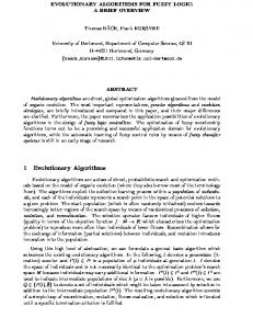
which induces varying variances in fsim over the searchspace. In particular, Eq. (9) is designed such that the standard deviation of fsim(x) varies between 0.5σ and 1.5σ for x ∈ Rn. The parameter γ is to adjust the frequency of this variation, i.e., increasing γ increases the fluctuation rate of the standard deviations between 0.5σ and 1.5σ. Note that γ = 0 induces constant noise with standard deviation σ in fsim. Furthermore, noise at the maximum of fsim is g(0) = σ independent of the choice of γ. In the experiments we denote σ the model noise strength and γ the model noise fluctuation, respectively. Note, that for a model noise strength of σ, the mean absolute deviation of fsim(x) from f(x) is σabs = σ· 2 π . Since the true optimal response is f(0) = 1 we can interpret the noise induced in fsim(0) due to g(0) to be of 100·σabs percent. The two-dimensional response surface of f(x) and variance surface g(x) over the search-space [-1,2]2 are shown in Figures 4 and 5, respectively. We compare the performance of evolution strategies when applying different selection procedures for survivor selection and final selection, respectively (see strategies S1 and S2 in Figure 3). In particular, we compare the combined screening and selection procedure, abbreviated with CSS, the enhanced two-stage selection procedure, abbreviated with ETSS, and the iterative subset selection procedure, abbreviated with ISS, as discussed in Section 3.1. Additionally, we consider the following two simple heuristic selection strategies: MEAN: Perform exactly n0 replicated simulations of each individual and choose the one with the largest mean value. CONF: Perform exactly n0 replicated simulations of each individual and continue replicating until the width of the 100·P* percent t-confidence interval becomes smaller than d*. Then choose the individual with the largest mean value.

-1 -0.5

0 0.5 Factor 1

1

1.5

2 -1

-0.5

0

1 0.5 Factor 2

1.5

2

Figure 5: Variance Surface g(x) for σ = 0.2 and γ = 1.0 In all experiments we apply a (5+5)-ES on the twodimensional sphere function (7) and choose the individuals for the first generation uniformly random in search-space [-1,2]2. For all selection procedures an initial first-stage sample size n0 = 10 and a probability of correct selection P* = 0.9 is used. Furthermore, we assume the indifferencezone parameter d* = 0.1 for the survivor selections and d*/2 for the final selections in order to be more accurate at the end. To introduce unequal variances across the searchspace we choose γ = 1 if not mentioned otherwise. For performance evaluation of the evolution strategy two performance indices are considered: The distance δ between the response of the best solution found by the evolution strategy and the true optimal response, i.e., δ = 1 – f(xopt) where xopt is the result of the evolution strategy, and (ii) the overall number of model evaluations required by the evolution strategy until it returns the result xopt. In order to obtain the performance indices with high confidence we made 10,000 independent replications of the complete optimization process for each point in Figures 6 to 11. In a first experiment the progress of the ES with increasing number of generations is investigated when applying different survivor selection strategies (see Figure 6). In this experiment the model noise strength is σ = 0.2 and the size of the elite population is |B| = 1, i.e., no final selection is used. From Figure 6 we see that for all selection strategies, except the MEAN(10) selection, the distance value approaches 0.01 with increasing number of generations. (i)

847

Buchholz and Thümmler 0.08

Distance from optimal response

require similar number of evaluations but ISS returns a solution with distance 0.011 and MEAN(50) with 0.015, respectively. Comparing the number of evaluations required by the selection strategies we see that the ISS procedure requires the smallest number of evaluations even when producing the best solutions with respect to the distance measure. Recall, that Figure 8 additionally investigates the impact of applying the ISS procedure for final selection. Compared to Figure 7, for all selection strategies the distance measure can be improved about 40% whereas the number of evaluations increases only about 14%. This is a clear argument for using an elite population during the optimization process. In the next experiments we further investigate the impact of applying an elite population. Figures 9 and 10 show the performance indices when increasing the size of the elite population from 1 to 30 for different final selection strategies. For survivor selection we used the MEAN(10) and ISS procedures, respectively. In this experiment the model noise strength is σ = 0.2. For all strategies an increase in elite population size decreases the distance measure and increases the number of evaluations, except for MEAN(10). Observe, that the ETSS procedure does not further improve when the elite population size increases

MEAN(10) MEAN(50) CONF CSS ETSS ISS

0.07 0.06 0.05 0.04 0.03 0.02 0.01 0 0

20

35000

80

100

80

100

MEAN(10) MEAN(50) CONF CSS ETSS ISS

30000 Number of model evaluations

40 60 Number of generations

25000 20000 15000 10000 5000 0 0

20

40

60

Number of generations

Figure 6: Performance Indices for Increasing Number of Generations and Different Survivor Selection Strategies

0.02

Note, that this value is about 10 times smaller than the indifference-zone parameter d*. The reason for this is that the sphere function is very flat, such that the ES produces even after the first generation a result with a distance below 0.1 from the optimal response (see also innermost contour circle around the optimum in Figure 4, which corresponds to a response of 0.9). Considering the number of evaluations required to obtain the results, the selection strategies differ significantly. In fact, the ISS requires about 2/3 of the iterations required by the CSS. In the following experiments we consider a fixed number of 50 generation of the ES until termination. Figures 7 and 8 show the performance indices for σ increasing from 0.01 to 0.3 when applying different survivor selection strategies. In Figure 7 no final selection is considered whereas in Figure 8 the ISS procedure is used for final selection with an elite population of size 10. Comparing the different survivor selection strategies we first observe that distance from the optimal solution increases linearly when applying the MEAN selection strategy. In fact with MEAN selection the accuracy of the solution cannot be controlled automatically with respect to increasing noise. With the other selection strategies the solution accuracy can be significantly increased for all noise levels, but with the cost of a (automatically controlled) larger number of model replications. Furthermore, with the same number of evaluations the ISS procedure produces much better results than the MEAN value approach, e.g. considering a model noise strength of σ = 0.23 in Figure 7, where MEAN(50) and ISS

MEAN(10) MEAN(50) CONF CSS ETSS ISS

Distance from optimal response

0.018 0.016 0.014 0.012 0.01 0.008 0.006 0.004 0.002 0 0

0.05

0.1

0.15

0.2

0.25

0.3

0.25

0.3

Model noise strength 50000

MEAN(10) MEAN(50) CONF CSS ETSS ISS

Number of model evaluations

45000 40000 35000 30000 25000 20000 15000 10000 5000 0 0

0.05

0.1

0.15

0.2

Model noise strength

Figure 7: Performance Indices for Increasing Model Noise Strength, Different Survivor Selection Strategies, and no Final Selection

848

Buchholz and Thümmler 0.02

Distance from optimal response

above 8. The reason for this is that the computation of second-stage sample sizes is based on accurate sample means of the first stage, which are not given for n0 = 10 samples. To tackle this problem, Chen (2002) proposed a conservative adjustment to the ETSS procedure. We also checked this procedure and obtained better results, but, as expected, for a larger number of evaluations. In Figures 9 and 10, the ISS procedure produces almost always the best results with respect to the distance measure; however, it also requires a large number of evaluations. Comparing MEAN(10) and ISS survivor selection, we observe an improvement of about 100% in the distance measure with ISS, whereas the number of evaluations increases only by about 10%. Thus, a conclusion from Figures 9 and 10 is that a simple MEAN selection as usually applied in evolutionary algorithms, should not be the method of choice. In a final experiment in Figure 11, we considered the impact of model noise fluctuation on the performance measures. Again, the model noise strength is σ = 0.2 and the size of the elite population is |B| = 1. From the curves we see how sensitive the selection procedures are against unequal variances across the search-space. Recall, that γ = 0 corresponds to constant variances across the search-space. It can be observed that, procedures CONF, CSS, and ETSS are very stable with respect to the distance measure. Nevertheless, the stability requires an increasing number of evaluations. Considering the MEAN(50) and ISS procedure, we observe an increase in the distance measure for γ between 0 and 1. For the ISS procedure the number of evaluations also increases. This is not desirable, but comparing the absolute numbers ISS produces always the best results with respect to the distance measure as well as the number of evaluations. From the figure we conclude that the performance of ISS as shown in Figures 6 to 10 is further improved when there is small variance fluctuation, i.e., γ < 1. Finally, we state two reasons why selection strategies based on Rinott’s procedure such as CSS require more evaluations than heuristic procedures like ISS or ETSS: (i) the second-stage sample size is based on the variance estimates of the first n0 replications, which might give imprecise estimates resulting in a higher second-stage sample size, and (ii) Rinott’s procedure does not incorporate mean estimates when computing the second-stage sample size, i.e., it assumes the least favorable configuration.

MEAN(10) MEAN(50) CONF CSS ETSS ISS

0.018 0.016 0.014 0.012 0.01 0.008 0.006 0.004 0.002 0 0 50000

0.1 0.15 0.2 Model noise strength

0.25

0.3

0.1 0.15 0.2 Model noise strength

0.25

0.3

MEAN(10) MEAN(50) CONF CSS ETSS ISS

45000

Number of model evaluations

0.05

40000 35000 30000 25000 20000 15000 10000 5000 0 0

0.05

Figure 8: Performance Indices for Increasing Model Noise Strength, Different Survivor Selection Strategies, and ISS Final Selection 0.027

MEAN(10) MEAN(50) CONF CSS ETSS ISS

Distance from optimal response

0.025 0.023 0.021 0.019 0.017 0.015 0.013 0.011 0.009 0.007 0.005 0

5

10

15

20

25

30

Size of elite population 22500

MEAN(10) MEAN(50) CONF CSS ETSS ISS

Number of model evaluations

20000 17500 15000 12500 10000 7500

4.2 Optimization of a Production Line

5000 2500

To provide a more realistic application example, we consider a production line of a manufacturing plant comprising N service queues arranged in a row, that is, parts leaving a queue after service are immediately transferred to the next queue. In this example, we assume all queues to have finite capacity K = 10. Arrivals of parts to the first queue occur according to a Poisson process with rate λ = 0.5.

0 0

5

10

15

20

25

30

Size of elite population

Figure 9: Performance Indices for Increasing Size of Elite Population, Different Final Selection Strategies, and MEAN(10) Survivor Selection

849

Buchholz and Thümmler 0.027

Distance from optimal response

Each queue comprises a single server with first-come, firstserved (FCFS) service discipline and exponentially distributed service time. The service rate (i.e., speed of the server) at queue n is denoted with μn. Furthermore, the vector μ = (μ1,…,μN) of service rates is subject to be optimized by the evolution strategy with respect to a revenue function

MEAN(10) MEAN(50) CONF CSS ETSS ISS

0.025 0.023 0.021 0.019 0.017 0.015 0.013 0.011 0.009

R(μ) =

0.007 0.005 0 22500

10 15 20 Size of elite population

25

30

MEAN(10) MEAN(50) CONF CSS ETSS ISS

20000

Number of model evaluations

5

17500

12500 10000 7500 5000 2500 0 5

10 15 20 Size of elite population

25

30

Figure 10: Performance Indices for Increasing Size of Elite Population, Different Final Selection Strategies, and ISS Survivor Selection 0.014

Distance from optimal response

0.013

0.012

0.011

0.01 MEAN(50) CONF CSS ETSS ISS

0.009

0.008 0

0.5

1

1.5

2

2.5

3

Model noise fluctuation

Number of model evaluations

18000

16000

MEAN(50) CONF CSS ETSS ISS

14000

12000

10000

8000 0

0.5

1

1.5

2

2.5

(10)

where X(μ) is the throughput of the production line (i.e., the time-averaged number of parts leaving the last queue) for service rates μ and r, c0, c1 and c are constants representing a revenue factor, basic costs that occur independent of service rates and a vector with cost factors for each server, respectively. Since X(μ) is decreasing for decreasing any of the μn, n=1,…,N, the revenue function (10) clearly quantifies the trade-off between a high throughput (i.e., a high production rate) and costs of providing fast service. To compute X(μ) quantitative analysis of the model must be conducted. For general models this can only be done by discrete-event simulation. Nevertheless, for the production line model, also numerical transient analysis of the underlying continuous-time Markov chain can be applied for its quantitative solution (Bause, Buchholz, and Kemper 1998). In the experiments, we used the production line with N = 3 queues and considered transient results at time t = 1000 starting with an empty system at time t = 0. The revenue factor and the cost factors are assumed to be r = 10,000, c0 = 1, c1 = 400 and cT = (1,5,9). Furthermore, the searchspace is bounded to μ ∈ [0,2]3, which results in values of R(μ) ranging approximately between –400 and 98.5. Since the optimal solution is unknown we cannot use the distance measure (i) as performance index. Instead we consider the numerical solution Rnum(μopt), where μopt is the result of the evolution strategy. Figure 12 plots the performance indices obtained from 2,500 independent replications of the complete optimization process. In this experiment we considered different survivor selection strategies with d* = 10 and no final selection. It can be observed that ISS produces the best results on average while it requires the smallest number of evaluations. The best solution found during our experiments was Rnum(0.54, 0.45, 0.42) = 98.46. The average revenue of the solutions found by ISS is 94. Considering the range from –400 to 98.5 of possible revenue values this corresponds to 99% of the best solution.

15000

0

r ⋅ X(μ ) − c1 , c0 + cT ⋅ μ

3

Model noise fluctuation

5

Figure 11: Performance Indices for Increasing Noise Fluctuation and Different Survivor Selection Strategies

CONCLUSIONS

In this paper, we presented an evolution strategy for the optimization of simulation models. The proposed evolution strategy determines the parent population of consecutive generations using a statistical selection procedure.

850

Buchholz and Thümmler

REFERENCES

95 94

Arnold, D.V., and H.G. Beyer, A Comparison of Evolution Strategies with Other Direct Search Methods in the Presence of Noise, Computational Optimization and Applications 24, 135-159, 2003. Bause, F., P. Buchholz, and P. Kemper, A Toolbox for Functional and Quantitative Analysis of DEDS, Proc. 10th Int. Conf. on Modelling Tools and Techniques for Computer and Communication System Performance Evaluation, Palma de Mallorca, Spain, Lecture Notes in Computer Science 1469, 356-359, Springer, 1998.

93

Revenue

92 91 90 89 88

MEAN(10) MEAN(50) CONF CSS ETSS ISS

87 86 85 0

25

40000

125

150

MEAN(10) MEAN(50) CONF CSS ETSS ISS

35000

Number of model evaluations

50 75 100 Number of generations

30000



Bechhofer, R.E., T.J. Santner, and D.M. Goldsman, Design and Analysis of Experiments for Statistical Selection, Screening, and Multiple Comparisons, John Wiley & Sons, 1995. Boesel, J., B.L. Nelson, and S.H. Kim, Using Ranking and Selection to “Clean up” After Simulation Optimization, Operations Research 51, 814-825, 2003. Chen, E.J., A Conservative Adjustment to the ETSS Procedure, Proc. Winter Simulation Conference, San Diego, CA, 384-391, 2002. Chen, E.J., and W.D. Kelton, An Enhanced Two-Stage Selection Procedure, Proc. Winter Simulation Conference, Orlando, FL, 727-735, 2000. Chen, E.J., and W.D. Kelton, Inferences From Indifference-Zone Selection Procedures, Proc. Winter Simulation Conference, New Orleans, LA, 456-464, 2003. Fu, M.C., Optimization for Simulation: Theory vs. Practice, INFORMS Journal on Computing 14, 192-215, 2002. Hedlund, H.E., and M. Mollaghasemi, A Genetic Algorithm and an Indifference-zone Ranking and Selection Framework for Simulation Optimization, Proc. Winter Simulation Conference, Arlington, VA, 417-421, 2001. Kemper, P., D. Müller, and A. Thümmler, Combining Response Surface Methodology with Numerical Models for Optimization of Class Based Queueing Systems, Proc. Int. Conf. on Dependable Systems and Networks (DSN), Yokohama, Japan, 2005. Koenig, L.W., and A.M. Law, A Procedure for Selecting a Subset of Size m Containing the l Best of k Independent Normal Populations, With Applications to Simulation, Communications in Statistics – Simulation and Computation 14, 719-734, 1985. Law, A.M., and W.D. Kelton, Simulation Modeling and Analysis, McGraw-Hill, 3rd edition, 2000. Law, A.M., and M.G. McComas, Simulation-Based Optimization, Proc. Winter Simulation Conference, San Diego, CA, 41-44, 2002. Nissen, V., and J. Propach, On the Robustness of Population-Based Versus Point-Based Optimization in the Presence of Noise, IEEE Transactions on Evolutionary Computation 2, 107-119, 1998.

25000 20000 15000 10000 5000 0 0

25

50 75 100 Number of generations

125

150

Figure 12: Performance Indices for Increasing Number of Generations and Different Survivor Selection Strategies Furthermore, we propose to use statistical selection at the end of the evolutionary process for selecting the best individual from a set of candidate best individuals collected during the evolutionary process, i.e., the elite population. As a second contribution we propose a heuristic iterative subset selection (ISS) procedure that reduces a randomsize subset, containing the best individual, to a maximum predefined size. By means of two application examples, we investigated the impact of applying statistical procedures for survivor selections and the final selection. The results show, that the performance of the ES is improved when using statistical selection procedures instead of applying a simple selection based on mean response values. Furthermore, the ISS procedure performs best compared to the other selection strategies for survivor selections as well as the final selection. In future work, we plan to investigate possible improvement of the evolution strategy when using common random numbers (CRN) across systems for the simulation model and compare the performance with selection procedures especially designed for CRN. A second concern is to study the evolution strategy when using a fixed budget allocation, i.e., the maximal number of model evaluations is a predefined value. Finally, we plan to compare the proposed optimization approach with other optimization approaches, especially those based on response surface methodology (Kemper, Müller, and Thümmler 2005).

851

Buchholz and Thümmler

Rinott, Y., On Two-Stage Selection Procedures and Related Probability-Inequalities, Communications in Statistics – Theory and Methods A7, 799-811, 1978. Schwefel, H.P., Evolution and Optimum Seeking, John Wiley, 1995. Sriver, T.A., and J.W. Chrissis, Combined Pattern Search and Ranking and Selection for Simulation Optimization, Proc. Winter Simulation Conference, Washington, DC, 645-653, 2004. Swisher, J.R., S.H. Jacobson, and E. Yücesan, DiscreteEvent Simulation Optimization Using Ranking, Selection, and Multiple Comparison Procedures: A Survey, ACM Transactions on Modeling and Computer Simulation 13, 134-154, 2003.

AUTHOR BIOGRAPHIES PETER BUCHHOLZ is a professor for Modeling and Simulation at the University of Dortmund. Previously he held a professorship at Dresden University of Technology. He holds a diploma, Dr. rer. nat. (Ph.D.) and a habilitation degree, all from the University of Dortmund. His current research interests are analysis techniques for discrete event systems including simulation, the combination of analysis and optimisation and the application of the methods to communication systems and logistic networks. His Web address is . AXEL THÜMMLER is a research scientist in the Modelling and Simulation group at the University of Dortmund. He received the degree Diplom-Informatiker (M.S. in Computer Science) in April 1998 and the degree Dr. rer. nat. (Ph.D. in Computer Science) in July 2003, both from the University of Dortmund. His research interests include simulation optimization, communication networks, mobile computing, and performance evaluation. His Web address is .

852