2D Registration Criterion

Evaluation of a New 3D/2D Registration Criterion for Liver Radio-Frequencies Guided by Augmented Reality St´ephane Nicolau1,2 , Xavier Pennec1 , Luc Soler2 , and Nicholas Ayache1 1

2

INRIA Sophia, Epidaure, 2004 Rte des Lucioles, F-06902 Sophia-Antipolis Cedex {Stephane.Nicolau,Xavier.Pennec,Nicholas.Ayache}@sophia.inria.fr http://www-sop.inria.fr/epidaure/Epidaure-eng.html IRCAD-Hopital Civil, Virtual-surg, 1 Place de l’Hopital, 67091 Strasbourg Cedex {stephane.nicolau,luc.soler}@ircad.u-strasbg.fr

Abstract. Our purpose in this article is to superimpose a 3D model of the liver, its vessels and tumors (reconstructed from CT images) on external video images of the patient for hepatic surgery guidance. The main constraints are the robustness, the accuracy and the computation time. Because of the absence of visible anatomical landmarks and of the “cylindrical” shape of the upper abdomen, we used some radio-opaque fiducials. The classical least-squares method assuming that there is no noise on the 3D point positions, we designed a new Maximum Likelihood approach to account for this existing noise and we show that it generalizes the classical approaches. Experiments on synthetic data provide evidences that our new criterion is up to 20% more accurate and much more robust, while keeping a computation time compatible with realtime at 20 to 40 Hz. Eventually, careful validation experiments on real data show that an accuracy of 2 mm can be achieved within the liver.

1

Introduction

The treatment of liver tumors by radio-frequencies is a new technique which begins to be widely used by surgeons. However, the guidance procedure to reach the tumors with the electrode is still made visually using per-operative 2D crosssections of the patient using either Ultra-Sound (US) or Computed Tomography (CT). Because of the difficulty to locate in 3D the tumor’s center, surgeons estimate that the tumor size has to exceed 2 cm to perform a reliable intervention. Our purpose is to build an augmented reality system that could superimpose reconstructions of the 3D liver and tumor onto a video image in order to improve the surgeon’s accuracy during the guidance step. In such a system, the overall accuracy has to be less than 5 mm to provide a significant help to the surgeon. Just before the intervention, a CT-scan of the patient is acquired and an automatic 3D-reconstructions of his skin, his liver and the tumors is performed [17]. Two cameras (jointly calibrated) are viewing the patient’s skin from two different points of view. The patient is intubated during the intervention, so the N. Ayache and H. Delingette (Eds.): IS4TM 2003, LNCS 2673, pp. 270–283, 2003. c Springer-Verlag Berlin Heidelberg 2003


Evaluation of a New 3D/2D Registration Criterion

271

volume of gas in his lungs can be controlled and monitored. Then, it is possible to fix the volume at the same value during a few seconds repetitively and to perform the CT and the electrode’s manipulation almost in the same volume’s condition. Thus, we assume that a rigid registration is sufficient to register accurately the 3D-model extracted from the CT with the 2D video images. Consequently we are confronted to the classical rigid problem of 3D/3D and 3D/2D Object Registration. Surface and iconic registration using mutual information have been used to register the 3D surface of the face to either video images [18] or another 3D surface acquired with a laser range scanner [5]. In both cases, thanks to several highly curved “edges” on the model (nose, ears, eyes), the reported accuracy was under 5 mm. We believe that in our case, the “cylindrical” shape of the human abdomen is likely to lead to much larger uncertainties along the cranio-caudal axis. Landmarks 3D/3D or 2D/3D registration can be performed when several precisely located points are visible both in the 3D-model and in the video images. Since the landmarks are really homologous, the “cylindrical” geometry of the underlying abdomen surface is not any more a problem. As there are no visible anatomical landmarks in our case, we chose to stick to the patient skin some radio-opaque markers that are currently localized and matched interactively. This problem was largely considered in a wide variety of cases. Closed-form solution for few points [2,1] and linear resolution [3] were proposed in the last decades to find the registration as quickly as possible to fulfill real-time constraints. Others [9,15] determine the object pose by minimizing the classical projective least-squares (LSQ) error function. In these cases, the methods differ by the minimization procedure and by the rotation parameterization. Haralick [6] and Or [10] turn the 2D/3D problem into a 3D/3D points registration problem in which they estimate the depth of the points seen in the image by minimizing a 3D LSQ Euclidean distance criterion. Finally, Yuan and Liu [19,8] solve the problem by separating the rotational components from the translational one. Linear and closed-form solution provide a direct resolution, but they are very sensitive to noise because they assume that data points are exact. As the accuracy is crucial in our application, we cannot afford using them. An alternative approach that separates the rotation from the translation was examined by Kumar [7], and he shows that it leads to worse parameters estimation in the presence of noise than the classical LSQ estimation. Therefore, we think that a LSQ criterion has a definite advantage among the other methods because it can take into account the whole information provided by the data. However, all of the existing methods implicitly consider that 2D points are noisy, but that 3D points are exact. In our case, this assumption is definitely questionable, which lead to the development of a new maximum likelihood (ML) criterion generalizing the standard 3D/2D LSQ criterion. Last but not least, LSQ criterion enables the prediction of the noise influence on the final registration. This would be very useful as it would allow us to detect an inaccurate registration. However, this aspect will be considered in a future work.

272

St´ephane Nicolau et al.

In the sequel, we first recall that the classical 2D/3D registration criterion for points correspondences can be considered as a Maximum Likelihood estimation if the 3D points are exact. Then, modifying the statistical assumptions to account for an existing noise on the 3D point measurements, we derive a new and original criterion that generalizes the classical ML one. Section 3 is devoted to the comparative performance evaluation of both criteria with synthetic data while Section 4 focuses on a careful validation with real data.

2

Maximum Likelihood 2D/3D Registration

Let Mi = [xi , yi , zi ] be the 3D points that represent the exact localization of the (l) (l) radio-opaque fiducials in the CT-scan reference frame and mi (l) = [ui , vi ] be the 2D points that represent its exact position in the images of camera (l). In this article, we assume that correspondences are known. To account for occlusion, we use a binary variable ξil equal to 1 if Mi is observed in camera (l) and 0 otherwise. We denote by T  M the action of the rigid transformation T on the 3D point M and by Pl (1 ≤ l ≤ M ) the camera’s projective functions from 3D to 2D (l) such that mi = P (l) (T  Mi ) (we used in our implementation the calibration algorithm of [20]). In the following sections, Aˆ will represent an estimation of a perfect data A, and A˜ an observed measure. Thus, the 3D points measured by ˜ i , and the measured video 2D points m ˜i . the user will be written M 2.1

Standard Projective Points Correspondences (SPPC) Criterion

˜ i = Mi ) and that the 2D points only Assuming that the 3D points are exact (M 2 are corrupted by an isotropic Gaussian noise ηi of variance σ2D , we have: (l)

m ˜i (l) = mi + ηi = P (l) (T  Mi ) + ηi

with ηi ∼ N (0, σ2D )

The probability of measuring the projection of the 3D point Mi at the location m ˜i (l) in image (l), knowing the transformation parameters θ = {T } is given by: p(m ˜i

(l)

1 | θ) = 2 · exp 2πσ2D




˜i (l) 2  P (l) (T  Mi ) − m − 2 · σ2D 2



Let χ be the data vector regrouping all the measurements, in this case the 2D points m ˜i (l) only. Since the detection of each point is performed independently, M N l the probability of the observed data is p(χ | θ) = l=1 i=1 p(m ˜i (l) | θ)ξi . In this formula, unobserved 2D points (for which ξil = 0) are implicitly taken out of the probability. Now, the Maximum likelihood transformation θˆ maximizes the probability of the observed data, or equivalently, minimizes its negative log:

C2D (T ) =

N M   l=1 i=1

ξil

·

  (l) 2  (l) ˜i  P (T  Mi ) − m 2 · σ2D 2

M N   2 + ξil · log[2πσ2D ] (1) l=1 i=1

Evaluation of a New 3D/2D Registration Criterion

273

Thus, up to a constant factor, this ML estimation boils down to the classical LSQ criterion in the 2D coordinates. Of course, this criterion assumes that there is no noise on the 3D points, or that this noise could be distributed over the 2D measurements. This simple hypothesis makes the criterion very easy to optimize because there are only 6 parameters to estimate and lead to a very low calculations cost. However, from a statistical point of view, distributing the 3D error on 2D measurements leads to correlated noises, which does not agree with the independence assumption used to derive the ML estimation. 2.2

Extended Projective Points Correspondences (EPPC) Criterion

To introduce a more realistic statistical hypothesis on the 3D data, it is thus safer to consider that we are measuring a noisy version of the exact points: ˜ i = Mi + ε i M

with

εi ∼ N (0, σ3D ).

In this case, the exact location Mi of the 3D points is considered as a parameter, just as the transformation T . In statistics, this is called a latent or hidden variable, while it is better known as an auxiliary variable in computer vision. Thus, knowing the parameters θ = {T, M1 , . . . MN }, the probability of measuring respectively a 2D and a 3D point is:   (l) (l) ˜ i | θ) = Gσ ˜ and p(M M ˜i − M p(m ˜ i | θ) = Gσ2D P (l) (T  Mi ) − m i i . 3D One important feature of this statistical modeling is that we can safely assume that all 3D and 2D measurements are independent. Thus, we can write the prob˜ ˜ ability of our observation vector χ = (m ˜ 11 , ..., m ˜ 1N , ..., m ˜M ˜M 1 , ..., m N , M1 , ..., MN ) as the product of the above individual probabilities. The ML estimation of the parameters is still given by the minimization of − log(p(χ|θ)): C(T, M1 , . . . MN ) =

N M  N (l) (l)  ˜ i − M i 2  M ˜ i − m i 2 l m + ξ · + K (2) i 2 · σ3D 2 2 · σ2D 2 i=1 i=1 l=1

where K is a normalization constant depending on σ2D and σ3D . The obvious difference between this criterion and the simple 2D ML is that we now have to solve for the hidden variables (the exact locations Mi ) in addition to the previous rigid transformation parameters. An obvious choice to modify the optimization algorithm is to perform an alternated minimization w.r.t. the two groups of variables. Starting from a transformation initialization T0 , we initialize ˜ i and perform a first minimization on T (this corresponds to the Mi with the M optimizing the simple 2D ML criterion). In a second step, we keep the transformation T fixed and we optimize for the Mi . We then continue to alternatively ˆ i of the exact update the transformation Tˆ (given the lastly estimated values M ˆ i (given the lastly estimated transformation Tˆ). Mi ) and the exact positions M The algorithm is stopped when the distance between the two last estimation of the parameters become negligible. The convergence is insured since we minimize the same positive criterion at each step.

274

2.3

St´ephane Nicolau et al.

Dealing with 3D and 2D Anisotropic Noise

Up to now, we considered isotropic 2D and 3D noises. However, most of the CT-scan acquisition are not isotropic (the slice thickness is often larger than the pixel size within a slice). In that case, the markers 3D localization error will most probably be anisotropic:   2 σ3Dx 0 0 2 0  εi ∼ N (0, Σ3D ) with Σ3D =  0 σ3D y 2 0 0 σ3D z This induces very small changes in our ML formulation: we just have to replace ˜ i −Mi 2 in our criterion (Eq. 2) the first term M2·σ by half of the Mahalanobis 2 3D −1  ˜ ˜ distance (Mi − Mi ) · Σ3D · (Mi − Mi ). The same kind of modifications obviously holds for the second term of the equation in the case of a 2D anisotropic noise. 2.4

Link with Reconstruction and 3D/3D Registration

Let us consider that the exact 3D points are measured in the reference frame of the cameras (instead of the CT frame as previously) and that we are looking for the transformation from the camera world to the CT (instead of the reverse as previously). The 3D/2D ML criterion is then rewritten: N M  N (l)  ˜ i − T ∗ M i 2  M ˜ i − P (l) (Mi ) 2 l m C(T, M1 , . . . MN ) = + ξ · +K. i 2 · σ3D 2 2 · σ2D 2 i=1 i=1 l=1

As explained in the section 2.2, this criterion can be optimized iteratively by successively estimating the 3D coordinates and the transformation T . Moreover, it has to be noticed that the change of variable does not affect the transformation to be found. Now, assuming that we are performing an estimation with a largely overestimated σ3D and a correct estimation of σ2D . Around the optimal transformation Tˆ, we will have N N 1  ˜ 1  ˜  M i − T ∗ M i 2   Mi − Tˆ ∗ Mi 2 = σ ˆ3D  σ3D N i=1 N i=1

Thus, the first term of the criterion is negligible with respect to the second term (since σ2D is assumed to be correctly estimated): optimizing for the exact 3D point positions boils down to the minimization of CRec (M1 , . . . MN ) =

N M  

ξil ·  m ˜ i − P (l) (Mi ) 2 (l)

l=1 i=1

This criterion is in fact one of the more widely used reconstruction criterion. Then, after the determination of the 3D coordinates of the points in the cameras

Evaluation of a New 3D/2D Registration Criterion

275

frame, the next step consists in minimizing the criterion with respect to T . As the second term does not depends on T , this corresponds to the minimization of C3Dreg (T ) =

N 

˜ i − T ∗ M i 2 M

i=1

which is no more than the standard 3D LSQ criterion. As a conclusion, the method consisting in reconstructing the position of 3D points from the cameras and then registering in 3D can be viewed as a limit case of our 3D/2D ML criterion where the noise on 3D points is largely overestimated (with respect to the noise on 2D points). On the other hand, we have already seen that the standard 2D ML criterion for 3D/2D registration is a limit case of our 3D/2D ML criterion where the noise on 3D points is largely underestimated or really very small (still with respect to the noise on 2D points). Thus, we may expect our criterion to perform better than these methods when there is effectively some noise on the 3D points and if we have a good estimation of relative 3D and 2D variances.

3

Performances Evaluation and Criteria Comparison

The goal of this section is to assess on synthetic data the comparative effectiveness of the SPPC and EPPC criteria in terms of computing cost, accuracy and robustness. Experiments are realized with two synthetic cameras with a default angle of 45 degrees and jointly calibrated in the same reference frame. The two cameras are focusing on the same 15 points Mi representing the markers localizations, distributed in a volume of about 10 × 10 × 10 cm3 . The ratio of the distance cameras/points with the cameras focal length is 25. We modeled the fiducial localization error by a Gaussian noise with different standard deviations on both the 3D and 2D data (default values are σ3D = σ2D = 2 which corresponds to a SNR of 75 dB1 . The optimization procedure used is the Powell algorithm. The registration error is evaluated using 9 control points Ci different from the Mi to assess a Target Registration Error (TRE) instead of a Fiducial Localization Error (FLE) that does not reflect correctly the real accuracy. For each experiment, we give the mean computation time, the mean RMS TRE and the mean relative error (T RESP P C /T REEP P C ) over 10000 registrations (a value above one means that EPPC is more accurate than SPPC). 3.1

Accuracy Performances

Focusing on the accuracy and not on the robustness, we kept the initial and sought transformation fixed and close enough so that both algorithms do converge correctly. The two following tables present the performances w.r.t. a varying 3D/2D noise ratio (mean TRE values are meaningless and then not reported 1

SN RdB = 10 log10 ( σσns ) where σs (resp. σn ) is the variance of the signal (resp. noise).

276

St´ephane Nicolau et al.

since the noises do vary) and a varying angle between the cameras. In these tables, we should only consider the relative values of the computation times as the absolute value depends on the initialization. Noise ratio σ3D /σ2D 4 2 1 0.5 0.25 Computation SPPC 0.0024 0.0023 0.0024 0.0023 0.0024 time (sec.) EPPC 0.119 0.057 0.025 0.024 0.021 Mean relative error 1.17 1.15 1.09 1.03 1.006 Cameras angle Computation SPPC time (sec.) EPPC Mean TRE SPPC (mm) EPPC Mean relative error

90 60 45 30 10 0.0025 0.0034 0.0026 0.0025 0.0031 0.015 0.021 0.025 0.028 0.022 1.76 1.94 2.14 2.50 4.12 1.75 1.83 1.94 2.22 3.40 1.008 1.051 1.089 1.114 1.188

One can see that EPPC always provides a better TRE (up to 20%) than SPPC, at the cost of a 10 to 20 times larger computational time. The gain in accuracy is all the more sensitive that the angle between the cameras is small and the 3D noise is important w.r.t. the 2D noise. As the amount of 3D information depends on these two parameters, this results was expected since EPPC better captures than the SPPC the noisy nature of information on 3D data. Eventually, the following table presents the influence of the number of points on the computation times and accuracy performances. Number of points 30 15 8 4 Computation SPPC 0.0042s 0.0026s 0.0016s 0.0011s time (sec.) EPPC 0.067s 0.025s 0.011s 0.006s Mean TRE SPPC 1.55 2.16 2.73 4.45 (mm) EPPC 1.42 1.97 2.51 3.94 Mean relative error 1.080 1.090 1.079 1.117 The first observation is that the computation times are roughly proportional to the number of points. This was foreseeable since the computational complexity is linear in the number of data points. The second observation is that the measured TRE seems inversely proportional to the square root of the number of points (multiplying 2 times the number of points decrease the RMS error by a factor √ 2). This is also in accordance with the standard accuracy improvements in statistics. One interesting consequence is that we need about 15% less points with EPPC than with SPPC to reach the same accuracy on this example. 3.2

Robustness Evaluation

To evaluate the robustness w.r.t the initial transformation, we select a random initial and/or sought transformation (uniform rotation and translation in a range of the order of the cameras’ field of view), random 2D (resp. 3D) noises from 1 to 3 pixels (resp. mm), and a random angle between the cameras (from 10

Evaluation of a New 3D/2D Registration Criterion

277

to 90 degrees). In the following table, we display the performance results when the transformation is initialized using the identity or randomly. The first case represents the usual situation where we have no prior information, and the second one simulates a very bad initialization.

Computation SPPC time EPPC Ratio of wrong SPPC convergence (RWC) EPPC Mean relative error

Random T with Random T with identity initialization random initialization 0.0223s 0.0250s 0.138s 0.342s 20.07% 31.55% 0.09% 0.67% 1.107 1.139

In both cases, one can see that the SPPC converges wrongly in broadly 20% of the case, whereas the EPPC almost always converges toward the optimal transformation (RWC under 1%). The difference in performances between the two columns probably comes from the optimization algorithm (Powell) that uses a research domain centered around the identity. Another optimization scheme may lead to slightly different results. 3.3

Computation Times

EPPC is a more accurate and much more robust criterion than SPPC. This is paid by a higher computation time that remains however limited to a few tenths of seconds when the initialization is unknown, and to 0.025 to 0.05 seconds when the initialization is close to the sought transformation. Thus, in view of a realtime system, one may expect to obtain with EPPC the best performances with an initialization time of say 0.3 sec. and an update rate of 20 to 40 Hz if the motions are sufficiently slow w.r.t. the video-rate. One may further improve the tracking rate by updated the “exact 3D coordinates” only once in a while or using a Kalman filter.

4

Performances Assessment with Real Data

This section is devoted to accuracy experiments with real 3D CT-scans and 2D images of a plastic mannequin with approximately 25 fiducials sticked on its surface. Ideally, the method’s accuracy should be assessed by comparing each registration result with a gold-standard that relates both the CT and the camera coordinate systems to the same physical space, using an external and highly accurate apparatus. As such a system is not available (otherwise we would not have to develop a 3D/2D registration algorithm), we adapted the registration loops protocol introduced in [13,16,14], that enables to measure the TRE error for a given set of test points. The principle is to acquire several CT scans of the mannequin that are registered using a method described below. Then, several couples of 2D images are

278

St´ephane Nicolau et al. CT1

CT2

Bronze Standard T CT1/CT2

3D Points extraction with noise

3D Points extraction with noise

3D set1:

3D set2:

x1 y1 z1 x2 y2 z2

x1 y1 z1 x2 y2 z2

. . xt yt zt

. . xp yp zp

Consistency measure 3D/2D registration T CAM1/CT1

3D/2D registration T CAM2/CT2

2D set1:

2D set2:

2D set3:

2D set4:

u1 v1 u2 v2 . . . ui vi

u1 v1 u2 v2 . . . uj vj

u1 v1 u2 v2 . . . uk vk

u1 v1 u2 v2 . . . ul vl

2D Points extraction with noise

IMAGE 1

IMAGE 2 CAM 1

2D Points extraction with noise

IMAGE 1

IMAGE 2 CAM 2

The cameras are calibrated together in the same world coordinate

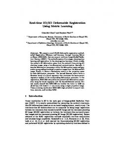
Fig. 1. Registration loops used to estimated the registration consistency.

acquired with the cameras jointly calibrated so that we can compare independent 3D/2D registration of the same object (different 2D and 3D images). A typical loop is sketched in Fig. 1: a test point in the faked liver of CT1 is transformed into the CAM1 coordinate system using a first 3D/2D registration, then into the coordinate system of CT2 using a second 3D/2D registration (the coordinate system of CAM1 and CAM2 are identical since cameras are jointly calibrated), and back to CT1 using the bronze standard registration. Using two different CT im-

Evaluation of a New 3D/2D Registration Criterion

279

ages allows to de-correlate the two 3D/2D transformation. Indeed, if we register the 2D points to the same set of 3D points (extracted from a single CT scan), the two transformations are similarly affected by the 3D points errors. Consequently, the variability of the 3D points extraction (and any possible bias) is hidden. If all transformations were exact, we would obtain the same position for our test point. Of course, since the transformations are not perfect, we measure a Target Registration Error (TRE) whose variance is σ 2 loop = 2σ 2 CAM/CT + σ 2 CT /CT . This experiment providing only one error measurement, we still need to repeat it with different datasets to obtain statistically significant measures. In order to take into account possible calibration error and/or bias, it is necessary to repeat the experiment with different calibrations and positions of the cameras, and not only to move the object in the physical space. As a result, we are able to measure σ 2 loop and thus to estimate the variability due to the 3D/2D registration σ 2 CAM/CT , provided we know σ 2 CT /CT . For this purpose, we devise the following experimental procedure based on multiple CT scan registration that not only gives a very accuracy registration between CT images, but also evaluates the accuracy of this registration. 4.1

Bronze Standard Registration between the CT Images

Our goal here is to compute the n − 1 most reliable transformations T¯i,i+1 that relate the n (successive) CTi images. Estimations of these transformations are readily available by computing all the possible registrations Ti,j between the CT images using m different methods ([16]). Then, the transformations T¯i,i+1 that best explain these measurements are computed by minimizing the sum of the squared distance between the observed transformations Ti,j and the corresponding combination of the sought transformation T¯i,i+1 ◦ T¯i+1,i+2 . . . T¯j−1,j . The distance between transformations is chosen as a robust variant of the left invariant distance on rigid transformation developed in [13]. The estimation T¯i,i+1 of the perfect registration Ti,i+1 is called bronze standard because the result converges toward Ti,i+1 as m and n become larger. Indeed, considering a given registration method, the variability due to the noise in the data decreases as the number of images n increases, and the registration computed converges toward the perfect registration up to the intrinsic bias (if there is any) introduced by the method. Now, using different registration procedures based on different methods, the intrinsic bias of each method also becomes a random variable, which is hopefully centered around zero and averaged out in the minimization procedure. The different bias of the methods are now integrated into the transformation variability. To fully reach this goal, it is important to use as many independent registration methods as possible. In our setup, we used five CT scan of the plastic mannequin in different positions, and five different methods with different geometric features or intensity measures. Three of these methods are intensity-based: the algorithm aladin [11] has a block matching strategy where matches are determined using the coefficient of correlation, and the transformation is robustly estimated using a leasttrimmed-squares; the algorithm yasmina uses the Powell algorithm to optimize

280

St´ephane Nicolau et al.

the SSD or a robust variant of the correlation ratio (CR) metrics between the images [16]. For the feature-based methods, we used the crest lines registration described in [12], and the multi-scale EM-ICP algorithm of [4] on zero-crossings of the Laplacian surfaces (the images were down-sampled by a factor of 2 to limit the number of surface points to about 1.5 million...). Since none of these methods uses the 3D extracted points as registration data, we ensure the independence with respect to the marker localization noise that corrupts the 3D/2D registration. As a side effect, we may use only four of the five methods to determine the bronze standard registration, and use that standard to determine the accuracy of the fifth method (a kind of leave-one-method-out test). This uncertainty is then propagated into the final bronze standard registration (including all methods) to estimate its accuracy. In the table below, we give the standard deviation determined this way on the rotational and translational components of each method, the uncertainty of the resulting bronze standard registration and the uncertainty of the 3D registration using standard least-squares of the fiducial markers positions (w.r.t. the bronze standard). σrot (deg) σtrans (mm) Aladin 0.09 0.56 Yasmina SSD 0.02 0.41 Yasmina CR 0.06 0.41 Crest lines 0.04 0.27 EM-ICP 0.08 0.68 Bronze standard 0.01 0.07 Fiducials 0.15 0.85 One can observe that the crest lines registration is performing the best, quickly followed by the Yasmina registrations. EM-ICP is not performing very well due to the down sampling of the images. The final bronze standard registration accuracy is very good (it corresponds to 0.08 mm TRE on the test points). Finally, we point out that the lack of accuracy of the fiducials registration w.r.t. the other methods is due to the fact that the markers were stick on the “skin” of the mannequin, which is elastic and did move by about 1 to 2 mm between the acquisitions, while all other methods did focus on the rigid structure of the mannequin (this effect was checked on the images after registration). 4.2

Validation Results and Discussion

After the bronze standard registration of our 5 CT images of the mannequin, we took pictures of the mannequin in four different positions with four different cameras and three different (but joint) calibrations. As a result, we have 12 pairs of 2D images to register to 5 CT scans for each pair of cameras (the second pair of camera being used to close the registration loop on a different CT scan). To robustify the experiment, we randomized the camera used in each pair among the four available, which finally leads to 180 registration loops. Approximately

Evaluation of a New 3D/2D Registration Criterion

281

25 stick fiducials were interactively localized in each image (σ3D = 0.75 mm, σ2D = 2.0 pixel). This lead to the following quantitative evaluation. Angle between the cameras 60o 40o 10o Computations SPPC 0.023 s 0.025 s 0.027 s time EPPC 0.21 s 0.21 s 0.25 s Mean TRE RMS SPPC 1.80 1.99 2.30 error in mm EPPC 1.70 1.83 2.20 Relative error 1.062 1.089 1.054 One can observe that EPPC is always more accurate than SPPC but the relative error does not increase as much as denoted with synthetic data when the angle is small (10o ). This may be explained by the various conditions in which the measurement were done (different local lengths, number of fiducial observed...), and the simple representation of the camera (pinhole model). Another explanation is obviously the consistent but non-rigid motion (mentioned in the last section) of the skin markers on which the registration is done. However, these small movements realistically simulate the imperfect repositioning of the skin and the organs that is induced by our gas volume monitoring protocol. In this context, the assumption (on which are based our criteria) of independent noises on each 3D marker position may not be fulfilled. Despite these variations from the theoretical assumptions, we underline that the achieved accuracy is around 2mm, which is by far better than the 5mm needed for our medical application. One can assess the visual accuracy of our registration on one particular case in Fig. 2.

5

Conclusion

We devised in this paper a new 2D/3D Maximum Likelihood registration criterion (EPPC) based on better statistical hypotheses than the classical 3D/2D least-square registration criterion (SPPC). Experiments on synthetic and real data showed that EPPC is 5 to 20% more accurate and much more robust than SPPC, but requires higher computation times when the initialization is unknown (0.3 instead of 0.03 sec.). However, synthetic experiments provide evidences that a refreshment rate of 20 to 40 Hz is achievable in a tracking phase, where only small motions have to be detected. In the context of augmented reality for liver radio-frequencies, we showed that the proposed method provides an accuracy of about 2mm within the liver, which fits the initial goal of 5mm that was necessary to provide a significant help for radiologists and surgeons. In the future, we will focus on the automatic detection, tracking and matching of the fiducials in the 3D and 2D images, in order to fully automate the algorithm. Incidentally, we expect to obtain a much better (probably sub-pixel) localization of the fiducials, and thus drastically improve the accuracy of the 3D/2D registration down to less than one millimeter. We will also investigate the effects of the optimization procedure and of the camera calibration algorithm. Another work in progress concerns the prediction of the uncertainty of

282

St´ephane Nicolau et al.

Fig. 2. The top left image shows the plastic mannequin with the radio-opaque fiducials. The top right image displays the augmented reality view of the surgeon, i.e. the superimposition on the video image of the 3D reconstruction of the fiducials and interns parts (plastic frame and liver) after the registration process. To check visually the quality of the achieved registration on the liver, we put off the skin (bottom left image), and we superimposed the reconstruction of the fiducials on the liver (bottom right).

the 3D/2D registration w.r.t. the current data used. This important element of the system safety will allow the detection of bad geometric fiducials configurations (for instance not enough fiducials visible in both cameras, etc) that lead to very inaccurate registrations. Lastly, we intend to extend the current system in order to take into account the deformations due to breathing.

References 1. M. Dhome and al. Determination of the attitude of 3d objects from a single perspective view. IEEE Trans. on PAMI, 11(12):1265–1278, December 1989. 2. M. Fischler and R. Bolles. Random sample consensus : A paradigm for model fitting with applications to image analysis and automated cartography. Com. of the ACM, 24(6):381–395, June 1981. 3. S. Ganapathy. Decomposition of transformation matrices for robot vision. Pattern Recognition Letters, 2(6):401–412, December 1984.

Evaluation of a New 3D/2D Registration Criterion

283

4. S´ebastien Granger and Xavier Pennec. Multi-scale EM-ICP: A fast and robust approach for surface registration. In A. Heyden, G. Sparr, M. Nielsen, and P. Johansen, editors, European Conference on Computer Vision (ECCV 2002), volume 2353 of LNCS, pages 418–432, Copenhagen, Denmark, 2002. Springer. 5. W. Grimson and al. An automatic registration method for frameless stereotaxy, image-guided surgery and enhanced reality visualization. IEEE TMI, 15(2):129– 140, April 1996. 6. R. Haralick and al. Pose estimation from corresponding point data. IEEE Trans. on Systems, Man. and Cybernetics, 19(06):1426–1446, December 1989. 7. R. Kumar. Determination of camera location and orientation. In DARPA Image Understanding Workshop, pages 870–881, Palo Alto, Calif., 1989. 8. Y. Liu and al. Determination of camera location from 2d to 3d line and point correspondences. IEEE Trans. on PAMI, 12(01):28–37, January 1990. 9. D. Lowe. Fitting parameterized three-dimensional models to images. IEEE Trans. on PAMI, 13(5):441–450, May 1991. 10. Siu-Hang Or and al. An efficient iterative pose estimation algorithm. In Proc. of ACCV’98, pages 559–566, 1998. 11. S. Ourselin, A. Roche, S. Prima, and N. Ayache. Block Matching: A General Framework to Improve Robustness of Rigid Registration of Medical Images. In Proc. of MICCAI’00, pages 557–566, Pittsburgh, Penn. USA, October 11-14 2000. 12. X. Pennec, N. Ayache, and J.-P. Thirion. Landmark-based registration using features identified through differential geometry. In I. Bankman, editor, Handbook of Medical Imaging, chapter 31, pages 499–513. Academic Press, September 2000. 13. X. Pennec, C.R.G. Guttmann, and J.-P. Thirion. Feature-based registration of medical images: Estimation and validation of the pose accuracy. In MICCAI’98, LNCS 1496, pages 1107–1114, October 1998. 14. G. Penney and al. Overview of an ultrasound to ct or mr registration system for use in thermal ablation of liver metastases. In MIUA’01, July 2001. 15. T. Phong and al. Object pose from 2-d to 3-d points and line correspondences. IJCV, 15:225–243, 1995. 16. A. Roche, X. Pennec, G. Malandain, and N. Ayache. Rigid registration of 3D ultrasound with MR images: a new approach combining intensity and gradient information. IEEE TMI, 20(10):1038–1049, October 2001. 17. L. Soler and al. Fully automatic anatomical, pathological, and functional segmentation from ct-scans for hepatic surgery. Computer Aided Surgery, 6(3), August 2001. 18. P. Viola and W.M. Wells. Alignment by maximization of mutual information. International Journal of Computer Vision, 24(2):137–154, 1997. 19. J. Yuan. A general photogrammetric method for determining object position and orientation. IEEE Trans. on Robotics and Automation, 5(2):129–142, April 1989. 20. Zhengyou Zhang. A flexible new technique for camera calibration. Technical report, Microsoft Research, December 1998.